| Computer Modeling in Engineering & Sciences |
DOI: 10.32604/cmes.2022.020111
ARTICLE
Topology Optimization of Self-Supporting Structures for Additive Manufacturing with Adaptive Explicit Continuous Constraint
College of Safety Science and Engineering, Civil Aviation University of China, Tianjin, 300300, China
*Corresponding Author: Jun Zou. Email: sc.zoujun@gmail.com
Received: 04 November 2021; Accepted: 29 December 2021
Abstract: The integration of topology optimization (TO) and additive manufacturing (AM) technologies can create significant synergy benefits, while the lack of AM-friendly TO algorithms is a serious bottleneck for the application of TO in AM. In this paper, a TO method is proposed to design self-supporting structures with an explicit continuous self-supporting constraint, which can be adaptively activated and tightened during the optimization procedure. The TO procedure is suitable for various critical overhang angles (COA), which is integrated with build direction assignment to reduce performance loss. Besides, a triangular directional self-supporting constraint sensitivity filter is devised to promote the downward evolution of structures and maintain stability. Two numerical examples are presented; all the test cases have successfully converged and the optimized solutions demonstrate good manufacturability. In the meanwhile, a fully self-supporting design can be obtained with a slight cost in performance through combination with build direction assignment.
Keywords: Topology optimization; additive manufacturing; self-supporting constraint; build direction assignment; gradual evolution
Additive manufacturing (AM) is a free-form manufacturing technique that builds parts in layers by depositing fine powder material, which is advantageous in building parts with complex shapes without specific tooling or fixturing [1]. However, the AM is not an economical technology for conventional design, and the advantages can only be brought into play adequately through the elaborate design of high-performance structures. Topology optimization (TO) is an advanced structural design method that can be adopted to find the optimal material distribution within a given design domain under certain constraints. The state-of-the-art TO methods include homogenization method [2], solid isotropic material with penalization (SIMP) [3,4], evolutionary structural optimization (ESO) [5], level set method [6], moving morphable components (MMC) [7] and moving morphable void (MMV) [8]. The integration of TO and AM technologies shows the potential to create significant synergy benefits [1].
In general, the results produced by conventional TO methods may not be built directly via AM. There are some manufacturing limitations that should be catered, such as minimum feature size, minimum slot distance, overhang limitation, material anisotropy, and microstructure control [1,9]. The lack of AM-friendly TO algorithms is a serious bottleneck for the application of TO in AM [10]. Liu et al. [1] and Zhu et al. [11] summarized the state-of-art researches conducted on the integration of TO and AM for a variety of topics in recent years.
Overhang constraint is one of the most troublesome manufacturing limitations that are inherent within AM. When the overhang portions of a structure have inclination angles smaller than the critical overhang angle (COA), auxiliary supports are required to provide mechanical support and/or promote heat dissipation, otherwise the part will collapse during the AM process. Thomas [12] identified 45° as the COA for the parts manufactured with 316L stainless steel powder using SLM, while Wang et al. [13] found out that the overhang surfaces can always be well-printed if the overhang angles exceed 34°. Leary et al. [14] adopted 40° as the COA for those parts manufactured by fused deposition modelling (FDM). The auxiliary supports need to be removed after manufacturing, which will extend the build time, and increase material cost. The ideal approach is to integrate the COA restriction in the TO process, so that the solutions are self-supported and eliminates the need for additional supports.
Within the SIMP framework, Serphos [9] integrated the geometrical restriction in the optimization process through three strategies: multiple objective functions, global explicit constraint and density filter. Gaynor et al. [15,16] presented a support region projection to ensure a feature that is adequately supported, Then, Johnson et al. [17] made some improvements to allow for specifying COAs through an updated support region. Langelaar [18,19] introduced a self-supporting filter to rigorously exclude the geometries that violate the overhang angle criteria. Zhao et al. [20] devised an explicit quadratic continuous constraint to represent the self-supporting requirement. Qian [21] developed a Heaviside projection integral form with explicit geometric meanings based on the density gradient. Then, Wang et al. [22] introduced an approach that can be taken to optimize the build direction and topological layout simultaneously. van de Ven et al. [23,24] introduced an overhang filter with which the overhang regions can be detected by an anisotropic speed function. Garaigordobil et al. [25] proposed an overhang constraint based on an edge detection algorithm developed in the field of image analysis and processing. Zhang et al. [26] developed a method that can be applied to estimate the structural boundary normal by fitting local element density distribution with linear surfaces. Luo et al. [27] controlled the minimal overhang angle only in the enclosed voids to reduce the performance loss, and the inward-pointing normal is evaluated by the density gradient.
In addition to the SIMP frameworks, Mirzendehdel et al. [28] put forward a topological sensitivity approach for constraining support structure volume with in the level set framework. Liu et al. [29] proposed a multi-level set interpolation to address the support-free manufacturability constraint. By adopting polygon-featured holes as the basic design primitives, Zhang et al. [30] introduced the overhang constraints directly into the geometry description. Wang et al. [31] proposed a new form of overhang constraint in the level set framework, which is expressed as a single domain integral instead of point-wise constraints. Based on the MMC and MMV frameworks, Guo et al. [32] addressed the overhang limitation by constraining the angle of the curve boundaries. Zhao et al. [33] proposed a density filter within homogenization theory-based method to ensure that the porous structure satisfies the self-supporting constraint. Wang et al. [34] presented a B-spline based method to design self-supporting structures, in which an overhang angle constraint and a triangle constraint are presented.
This article presents an extension and improvement of the work presented in Zou et al. [35], in which an explicit self-supporting constraint model is constructed. The non-trivial improvements made in this article are as follows. Firstly, the improved method is applicable to various values of COA other than 45°. Secondly, the TO optimization process is combined with build direction assignment to reduce the performance loss. Thirdly, an adaptive explicit continuous constraint is devised to control the stability of structural evolution. Lastly, a triangular directional self-supporting constraint sensitivity filter is proposed to promote the downward evolution of structures and maintain stability. Furthermore, the volume preserving Heaviside projection filter [36] is adopted to suppress the gray elements and ensure the stability of optimization.
The remainder of this article is organized as follows. Section 2 introduces the formulation of the adaptive explicit self-supporting constraint in the SIMP framework. Section 3 introduces the problem formulation and TO procedure combined with build direction assignment. In Section 4, two numerical examples are presented to demonstrate the effectiveness of the proposed method. The conclusions are drawn in Section 5.
2 Self-Supporting Constraint Formulation in SIMP Framework
2.1 Brief Introduction of SIMP
The SIMP method is a widely used TO method, in which the elements of the discretized design space are assigned with continuous variables such as material density. The material properties such as Young's modulus are a function of the element density given by the interpolation scheme. In general, a penalization factor is introduced by raising the density to the power of this penalization factor to ensure black-and-white solutions. Besides, filtering methods should be applied to avoid checkerboards and mesh-dependency solutions. Compliance minimization is one of the most common TO problems applied for weight saving in various industries, which can be formulated as Eq. (1):
where c represents the compliance, F indicates the force vector and U denotes the nodal displacement vector.
A SIMP interpolation scheme proposed in Sigmund [37] is introduced to ensure black-and-white solutions, as formulated in Eq. (2):
where E0 is the Young's modulus after the interpolation. Emin is the stiffness of void material to void singularity of the stiffness matrix, which is generally considered as Emin = 10−9. p denotes the penalization factor, which is taken as 3 generally.
2.2 Adaptive Self-Supporting Constraint Formulation
The continuous characteristics of the design domain, such as element density gradient, can be relied on to identify the structural boundary and inclined angles, while this additional step is expected to make the optimization problem overly complex. In this article, the discrete element density is adopted to identify the unsupported elements. This article only considers the 2D rectangular region problems, in which all four sides of the design domain can be considered as the potential baseplate. They are denoted respectively as B, R, U, and L, as shown in Fig. 1. In order to adapt to various COAs, the design domain is discretized into rectangular elements, in which the element aspect ratio b/a is made adjustable according to the magnitude of COA and build direction. Take the bottom side as an example. Each solid element should be sufficiently supported by the three adjacent elements in the underlying layer.
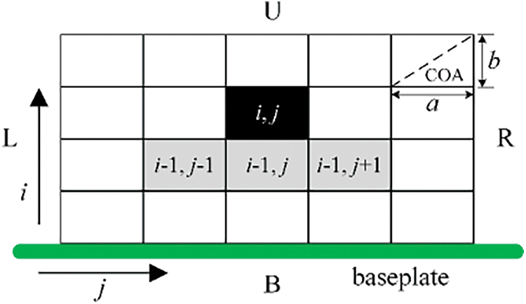
Figure 1: Definition of supporting regions
The mathematical model of self-supporting criterion is defined as:
where
Eq. (3) can be used to judge the supporting status of each elements, and then an explicit constraint function
where parameter
For a clear black-and-white topology, it can be seen clearly that
Different from the compliance, the self-supporting constraint is a local feature. In the early optimization iterations, there exist a large number of intermediate elements, and the structural boundary is blurry. In this circumstance, the constraint evaluation is inaccurate and meaningless. In order to make the optimization process more stable and prevent the local optimal solution with poor performance, a reasonable idea is to make the upper bound of constraint assigned and tightened adaptively during the optimization process. Therefore, the value of ɛ is large enough first to keep the self-supporting constraint inactivated until the structural compliance becomes stable. Then, the constraint is activated artificially and the following scheme is used for ɛ to decrease from
where loop0 and
3.1 Topology Optimization Formulation Combined with Build Direction Assignment
The formulation of minimum compliance structural topology optimization subject to volume constraint and self-supporting constraint is demonstrated in Eq. (7), which is combined with build direction assignment to reduce performance loss. The structural compliance, volume constraint and self-supporting constraint are evaluated based on the physical density
where variable d is the build direction. For simplicity, only the 4 build directions, denoted as B, R, U, and L in Fig. 1, are taken into consideration. Nevertheless, test results show that the performance loss can be reduced in a large extent.
To avoid the formation of checkerboard patterns, intermediate field of densities
where Hei is the weight factor, Ne is the set of elements i for which the center-to-center distance (e, i) to element e is smaller than the filter radius R1.
Since the linear filter averages the density distribution and is not good to obtain an ideal black-and-white design, the volume preserving Heaviside projection filter proposed by Xu et al. [36] is applied after the linear filter in Eq. (8) to obtain the physical density
where β is a parameter controls the smoothness of the approximation. The Heaviside function has such a property: if 0 ≤
In addition, it should be noted that the self-supporting constraint
3.2 Sensitivity Analysis and Triangular Directional Sensitivity Filter
The optimization problem is solved by the gradient based algorithm Method of Moving Asymptotes (MMA) proposed by Svanberg [38]. As for the sensitivity analysis of objective function c and volume constraint V, reference can be made to Andreassen et al. [39]. The sensitivities of self-supporting constraint
The sensitivity analysis ignores the knock-on effect of unsupported elements, for which the change in
As for the second and third terms on the right side of Eq. (10), reference can be made to Xu et al. [36] and Andreassen et al. [39], respectively. It can be easily found out that the sensitivity values are nonpositive, which means that the constraint value is reduced by increasing the element densities below the unsupported elements, and self-supporting is realized by gradual downward evolution of structural boundaries.
In order to promote the downward evolution of structural boundaries and avoid tiny supporting structures, a directional self-supporting sensitivity filter is proposed in this article. Used in the previous works, a semicircular directional sensitivity filter will inherently lead to some unsupported elements at the bottom of semicircle, and cause disturbance to some degree. In this article, a triangular directional self-supporting constraint sensitivity filter is devised as follows:
where Ne is the set of elements within the triangular as shown in Fig. 2a. Hei is a weight factor. The unit of R2 and distance (e, i) is the number of elements, so that the actual shape of the triangle varies according to the element aspect ratio. As the example illustrated in Fig. 2b, the solid element is unsupported. Through the action of the proposed directional sensitivity filter, the modified sensitivities are all negative in the upside down triangle area, which promotes the downward evolution and avoids tiny supporting structures.
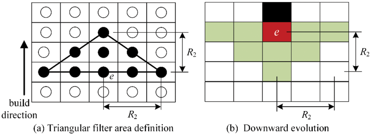
Figure 2: The illustration of the triangular directional self-supporting sensitivity filter
3.3 Topology Optimization Procedure
A flowchart of the TO optimization procedure with self-supporting constraint that is combined with build direction assignment is demonstrated in Fig. 3. Firstly, the value of ɛ is large enough to keep the self-supporting constraint inactivated, which means that the design space is optimized for minimum compliance in the early stage of optimization. If the change rate of compliance less than 0.01, the constraint values are evaluated in different build orientations as described in Section 3.1, and assign the build direction to the orientation that owns the minimum self-supporting constraint value. Then, the design domain is remeshed if necessary, and the element densities are reassigned by means of interpolation in line with the current design, and the self-supporting constraint is activated as described in Eq. (6). If the change rate of both compliance c and
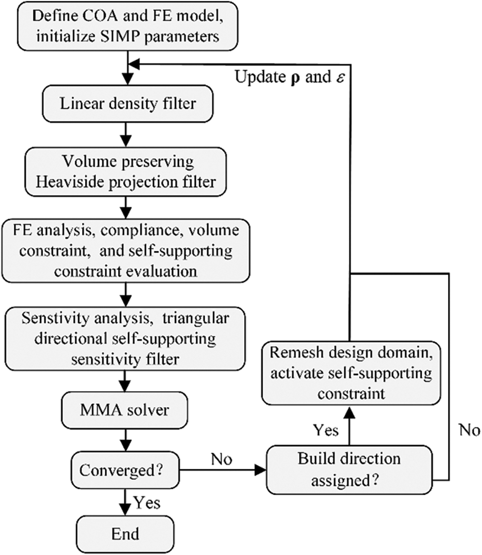
Figure 3: Flowchart of the topology optimization procedure
Two numerical examples are discussed in this chapter to demonstrate the effectiveness of the developed optimization process. The material is isotropic with Young's modulus E0 = 1 and Poisson's ratio ν = 0.3. The self-supporting constraint parameters are set as k = 150,
The problem statements and boundary conditions of the MBB beam problem are illustrated in Fig. 4. The design domain is a rectangular area with a width of 150 and height of 50. A unit load is applied on the middle point of the top of the design domain. The initial value of Heaviside projection parameter β is set to 1 and doubled every 50 iterations.
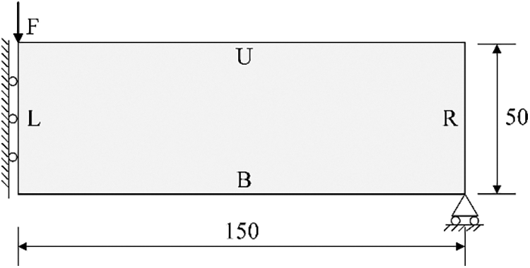
Figure 4: The design domain of MBB beam example
For comparison, the MBB problem is first optimized without the self-supporting constraint. The volume restriction is taken to be 40% of the domain, and density filter is applied with a radius of 3.5. The optimal free design is depicted in Fig. 5 with compliance cref = 229.20, which is treated as a reference for the results with self-supporting constraint. It is easy to find out that the dome and bottom of the structures are totally horizontal, which cannot be manufactured in vertical direction. As a result of Heaviside projection, the transition zone becomes very narrow and leads to a clear structural configuration.
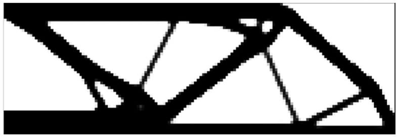
Figure 5: Optimum design for the MBB beam without self-supporting constraint, cref = 229.20
When the self-supporting constraint is considering, the COA is first set to 45°, while parameter
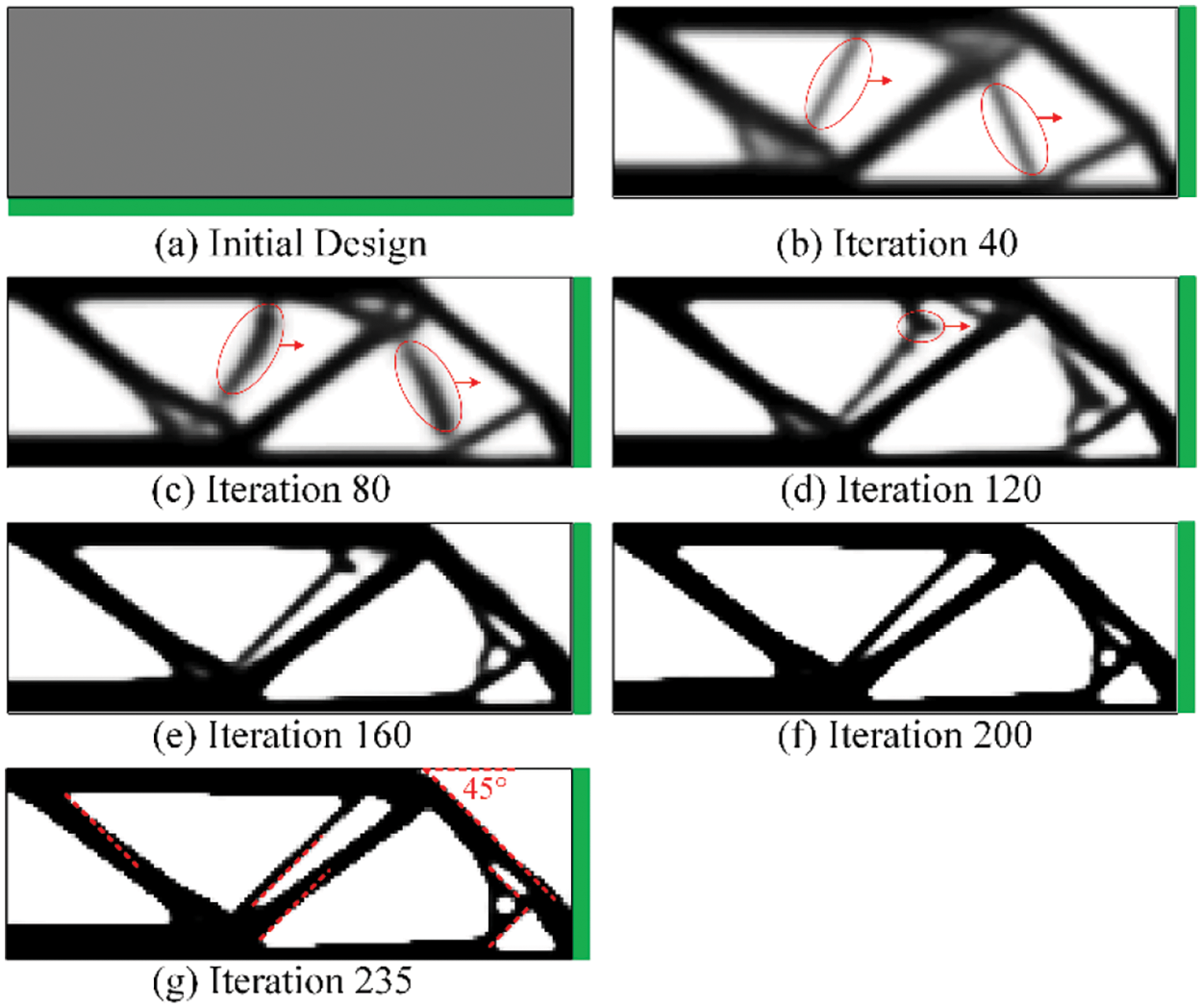
Figure 6: Design evolution history of the MBB beam with self-supporting constraint
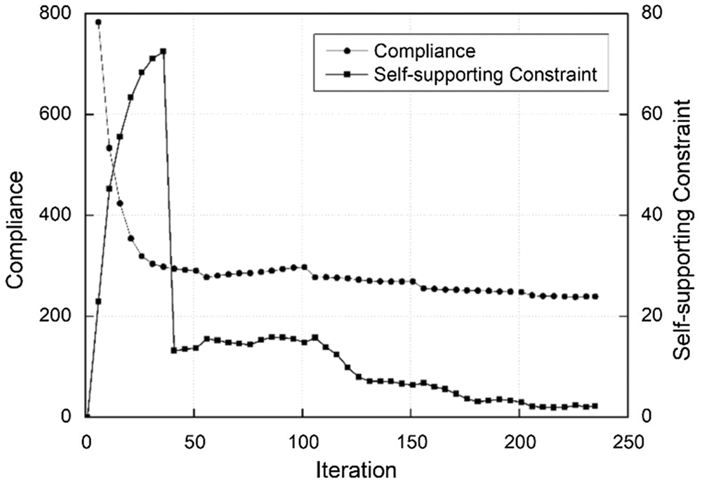
Figure 7: Convergence curves of compliance and self-supporting constraint
To illustrate the evolution of structural boundaries, the main unsupported structures are indicated by red ellipses, and the moving directions are indicated by red arrows, as shown in Fig. 6. As can be seen from these results, the boundaries of the unsupported structures move gradually to the baseplate with the increase of iteration steps.
To illustrate the final result more clearly, the COA is marked by red dash lines. It can be noted that the self-supporting constraint becomes active in the final design, which indicates the validity of the proposed method.
The iteration curve of compliance is quite stable except for the fluctuations caused by the periodic increase of the Heaviside parameter β. Nevertheless, the fluctuations are very small by adopting the volume preserving Heaviside filter. However, the iteration curve of self-supporting constraint fluctuates in a large scale, which decreases significantly at iteration 40. The main reason for this is that the build direction has been assigned and self-supporting constraint is reevaluated. Besides, as the self-supporting constraint is imposed on the gradual density transition region at the structural boundary, which leads to a certain degree of fluctuations with the evolution of structural configuration. Nevertheless, the fluctuations are insignificant in the later period of optimization, which is mainly attributed to the triangular directional sensitivity filter. As the structural configuration eventually becomes clear, the constraint values become stable as well.
To investigate the effect of parameter δ on the solutions, the MBB beam is optimized with δ of 0.3, 0.5, 0.7, and 0.9, respectively. The values of all other parameters are the same as before. All optimizations are converged, and the final build directions are all in orientation R. For comparison, the solutions are rotated 90° clockwise, as shown in Fig. 8, where the elements in red indicate the structural boundaries that cannot be successfully printed. As suggested by these results, the constraint value
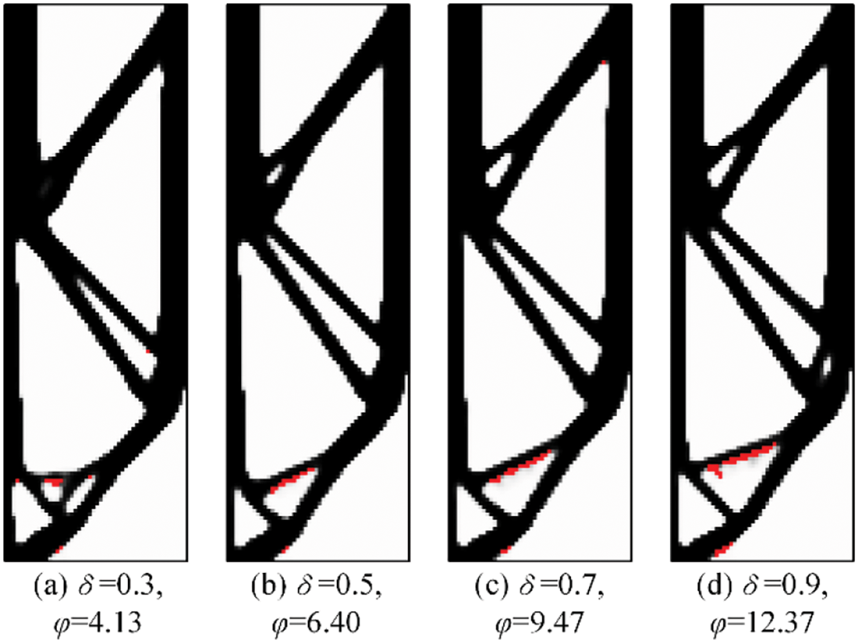
Figure 8: Optimum solutions for the MBB beam for different values of δ
In order to fully demonstrate the performance and robustness of the proposed algorithm, the optimizations with varying filter radius and COA are studied. In general, the optimization with large COA is hard to converge as the manufacturing constraint becomes very stringent, while high overhang angles are usually easy to print. For simplicity but without the loss of generality, a parameter study for 30°–60° is performed. The MBB beam is solved with filter radius R of 3.5 and 4.5 and COA of 30°, 45°, and 60°. The performance of the proposed method in maintaining the structural performance is measured by compliance ratio, c/cref, which is the structural compliance computed with or without self-supporting constraint.
All optimizations converged and realized self-supported successfully, with the optimized solutions and performances shown in Fig. 9, in which the baseplate is also presented by green blocks. It can be seen that the final build direction varies with different COAs, which is natural as the COA has direct influence on the constraint value
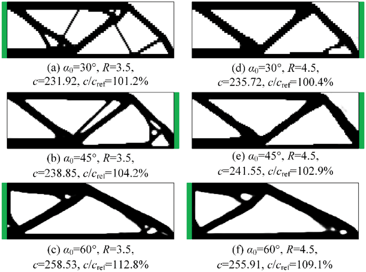
Figure 9: Optimum solutions for the MBB beam with various COAs and filter radiuses
As can be seen in Fig. 9, the compliance ratio c/cref is much smaller than the results in [35], which validates the effectiveness of the proposed TO procedure combined with build direction assignment. As expected, the result obtained when COA = 30° and filter radius is 3.5 is almost the same as the freely optimized result shown in Fig. 5. With the increase of COA, the constraint becomes stricter and makes the solutions deviate significantly from the free design results, which leads to greater performance loss. In addition, it can be noticed that the elements size with COA = 30° is larger than that of 60°. The reason for this is that the values of element height b are different. As the width a of elements is fixed to unit length, the elements height b is
The second case is a cantilever beam problem with two subcases, as shown in Fig. 10. The design domain is a 150 × 50 rectangular area, while in the general domain at right there is a prescribed circular hole at the center of design domain. Both models are fixed on the left edge with a unit external force exerted on the middle point of the right edge. The initial value of Heaviside projection parameter β is set to 0.25 and doubled every 50 iterations.
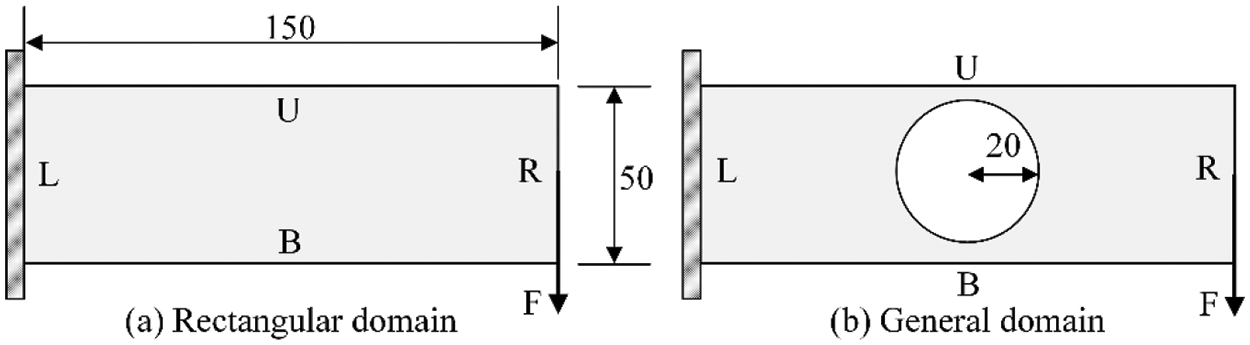
Figure 10: The design domain of cantilever beam example
The two cases are both first optimized without the self-supporting constraint. The allowable volume fraction is set to 30%, and filter radius is set to 3.5. The results are depicted in Fig. 11, and the compliance is 275.74 and 307.89, respectively. The prescribed hole will provide a challenge for evolving self-supported structures, which is conducive to testing the weaknesses of the proposed method.
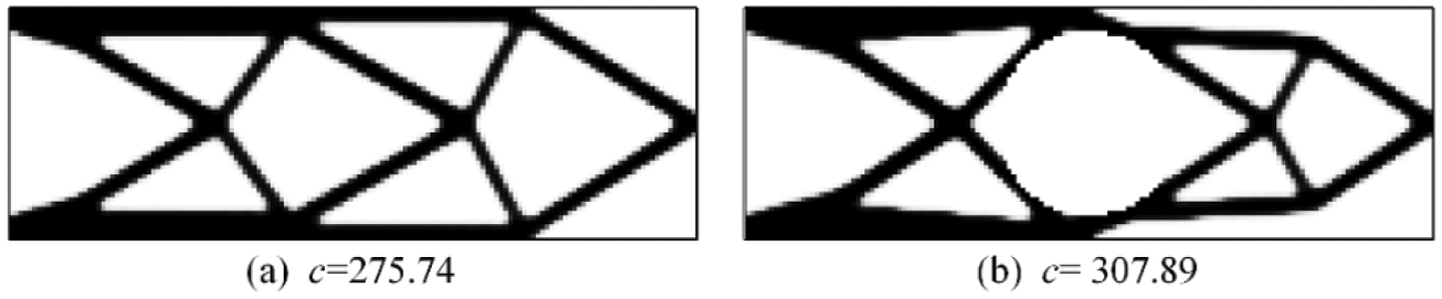
Figure 11: Optimum designs for the cantilever beam without self-supporting constraint
When the self-supporting constraint is considering, the COA is first set to 60°, while parameters
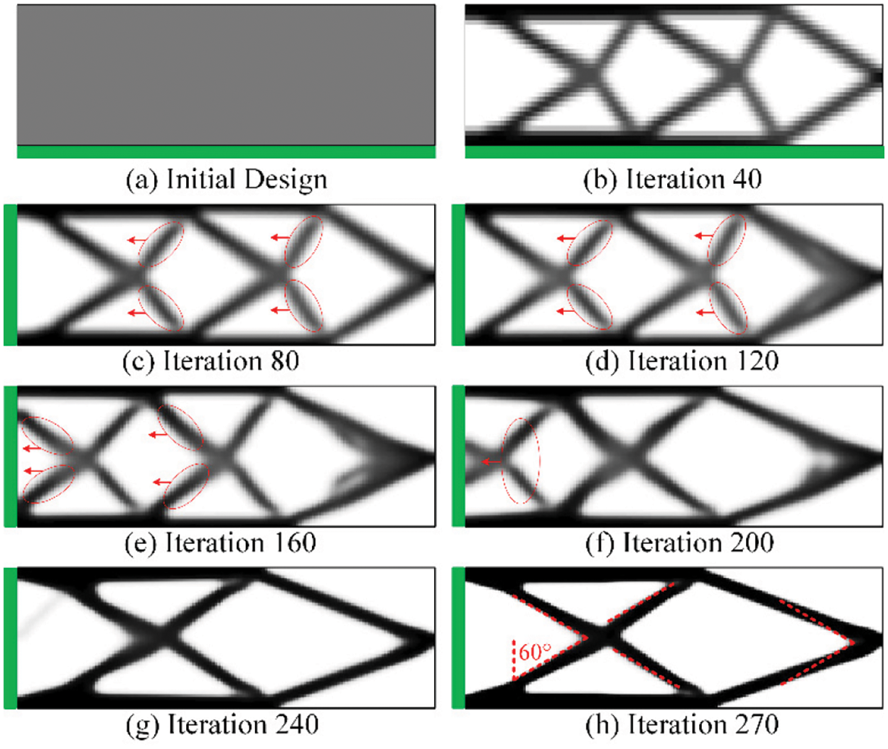
Figure 12: Design evolution history of the cantilever beam with self-supporting constraint
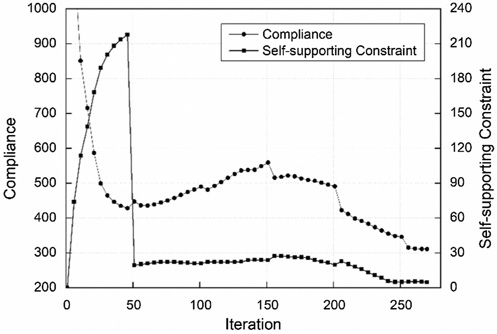
Figure 13: Convergence curves of compliance and self-supporting constraint
Similarly, the evolution of structural boundaries is indicated by red ellipses and red arrows, while the COA is marked by red dash lines. As can be seen from these results, the unsupported structures move toward to the baseplate gradually until the structure becomes fully self-supported. Compared with the reference design, the number of staggered structures is smaller and the structural layout is clean and simple.
It can be noted in Fig. 13 that the fluctuating range of compliance curve is much higher compared with the MBB example. The reason is that the structure configuration changes a lot as compared to the free design results. Besides, there are many intermediate density elements created during the evolution of structural boundaries due to the move limit. The build direction is assigned at iteration 47, which successively results in a significant reduction in self-supporting constraint value. It can be found out that the structural layout at iteration 40 is almost the same as the optimum design in Fig 11a except that there are more intermediate density elements.
Like the first example, the rectangular domain case is also optimized with δ of 0.3, 0.5, 0.7, and 0.9, respectively. All optimizations converged, and the print direction are all in orientation R. Similarly, all solutions are rotated 90° clockwise, as shown in Fig. 14. According to this figure, with the increase of δ, the number of unsupported elements increases and the constraint value
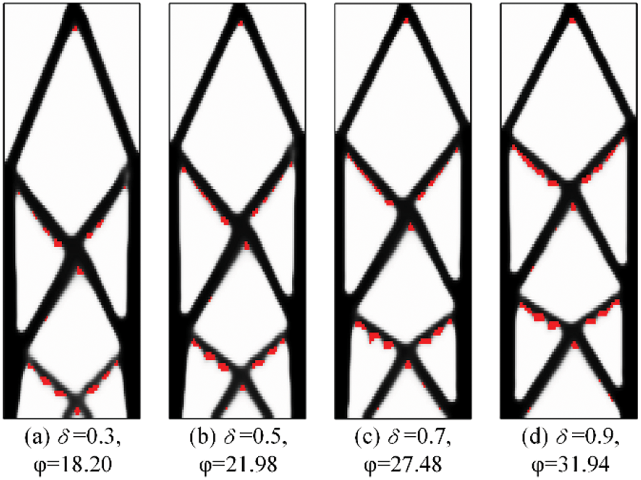
Figure 14: Optimized solutions for the cantilever beam for different values of δ
In order to fully demonstrate the performance and robustness of the proposed algorithm, the rectangular domain case is also solved with a filter radius of 2.5 and 3.5 and a COA of 30°, 45°, and 60°. All optimizations realize self-supported successfully, with the results shown in Fig. 15. It can be seen that all build directions are in in orientation L. With the increase of COA, the structural configuration changes more significantly compared with the free design result, and lead to a more significant performance loss. As expected, the result of COA = 30° is most similar to the freely optimized result. The influence of filter radius on structure configuration is less obvious than the first example. Nevertheless, a larger number of intermediate density elements can be noticed at structure boundaries for the filter radius of 3.5.
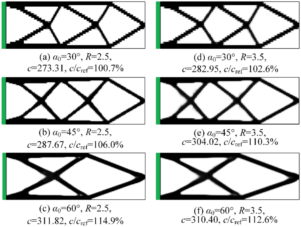
Figure 15: Optimum solutions for the rectangular domain with various COAs and filter radiuses
In addition, the cantilever beam with non-designable hole is solved with a COA of 30°, 45°, and 60° and an allowable volume fraction of 30% and 40%. The values of all other parameters are the same as before. The solutions are shown in Fig. 16. It can be seen from the figure that all solutions are self-supported, and the final build direction is in L orientation. With the increase of volume fraction, the structural compliance c decreases in a large extent as more elements can be used for load transfer. Besides, like in the previous cases, the structural configurations change more significantly compared with the free design results for larger COA, which leads to greater performance loss. The results demonstrate that the proposed method is effective in dealing with the structures containing non-designable domains.
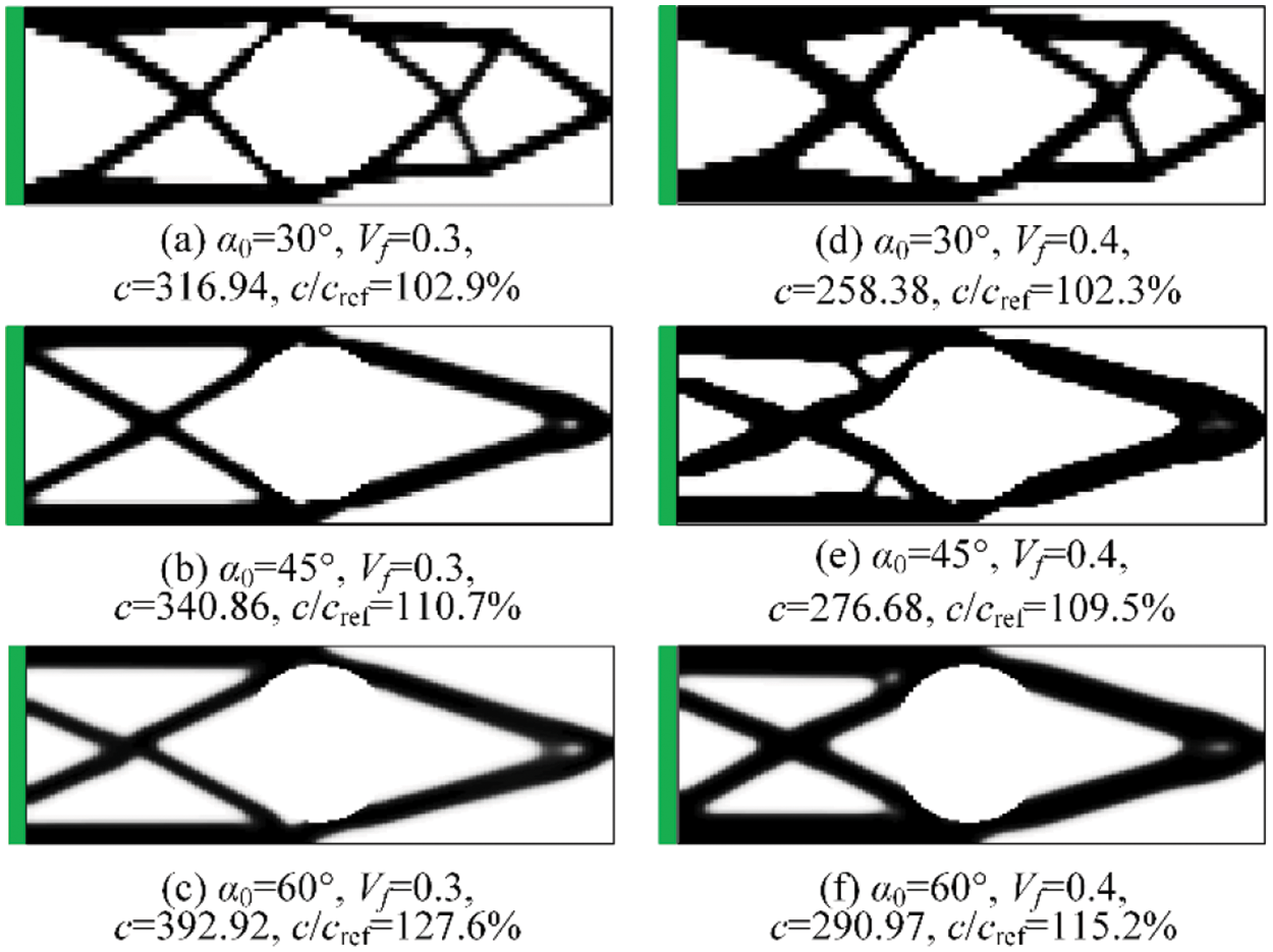
Figure 16: Optimum solutions for the general domain with various COAs and volume fractions
From the results as mentioned above, it can be found out that there are barely tiny or distorted structures in the solutions with self-supporting constraint. This is mainly attributed to the adaptive explicit continuous constraint, which realizes self-supported through the gradual evolution of supporting structures, and self-supported is only required at the final convergence point. The structural layouts are natural and clean, which has a significant meaning in improving manufacturability and alleviating stress concentration.
In this article, a TO procedure of self-supporting structures that suitable for various COA is proposed, which is integrated with build direction assignment to reduce performance loss caused by self-supporting constraint. Besides, a new adaptive explicit continuous self-supporting constraint function is constructed to quantify the degree of self-supporting constraint violation, which can be adaptively activated and tightened during the optimization process. In order to apply it to different COAs and build directions, the design domain is discretized with rectangular elements in a way that the element aspect ratio can be automatically altered. Besides, the volume preserving Heaviside projection filter is adopted to improve stability, and a triangular directional self-supporting constraint sensitivity filter is devised to promote the evolution of supporting structures and maintain stability.
Two numerical examples are presented to demonstrate the functionality and performance of the developed optimization procedure. All of the test cases have successfully converged and achieved self-supported, and the optimized solutions show good manufacturability. With the increase of COA, results show that the structural configuration changes more significantly compared with the result of free design, which leads to more severe performance loss. Nevertheless, by combining the TO optimization process with build direction assignment, the performance loss is reduced in a large extent.
In the future works, we will focus on extending the proposed method to 3D problems, and one of the main challenges is the computational efficiency. Besides, the definition of self-supporting criterion can be improved for unstructured meshes, so that the topology optimization can be performed in arbitrary build direction, and address complicated design cases.
Acknowledgement: The authors thank Krister Svanberg for the use of MMA optimizer.
Funding Statement: This work is supported by the National Key Research and Development Program of China (2018YFB1106303), and Scientific Research Foundation of CAUC (2017QD10S).
Conflicts of Interest: The authors declare that they have no conflicts of interest to report regarding the present study.
1. Liu, J., Gaynor, A. T., Chen, S., Kang, Z., Suresh, K. et al. (2018). Current and future trends in topology optimization for additive manufacturing. Structural and Multidisciplinary Optimization, 57(6), 2457–2483. DOI 10.1007/s00158-018-1994-3. [Google Scholar] [CrossRef]
2. Bendsoe, M. P., Kijuchi, N. (1988). Generating optimal topologies in structural design using a homogenization method. Computer Methods in Applied Mechanics and Engineering, 71(2), 197–224. DOI 10.1007/BF01650949. [Google Scholar] [CrossRef]
3. Bendsøe, M. P. (1989). Optimal shape design as a material distribution problem. Structural Optimization, 1(4), 193–202. DOI 10.1016/0045-7825(88)90086-2. [Google Scholar] [CrossRef]
4. Zhou, M., Rozvany, G. I. N. (1991). The COC algorithm, Part II: Topological, geometrical and generalized shape optimization. Computer Methods in Applied Mechanics and Engineering, 89, 309–336. DOI 10.1016/0045-7825(91)90046-9. [Google Scholar] [CrossRef]
5. Xie, Y. M., Steven, G. P. (1993). A simple evolutionary procedure for structural optimization. Computers & Structures, 49(5), 885–896. DOI 10.1016/0045-7949(93)90035-C. [Google Scholar] [CrossRef]
6. Wang, M. Y., Wang, X., Guo, D. (2003). A level set method for structural topology optimization. Computer Methods in Applied Mechanics and Engineering, 192, 227–246. DOI 10.1016/S0045-7825(02)00559-5. [Google Scholar] [CrossRef]
7. Guo, X., Zhang, W., Zhong, W. (2014). Doing topology optimization explicitly and geometrically—A new moving morphable components based framework. Journal of Applied Mechanics, 81(8), 081009. DOI 10.1115/1.4027609. [Google Scholar] [CrossRef]
8. Zhang, W., Chen, J., Zhu, X., Zhou, J., Xue, D. et al. (2017). Explicit three dimensional topology optimization via Moving Morphable Void (MMV) approach. Computer Methods in Applied Mechanics & Engineering, 322, 590–614. DOI 10.1016/j.cma.2017.05.002. [Google Scholar] [CrossRef]
9. Serphos, M. R. (2014). Incorporating AM-specific manufacturing constraints into topology optimization (Master's Thesis). Delft University of Technology. DOI 10.3990/1.9789036551496. [Google Scholar] [CrossRef]
10. Brackett, D., Ashcroft, I., Hague, R. (2011). Topology optimization for additive manufacturing. Proceedings of the 22nd Solid Freeform Fabrication Symposium, pp. 348–362. Austin. [Google Scholar]
11. Zhu, J., Zhou, H., Wang, C., Zhou, L., Yuan, S. et al. (2021). A review of topology optimization for additive manufacturing: Status and challenges. Chinese Journal of Aeronautics, 34(1), 91–110. DOI 10.1016/j.cja.2020.09.020. [Google Scholar] [CrossRef]
12. Thomas, D. (2009). The development of design rules for selective laser melting (Ph.D. Thesis). University of Wales. [Google Scholar]
13. Wang, Y., Xia, J., Luo, Z., Yan, H., Sun, J. et al. (2020). Self-supporting topology optimization method for selective laser melting. Additive Manufacturing, 36, 101506. DOI 10.1016/j.addma.2020.101506. [Google Scholar] [CrossRef]
14. Leary, M., Merli, L., Torti, F., Mazur, M., Brandt, M. (2014). Optimal topology for additive manufacture: A method for enabling additive manufacture of support-free optimal structures. Materials & Design, 63, 678–690. DOI 10.1016/j.matdes.2014.06.015. [Google Scholar] [CrossRef]
15. Gaynor, A. T., Guest, J. K. (2014). Topology optimization for additive manufacturing: Considering maximum overhang constraint. 15th AIAA/ISSMO Multidisciplinary Analysis and Optimization Conference, pp. 1–8. Atlanta, GA. [Google Scholar]
16. Gaynor, A. T., Guest, J. K. (2016). Topology optimization considering overhang constraints: Eliminating sacrificial support material in additive manufacturing through design. Structural and Multidisciplinary Optimization, 54, 1157–1172. DOI 10.1007/s00158-016-1551-x. [Google Scholar] [CrossRef]
17. Johnson, T. E., Gaynor, A. T. (2018). Three-dimensional projection-based topology optimization for prescribed-angle self-supporting additively manufactured structures. Additive Manufacturing, 24, 667–686. DOI 10.1016/j.addma.2018.06.011. [Google Scholar] [CrossRef]
18. Langelaar, M. (2016). Topology optimization of 3D self-supporting structures for additive manufacturing. Additive Manufacturing, 12, 60–70. DOI 10.1016/j.addma.2016.06.010. [Google Scholar] [CrossRef]
19. Langelaar, M. (2017). An additive manufacturing filter for topology optimization of print-ready designs. Structural and Multidisciplinary Optimization, 55(3), 871–883. DOI 10.1007/s00158-016-1522-2. [Google Scholar] [CrossRef]
20. Zhao, D., Li, M., Liu, Y. (2021). A novel application framework for self-supporting topology optimization. The Visual Computer, 37, 1169–1184. DOI 10.1007/s00371-020-01860-2. [Google Scholar] [CrossRef]
21. Qian, X. (2017). Undercut and overhang angle control in topology optimization: A density gradient based integral approach. International Journal for Numerical Methods in Engineering, 111(3), 247–272. DOI 10.1002/nme.5461. [Google Scholar] [CrossRef]
22. Wang, C., Qian, X. (2020). Simultaneous optimization of build orientation and topology for additive manufacturing. Additive Manufacturing, 34, 101246. DOI 10.1016/j.addma.2020.101246. [Google Scholar] [CrossRef]
23. van de Ven, E., Maas, R., Ayas, C., Langelaar, M., van Keulen, F. (2018). Continuous front propagation-based overhang control for topology optimization with additive manufacturing. Structural and Multidisciplinary Optimization, 57(5), 2075–2091. DOI 10.1007/s00158-017-1880-4. [Google Scholar] [CrossRef]
24. van de Ven, E., Maas, R., Ayas, C., Langelaar, M., van Keulen, F. (2020). Overhang control based on front propagation in 3D topology optimization for additive manufacturing. Computer Methods in Applied Mechanics and Engineering, 369, 113169. DOI 10.1016/j.cma.2020.113169. [Google Scholar] [CrossRef]
25. Garaigordobil, A., Ansola, R., Santamaria, J., Fernandez de Bustos, I. (2018). A new overhang constraint for topology optimization of self-supporting structures in additive manufacturing. Structural and Multidisciplinary Optimization, 58(5), 2003–2017. DOI 10.1007/s00158-018-2010-7. [Google Scholar] [CrossRef]
26. Zhang, K., Cheng, G., Xu, L. (2019). Topology optimization considering overhang constraint in additive manufacturing. Computers & Structures, 212, 86–100. DOI 10.1016/j.compstruc.2018.10.011. [Google Scholar] [CrossRef]
27. Luo, Y., Sigmund, O., Li, Q., Liu, S. (2020). Additive manufacturing oriented topology optimization of structures with self-supported enclosed voids. Computer Methods in Applied Mechanics and Engineering, 372, 113385. DOI 10.1016/j.cma.2020.113385. [Google Scholar] [CrossRef]
28. Mirzendehdel, A. M., Suresh, K. (2016). Support structure constrained topology optimization for additive manufacturing. Computer-Aided Design, 81, 1–13. DOI 10.1016/j.cad.2016.08.006. [Google Scholar] [CrossRef]
29. Liu, J., To, A. C. (2017). Deposition path planning-integrated structural topology optimization for 3D additive manufacturing subject to self-support constraint. Computer-Aided Design, 91, 27–45. DOI 10.1016/j.cad.2017.05.003. [Google Scholar] [CrossRef]
30. Zhang, W., Zhou, L. (2018). Topology optimization of self-supporting structures with polygon features for additive manufacturing. Computer Methods in Applied Mechanics and Engineering, 334, 56–78. DOI 10.1016/j.cma.2018.01.037. [Google Scholar] [CrossRef]
31. Wang, Y., Gao, J., Kang, Z. (2018). Level set-based topology optimization with overhang constraint: Towards support-free additive manufacturing. Computer Methods in Applied Mechanics and Engineering, 339, 591–614. 10.1016/j.cma.2018.04.040. [Google Scholar] [CrossRef]
32. Guo, X., Zhou, J., Zhang, W., Du, Z., Liu, C. et al. (2017). Self-supporting structure design in additive manufacturing through explicit topology optimization. Computer Methods in Applied Mechanics and Engineering, 323, 27–63. DOI 10.1016/j.cma.2017.05.003. [Google Scholar] [CrossRef]
33. Zhao, J., Zhang, M., Zhu, Y., Li, X., Wang, L. et al. (2019). A novel optimization design method of additive manufacturing oriented porous structures and experimental validation. Materials & Design, 163, 107550. DOI 10.1016/j.matdes.2018.107550. [Google Scholar] [CrossRef]
34. Wang, C., Zhang, W., Zhou, L., Gao, T., Zhu, J. (2021). Topology optimization of self-supporting structures for additive manufacturing with b-spline parameterization. Computer Methods in Applied Mechanics and Engineering, 374, 113599. DOI 10.1016/j.cma.2020.113599. [Google Scholar] [CrossRef]
35. Zou, J., Zhang, Y., Feng, Z. (2021). Topology optimization for additive manufacturing with self-supporting constraint. Structural and Multidisciplinary Optimization, 63, 2341–2353. DOI 10.1007/s00158-020-02815-w. [Google Scholar] [CrossRef]
36. Xu, S., Cai, Y., Cheng, G. (2010). Volume preserving nonlinear density filter based on heaviside functions. Structural and Multidisciplinary Optimization, 41(4), 495–505. DOI 10.1007/s00158-009-0452-7. [Google Scholar] [CrossRef]
37. Sigmund, O. (2007). Morphology-based black and white filters for topology optimization. Structural and Multidisciplinary Optimization, 33(4–5), 401–424. DOI 10.1007/s00158-013-0978-6. [Google Scholar] [CrossRef]
38. Svanberg, K. (1987). The method of moving asymptotes—A new method for structural optimization. International Journal for Numerical Methods in Engineering, 24, 359–373. DOI 10.1002/nme.1620240207. [Google Scholar] [CrossRef]
39. Andreassen, E., Clausen, A., Schevenels, M., Lazarov, B. S., Sigmund, O. (2011). Efficient topology optimization in MATLAB using 88 lines of code. Structural and Multidisciplinary Optimization, 43(1), 1–16. DOI 10.1007/s00158-010-0594-7. [Google Scholar] [CrossRef]
 | This work is licensed under a Creative Commons Attribution 4.0 International License, which permits unrestricted use, distribution, and reproduction in any medium, provided the original work is properly cited. |