| Computer Modeling in Engineering & Sciences |
DOI: 10.32604/cmes.2022.019781
ARTICLE
Dynamical Model to Optimize Student’s Academic Performance
Department of Mathematics, Near East University, Mersin, 10 KKTC, Cyprus
*Corresponding Author: Amna Hashim Alzadjali. Email: gtr-y2006@hotmail.com
Received: 14 October 2021; Accepted: 17 January 2022
Abstract: Excellent student’s academic performance is the uppermost priority and goal of educators and facilitators. The dubious marginal rate between admission and graduation rates unveils the rates of dropout and withdrawal from school. To improve the academic performance of students, we optimize the performance indices to the dynamics describing the academic performance in the form of nonlinear system ODE. We established the uniform boundedness of the model and the existence and uniqueness result. The independence and interdependence equilibria were found to be locally and globally asymptotically stable. The optimal control analysis was carried out, and lastly, numerical simulation was run to visualize the impact of the performance index in optimizing academic performance.
Keywords: Academic performance; optimal control; uniform boundedness; Pontryagin Maximum Principle (PMP); existence and uniqueness; stability
The human capital theory perceives education and learning activities as an investment in people to increase the productivity of goods and services [1]. The industrial and technological development of a country depends on literacy as a requirement for its success. This is especially when a literate member of society engages in an active and effective role in the development process. There is no doubt that combining the skills of improving income generation with knowledge of sustainable development assist mankind in improving his material condition of living through the use of resources available to him.
The academic performance of a student serves as the bedrock for knowledge acquisition and the development of skills that directly impact the socio-economic development of a country [2]. It determines the success or failure of any academic institution [3].
There are many factors that enhance and impede students’ academic performance attributed to students, parents, teachers and environments. The student’s factors include self- motivation, interest in a subject, punctuality in class, regular studying and access to learning materials. Class attendance and students’ attitudes toward their learning have an impact on academic performance. In [4], it is confirmed that in the case of mathematics, students’ attitude towards the subject has a direct impact on their academic performance.
Qualified teachers and facilitators render effective facilitation which enhances academic performance. However, performance target, completion of syllabus, paying attention to weak students, assignment and student evaluation have significant impact too [5].
Parental background and status have significant impact on student’s academic performance. Educated parent provide home school tutorial to their ward and are more encouraging as well. In [6], it was shown that, students with high level of parental involvement in their academics excel their counterparts with no such involvement.
Environmental factors that influence academic performance are enabling environment, infrastructure, adequate facilities and learning materials, well-equipped laboratories, etc. In [7], it is revealed that the availability of physical resources such as the library, textbooks, adequacy of classroom and spacious playing ground affect the performance of the students. Reference [8] emphasized that the use of instructional equipment facilitates effective service delivery and enhances teaching and learning. Distanced school also affects students’ performance in the sence that the more school distance, the more tired students become [9,10].
Also, fairly disciplined schools perform better than less or no disciplined schools. Effective discipline is used to control students’ behavior, which has a direct impact on their academic performance [11]. Furthermore, the student-to-teacher ratio or class size also affects performance. Effective teaching in a moderate class ratio enhances performance [12].
Age has a significant impact on academic performance; older students are likely to drop out than younger ones. Reference [10] showed a significant positive impact of age on academic performance in mathematics and science but the degree of the association is weak.
Mathematical models play a significant role in solving real-life problems [13–15]. Moreover, a mathematical model is an important tool used to optimize a real-life problem for the quickest and effective resolution [16–20]. In this paper, we study the uppermost priority and goal of educators and facilitators. The dubious marginal rate between admission and graduation rates unveils the rates of dropout and withdrawal from school. To improve the academic performance of students, we optimize the performance indices to the dynamics describing the academic performance in the form of nonlinear ODE.
The paper is arranged as follows: Introduction is given in chapter one, followed by definitions of terms and important theorems in Chapter two. Chapter three gives the detail of model formulation while Chapter four gives stability analysis of the solutions of the model. Chapter five is the detailed formation of optimal control and numerical simulations.
Definition 1: [21] (Optimal Control)
A fairly general continuous time optimal control problem can be defined as follows:
Problem i: To find the control vector trajectory
subject to:
where
Problem ii: Find
subject to:
This special type of optimal control problem is called the minimum time problem.
Definition 2: [21] (Hamiltonian)
With a time varying Largrange’s multiplier function
such that
Theorem 1: [22] (Banach’s Fixed Point Theorem)
Let
then there exists a unique fixed point
The above theorem states the conditions sufficient for the existence and uniqueness of a fixed point, which we will see in a point that is mapped to itself.
Theorem 2: [23] (Lyapunov Function Theorem)
Let
i)
ii)
Further,
Theorem 3: [24] (Pontryagin Maximum Principle)
If
such that, for almost all
and such that at terminal time
If the functions
This theorem is used in optimal control theory to find the best possible control for taking a dynamical system from one state to another, especially in the presence of constraints for the state or input controls.
Remark 1: [25] For a minimum, it is necessary for the stationary (optimality) condition to give:
The model is constructed based on the assumption that the new intake is admitted into the average class at the rate
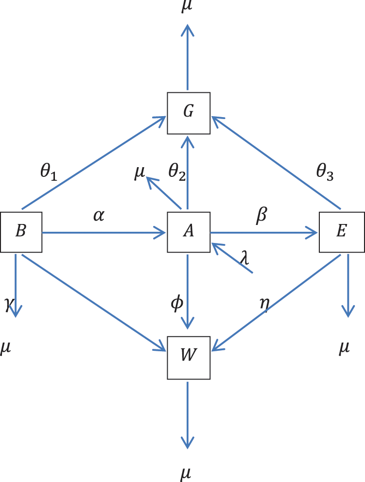
Figure 1: Schematic diagram describing the dynamics of student academic performance
The performance dynamics is described by the nonlinear system of ODE
Theorem 4: All the solutions of model are confined within bounded subset
Proof
Let the population size be
then
Solving the linear ODE (17) gives
The long-term behavior of (18) yield
Meanwhile, as time increases without bound all the solutions converge to the equilibrium
Theorem 5: The system (11)–(15) is Lipschitz continuous
Proof
Let the system (11)–(15) be of the form
where,
Analogously, we obtained
where
and
Composing the system (11)–(15) in vector form as
Since
Theorem 6: Let
Proof
Let
Since
Hence
Define the fixed point operator
So,
For contraction
Since
Since the state Eq. (15) depends on the previous states, it suffices to analyze (11)–(15).
The system (11)–(15) has the following equilibrium solutions
The independence equilibrium
and
where,
From system (11)–(15) we formulate the following Jacobian matrix, and then we test the equilibrium solution in the Jacobian matrix, if all the eigenvalues are negative, then the solution is locally stable, otherwise it is unstable [26,27].
Theorem 7: The independence equilibrium (
Proof
The eigenvalues of
For
and
Theorem 8: The independence equilibrium
Proof
Define
Since,
Then
The time derivative of
Applying the relation between arithmetic and geometric means:
Since,
then
Hence
Theorem 9: The interdependence equilibrium
Proof
Define
since,
then
The time derivative of
Applying the relation between arithmetic and geometric means:
Since,
Then
Hence
5 Formation of Optimal Control
The optimal control strategy is aimed at optimizing student’s academic performance which reflects in the increase of number of graduating students.
Let the control rates:
Then the control dynamics is described by the nonlinear system of ODE below:
subject to the objective functional;
where
We seek for optimal control
where
5.1 Characterization of Optimal Control
To derive the optimal academic performance of student, define Hamiltonian,
Theorem 10: Let
Proof
Applying (10),
Analogously,
and
subject to transversality condition as in [28,29]
Applying the optimality condition
Hence,
In this section numerical examples are given to support the analytic results. We use the following values of variables and parameters for the simulations. Fig. 2 compares the dynamics of different populations involved in the model. Figs. 3 and 4 compare the dynamics of the Weak student to the dynamics of Graduating student and then to the dynamics of Excellent students, respectively. Figs. 5–9 show the significance of the control on different populations involved in the model.
Fig. 2 depicts the dynamics of all the populations involved in the model. It can be seen that as only Graduate and Weak students reach and pass the fifth year indicating graduation and spillovers, respectively.
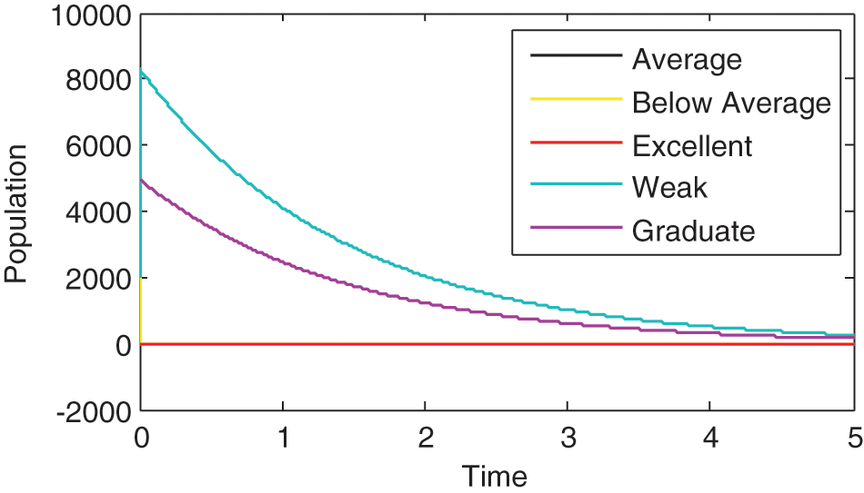
Figure 2: Dynamics of different populations in the model
Fig. 3 compares the dynamics of Graduate and Weak students. It can be seen that although both reach the fifth year, but Weak students’ population didn’t reach zero in the fifth year. This gives the possibility of spillovers. Also, since the population of Weak students is higher than that of Graduate students, there is need for taking appropriate measures to improve students learning.
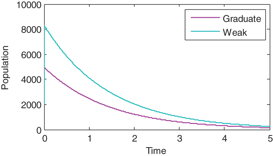
Figure 3: Comparison between dynamics of weak and graduate students
Fig. 4 compares the dynamics of Weak and Excellent students. Clearly the population of Weak students is higher. This is so true in most of our universities and colleges, excellent students have smallest population.

Figure 4: Comparison between dynamics of weak and excellent students
Fig. 5 compares the dynamics of Weak students with and without control. The effect of control is clearly seen. It is clear that, when appropriate control measures are taken, students’ performances can be improved and the number of graduate students can be increased.

Figure 5: Comparison between dynamics of Weak students with and without control
Fig. 6 compares the dynamics of Excellent students with and without control. The effect of control is clearly seen. It is clear that, when appropriate control measures are taken, Population of the Excellent students will be increased.

Figure 6: Comparison between dynamics of excellent students with and without control
Fig. 7 compares the dynamics of Average students with and without control. The effect of control is clearly seen. It is clear that, when appropriate control measures are taken, Population of the Average students will be increased.
Fig. 8 compares the dynamics of Below - Average students with and without control. The effect of control is clearly seen. It is clear that, when appropriate control measures are taken, the performance of Below Average students will be improved.
Fig. 9 compares the dynamics of Graduate students with and without control. The effect of control is clearly seen. It is clear that, when appropriate control measures are taken, the overall population of Graduate students will be increased. This is the ultimate target.

Figure 7: Comparison between dynamics of average students with and without control

Figure 8: Comparison between dynamics of below average students with and without control

Figure 9: Comparison between dynamics of graduating students with and without control
To improve the academic performance of students, we optimize the performance indices to the dynamics describing the academic performance in the form of nonlinear system ODE. We established the uniform boundedness of the model and the existence and uniqueness result. The independence and interdependence equilibria were found to be locally and globally asymptotically stable. The optimal control analysis was carried out, and lastly, numerical simulation was run to visualize the impact of the performance index in optimizing academic performance.
From the numerical simulation result, it can be observed that the weak students’ population dominates other populations. This shows that when there is too much intermingling between Weak students and the other categories of students, it will be to the disadvantage of the other students.
The significance of the optimal control is also clearly shown. There is a drastic increase in the populations of Average, below–Average, Excellent and Graduating students’ population after the application of the control. On the other hand, there is a drastic decrease in the population of weak students after the application of the control.
In the future, the fractional analogue of the model should be considered and real data should be used to validate it.
Funding Statement: The authors received no specific funding for this study.
Conflicts of Interest: The authors declare that they have no conflicts of interest to report regarding the present study.
1. Marginson, S. (2017). Limitations of human capital theory. Studies in Higher Education, 44(3), 1–15. DOI 10.1080/03075079.2017.1359823. [Google Scholar] [CrossRef]
2. Farooq, M. S., Chaudhry, A. H., Shafiq, M., Berhanu, G. (2011). Factors affecting students quality of academic performance: A case study of secondary school level. Journal of Quality and Technology Management, 7(2), 1–14. DOI 10.12691/education-3-12-13. [Google Scholar] [CrossRef]
3. Jayanthi, S. V., Balakrishnan, S., Ching, A. L. S., Latiff, N. A. A., Nasirudeen, A. M. A. (2014). Factors contributing to academic performance of students in a tertiary institution in Singapore. American Journal of Educational Research, 2(9), 752–758. DOI 10.12691/education-2-9-8. [Google Scholar] [CrossRef]
4. Peng, S. S., Hall, S. T. (1995). Understanding racial-ethnic differences in secondary school science and mathematics achievement. Research and Development Report. National Center for Education Statistics (EDU.S. Department of Education. Washington DC: ERIC. [Google Scholar]
5. Abubakar, A., Hilman, H., Kaliappen, N. (2018). New tools for measuring global academic performance. SAGE Open, 8(3), 1–10. DOI 10.1177/2158244018790787. [Google Scholar] [CrossRef]
6. Jeynes, W. H. (2002). Examining the effects of parental absence on the academic achievement of adolescents: The challenge of controlling for family income. Journal of Family and Economic, 23(2), 56–65. DOI 10.1023/A:1015790701554. [Google Scholar] [CrossRef]
7. Crosnoe, R., Johnson, M. K., Elder, G. H. (2004). School size and the interpersonal side of education: An examination of race/ethnicity and organizational context. Social Science Quarterly, 85(5), 1259–1274. DOI 10.1111/j.0038-4941.2004.00275.x. [Google Scholar] [CrossRef]
8. McCoy, L. P. (2005). Effect of demographic and personal variables on achievement in eighth grade algebra. Journal of Educational Research, 98(3), 131–135. DOI 10.3200/JOER.98.3.131-135. [Google Scholar] [CrossRef]
9. Eamon, M. K. (2005). Social demographic, school, neighborhood and parenting influences on academic achievement of Latino young adolescents. Journal of Youth and Adolescence, 34(2), 163–175. DOI 10.1007/s10964-005-3214-x. [Google Scholar] [CrossRef]
10. Baliyan, S. P., Khama, D. (2020). How distance to school and study hours after school influence students’ performance in mathematics and english: A comparative analysis. Journal of Education and E-Learning Research, 7(2), 209–217. DOI 10.20448/journal.509.2020.72.209.217. [Google Scholar] [CrossRef]
11. Ehiane, S. (2014). Discipline and academic performance: A study of selected secondary school in lagos. International Journal of Academic Research in Progressive Education and Development, 3(1), 181–194. [Google Scholar]
12. Little, J. W. (2003). Inside teacher community: Representations of classroom practice. Teachers College Record, 105(6), 914–945. DOI 10.1111/1467-9620.00273. [Google Scholar] [CrossRef]
13. Qureshi, S., Yusuf, A., Shaikh, A. A., Inc, M., Baleanu, D. (2019). Fractional modeling of blood ethanol concentration system with real data application. Chaos: An Interdisciplinary Journal of Nonlinear Science, 29(1), 013143. DOI 10.1063/1.5082907. [Google Scholar] [CrossRef]
14. Yusuf, A., Qureshi, S., Inc, M., Aliyu, A. I., Baleanu, D. et al. (2018). Two–strain epidemic model involving fractional derivative with Mittag–Leffler kernel. Chaos: An Interdisciplinary Journal of Nonlinear Science, 28(12), 123121. DOI 10.1063/1.5074084. [Google Scholar] [CrossRef]
15. Qureshi, S., Yusuf, A. (2019). Modeling chickenpox disease with fractional derivatives: From Caputo to Atangana-Baleanu. Chaos, Solitons & Fractals, 122(5), 111–118. DOI 10.1016/j.chaos.2019.03.020. [Google Scholar] [CrossRef]
16. Baleanu, D., Sajjadi, S. S., Jajarmi, A., Defterli, O. (2021). On a nonlinear dynamical system with both chaotic and non-chaotic behaviours: A new fractional analysis and control. Advances in Difference Equations, 2021(1), 234. DOI 10.1186/s13662-021-03393-x. [Google Scholar] [CrossRef]
17. Cao, N., Zhang, H., Luo, Y., Feng, D. (2012). Infinite horizon optimal control for nonlinear interconnected large-scale dynamical systems with an application to optimal attitude control. Asian Journal of Control, 14(5), 1239–1250. DOI 10.1002/asjc.452. [Google Scholar] [CrossRef]
18. Baleanu, D., Sajjadi, S. S., Asad, J. H., Jajarmi, A., Estri, E. (2021). Hyperchaotic behaviors, optimal control, and synchronization of a nonautonomous cardiac conduction system. Advances in Difference Equations, 2021(1), 77. DOI 10.1186/s13662-021-03320-0. [Google Scholar] [CrossRef]
19. Effati, S., Sabberi Nik, H., Jajarmi, A. (2013). Hyperchaos control of the hyperchaotic Chen system by optimal control design. Nonlinear Dynamics, 73(1–2), 499–508. DOI 10.1007/s11071-013-0804-0. [Google Scholar] [CrossRef]
20. Jajarmi, A., Baleanu, D., Vahid, K. Z., Mobayen, S. (2021). A general fractional formulation and tracking control for immunogenic tumor dynamics. Mathematical Methods in the Applied Sciences, 45(2), 667–680. DOI 10.1002/mma.7804. [Google Scholar] [CrossRef]
21. Becerra, V. M. (2008). Optimal control. Scholarpedia, 3(1), 5354. DOI 10.4249/scholarpedia.5354. [Google Scholar] [CrossRef]
22. Banach, S. (1922). Sur les operations dans les ensembles et leur application aux equations integrals. Fundamental Mathematicae, 3(1), 133–181. DOI 10.4064/fm-3-1-133-181. [Google Scholar] [CrossRef]
23. Lyapunov, A. M. (1892). The general problem of stability of motion (Doctoral Dissertation). University of Kharkov. [Google Scholar]
24. Vinter, R. (2013). Optimal control and pontryagin’s maximum principle. Encyclopedia of systems and control. London: Springer. [Google Scholar]
25. Paul, K. (1980). The solution and sensitivity of a general optimal control problem. Applied Mathematical Modelling, 4(4), 287–294. DOI 10.1016/0307-904X(80)90197-3. [Google Scholar] [CrossRef]
26. Singh, H., Srivastava, H. M., Hammouch, Z., Nisar, K. S. (2021). Numerical simulation and stability analysis for th3.1e fractional order dynamics of COVID–19. Results in Physics, 20(23–24), 103722. DOI 10.1016/j.rinp.2020.103722. [Google Scholar] [CrossRef]
27. Ngoc, T. B., Tri, V. V., Hammouch, Z., Can, N. H. (2021). Stability of a class of problems for time-space fractional pseudo-parabolic equation with datum measured at terminal time. Applied Numerical Mathematics, 167(7), 308–329. DOI 10.1016/j.apnum.2021.05.009. [Google Scholar] [CrossRef]
28. Area, I., Ndairou, F., Nieto, J. J., Silva, C. J., Torres, D. F. M. (2018). Ebola model and optimal control with vaccination constraints. Journal of Industrial & Management Optimization, 14(2), 427–446. DOI 10.3934/jimo.2017054. [Google Scholar] [CrossRef]
29. Elhia, M., Rachik, M., Benlahmar, E. (2013). Optimal control of an SIR model with delay in state and control variables. International Scholarly Research Notices, 2013, 403549. [Google Scholar]
 | This work is licensed under a Creative Commons Attribution 4.0 International License, which permits unrestricted use, distribution, and reproduction in any medium, provided the original work is properly cited. |