| Computer Modeling in Engineering & Sciences |
DOI: 10.32604/cmes.2022.019996
ARTICLE
State Estimation of Regional Power Systems with Source-Load Two-Terminal Uncertainties
1School of New Energy and Power Engineering, Lanzhou Jiaotong University, Lanzhou, 730070, China
2School of Electrical Engineering, Xi’an University of Technology, Xi’an, 710048, China
3School of Automation and Electrical Engineering, Lanzhou Jiaotong University, Lanzhou, 730070, China
*Corresponding Author: Shuaibing Li. Email: shuaibingli@mail.lzjtu.cn
Received: 28 October 2021; Accepted: 03 December 2021
Abstract: The development and utilization of large-scale distributed power generation and the increase of impact loads represented by electric locomotives and new energy electric vehicles have brought great challenges to the stable operation of the regional power grid. To improve the prediction accuracy of power systems with source-load two-terminal uncertainties, an adaptive cubature Kalman filter algorithm based on improved initial noise covariance matrix Q0 is proposed in this paper. In the algorithm, the Q0 is used to offset the modeling error, and solves the problem of large voltage amplitude and phase fluctuation of the source-load two-terminal uncertain systems. Verification of the proposed method is implemented on the IEEE 30 node system through simulation. The results show that, compared with the traditional methods, the improved adaptive cubature Kalman filter has higher prediction accuracy, which verifies the effectiveness and accuracy of the proposed method in state estimation of the new energy power system with source-load two-terminal uncertainties.
Keywords: New energy source; impact load; new energy power system; state estimation; uncertain system
Nomenclature
| EV : | Electric vehicles |
| EKF : | Extended Kalman filter |
| UKF : | Unscented Kalman filter |
| CKF : | Cubature Kalman filter |
| ACKF : | Adaptive cubature Kalman filter |
| IACKF : | Improved adaptive cubature Kalman filter |
| AP : | Affinity propagation |
| EMU : | Electric multiple units |
| AC : | Alternating current |
| DC : | Direct current |
| Q : | Noise covariance matrix |
| Q0 : | Traditional process noise covariance matrix |
| PMU : | Phase measurement unit |
| RMSE : | Root mean squared error |
The Hexi/Gansu corridor of China is rich in wind power and photovoltaic resources. The installed capacity of wind farms and photovoltaic power stations has increased significantly in recent years. By 2020, the total installed capacity of new energy in this region reached 23.69 million kW, contributing the most significant part of the new energy power source for the Gansu power grid. The total installed capacity of the new energy accounts for 42% of the entire amount in Gansu. Access to a high proportion of renewable energy improves the energy structure, bringing strong randomness and volatility. With the advancement of electric energy substitution and carbon neutralization goals, impact loads such as electric vehicles (EV) also increase and bring strong uncertainty to the stable operation of the power system. Therefore, accurately estimating the state of the source-load two-terminal uncertain systems is the premise of the planning, operation, and regulation of the new energy power system [1].
The cities, Jiuquan and Jiayuguan, have the largest million kW class of new energy demonstration bases in China and the leading Chinese steel and iron company. Additionally, these two cities are also the route of the Chinese trunk railway, the “Lanzhou-Xinjiang High-Speed Railway”, which makes the power supply network in this area a typical “source-load” two-terminal uncertain power system. With the continuous promotion of western development and the completion of the high-speed railway connecting the main road of the Lanzhou-Xinjiang High-Speed Railway in the northwest, the impact load capacity of electric locomotives has been increasing. At the same time, the new energy equipment manufacturing industry and the market ownership of new energy electric vehicles in the region have developed rapidly in recent years. The high proportion of large-scale wind power, photovoltaic, and other uncertain power sources and impact loads leads to large fluctuations in typical operation parameters, e.g., the voltage amplitude and the phase of the power grid, which puts forward higher requirements and new challenges for system state prediction, reliability of power grid dispatching, and stable operations of the power grid [2].
To keep the regional power grid parameters within the specified range, it is usually necessary to estimate the state of the operating parameters, such as voltage amplitude, phase, and frequency in the system according to various measurement information [3–6]. Currently, the state estimation methods for power systems mainly include two categories: static estimation and dynamic estimation. Static estimation only determines the estimated value of the state quantity at a particular time according to the measured value. However, it cannot estimate or predict the state quantity the next time [7,8]. The dynamic state estimation is based on the motion equation and predicts the state through the measured values of the system parameters at the current time [9–12]. Recently, improved algorithms based on the Kalman filter became the mainstream methods for power system dynamic state estimation, such as extended Kalman filter, unscented Kalman filter, and cubature Kalman filter (CKF) [13–16]. Among them, the CKF has been well recognized for the dynamic state prediction of the power system given its numerical stability, free-of-weight parameter setting, and high filtering accuracy [17–19].
The access to a high proportion of new energy brings difficulties to power system predictions. Scholars have extensively studied the state estimation of the new energy power system [20–22]. They have solved the problem of low accuracy in the state estimation of the traditional power system using improved control technology and prediction algorithms. Considering the uncertainty of the new energy power system, including wind power, solar power, and other distributed generators, a probabilistic prediction method based on a superposition denoising automatic encoder is proposed for system state estimation [23]. To improve the estimation accuracy further, Wang et al. [24] proposed an adaptive cubature Kalman filter (ACKF) method for dynamic state estimation of a doubly-fed wind turbine, which improves the output power prediction accuracy when the wind turbine is running. Wang et al. [25] proposed a chaotic-radial basis function (RBF) prediction model, which realizes the accurate prediction of photovoltaic output.
The above research lays a foundation for the state prediction of a new energy power system. The randomness and fluctuation of load in the regional power grid have increased in recent years. Therefore, to deal with the problem of power system instability caused by such impacts, Liu et al. [26] proposed a set of transient evaluation indexes to clarify the effect of different impact loads on the power grid. Meanwhile, Che et al. [27–29] realized a more accurate description of variables by improving the Latin hypercube sampling algorithm, conveniently providing relevant analysis and power flow calculation with load fluctuation.
There have been many studies of the characteristic analysis and prediction of source load single terminal uncertain systems at home and abroad. The state estimation of power systems with source-load two-terminal uncertainties has also received continuous attention. Considering the uncertainty of source-load terminals, Wei et al. [30] proposed a power grid planning flexibility evaluation method based on affinity propagation clustering and two-stage robust optimization. To consider the impact of source-load uncertainty on the power flow of the distribution network, the uncertainties of solar irradiation, wind speed, and load variation are studied [31]. The uncertainty probability density is modeled based on nuclear density estimation and is verified in different test systems.
Studies on state estimation of power systems integrated with new energy have been carried out for a long time, but publications on the state prediction of new energy power systems with two-side uncertainties are rarely reported. The problem of uncertainties exists in both the source and load sides, becoming more prominent. Therefore, this paper proposes a new method for state estimation of a new energy power system based on improved adaptive cubature Kalman filter (IACKF). The main innovations of this paper include the following points:
(1) The consideration of the randomness and fluctuation of wind and solar power generation, as well as the impact and instability of various impact loads, which can introduce uncertainties in state estimation of power grid parameters;
(2) On the basis of the uncertain nature of both the power sources and the impact loads, improvement of the initial covariance of the IACKF significantly promotes the estimation accuracy of the system parameters; and
(3) The verification of the generality of this method in different scenarios based on the IEEE 30 node system.
The rest of this paper is organized as follows: First, the characteristics of a new energy power system with source-load two-terminal uncertainties are introduced. Then, the uncertainties in both the power source and the load side are modeled. Based on that, the state-space model of a new energy power system with source-load two-terminal uncertainties is established. Meanwhile, by analyzing the pros and cons of traditional methods in solving state-space equations, an IACKF algorithm is proposed. After that, verification of the effectiveness and accuracy of the proposed method is carried out and a conclusion is finally drawn.
2 Source-Load Uncertainties of the New Energy Power System
2.1 Structure and Characteristics of the New Energy Power System
Energy consumption is becoming more and more serious, and the environmental pollution caused by fossil fuel energy is further aggravated. It is necessary to increase the access capacity of renewable energy [32]. The large-scale integration of renewable energy, i.e., wind energy, solar energy, and other new energy, replaces traditional hydrothermal power generation. The randomness and uncertainty of wind and light make it more difficult to regulate the power side of the power system. At the same time, the development of large-scale industrial complexes, high-power traction loads (high-speed electric multiple units (EMUs), heavy haul trains), and electric vehicles (EVs) have continuously increased the impact and volatility of the load side. This leads to strong uncertainties in both the “source” and the “load” ends of the system, which have become the main characteristics of the new energy power system. The basic architecture of a new energy power system with source-load two-terminal uncertainties is shown in Fig. 1.
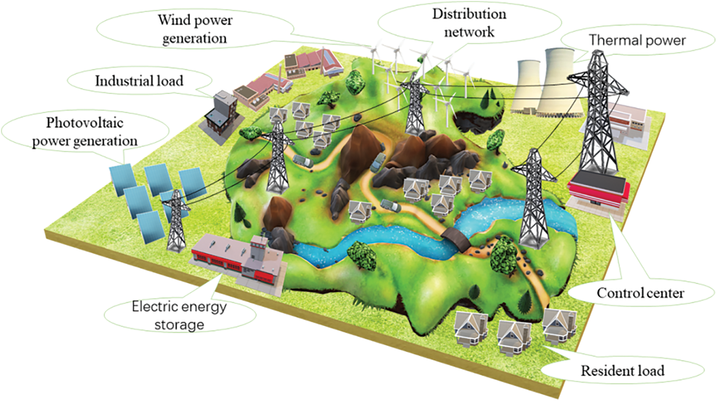
Figure 1: Schematic of the new energy power system
2.2 Randomness and Fluctuation in the Output of the Power Source Side
In the new energy power system, the uncertainties of the power source side are mainly reflected in the output of wind and photovoltaic power generation caused by the influence of wind, light, temperature, and other factors. The following part will introduce output characteristic modeling of the wind turbine, light, and other distributed generators in detail.
2.2.1 Probabilistic Modelling of Wind Turbine Output
The output power of wind turbines varies with the change of wind speed and relates to the environment of their installation location. To reflect the randomness of wind, Weibull distribution is generally used to describe wind speed [33]:
where f(v) is the distribution function of wind speed; v and ̅v are instantaneous and average values of wind speed; σv is the variance, depending on the prediction time scale.
The relationship between the output power of wind turbines and wind speed is as follows:
where Vin is the cut-in wind speed; VN is the rated wind speed; Vout is the cut-out wind speed; PN is the rated power.
2.2.2 Probabilistic Modelling of Photovoltaic Output
Usually, the light intensity is affected by atmospheric thickness, geographical location, meteorological climate and surface topography and has obvious temporal and spatial distribution characteristics. When the total amount of light intensity, H in a day, is constant, the ratio of light radiation in 24 h can be expressed by normal distribution [34]:
where, t∈ [1,24], d0 and d1 are constant coefficients; SL is the daily length; σR is the variance; R(t) is the ratio of radiation in each period to the total radiation in a day.
The hourly radiation is:
where H(t) is the hourly radiation of light intensity; H is the total amount of light intensity.
The peak watt-hour is the time when the sunshine intensity is 1000 W/m2, the temperature is 25°C, and the atmospheric quality is 1.5 standard atmospheric pressure:
where D(t) is the peak watt-hour; 0.0116 is the conversion coefficient.
where Ppeak and η are peak watt power and efficiency, respectively. WPV(t) is the hourly power generation of the photovoltaic battery pack.
2.3 Randomness and Uncertainties of Impact Loads
2.3.1 Load Characteristics of Electric Arc Furnace
The task of an electric arc furnace is to melt metal at high temperatures produced by electrode arc, which has great nonlinearity and impact on the regional distribution power grid. When connected to the power system, it will produce a large number of harmonics, resulting in voltage fluctuation and flicker, leading to negative sequence current, and so on.
Based on the law of energy conservation, with arc length and instantaneous current as the input of the model and arc conductance as the state variables, the arc energy equation is established as follows:
where R is the arc radius; I is arc current; K1, K2, K3, n, and m are variable parameters determined according to the actual situation.
According to Eq. (8), the arc conductance is:
whereas the arc resistance is:
2.3.2 Load Characteristics of Electric Rolling Mill
A rolling mill is a typical impact load in iron and steel enterprises. Its operation process includes four stages: preparation, no-load, biting, and rolling. When a single rolling mill in biting stage operates, its apparent power S1, active power P1, and reactive power Q1 can be calculated by Eqs. (11)
where cosφ1 is the power factor, Ku is the ratio of secondary line voltage of rectifier transformer to rated voltage; Ki is the ratio of primary line current of rectifier transformer to rolling mill current, Kt1 is the unit value of current under maximum operations mode, PNd is the rated power of rolling mill, ηNd is the rated efficiency, ηt is converter efficiency, m1 is the unit value of maximum torque, m1 = Kt1; ω1 is the unit value of speed, KCu is the active power loss coefficient, and D1 is the reactive power generated by the harmonic current.
In the rolling stage, the active, reactive, and apparent power P2, Q2, and S2 can be obtained similar to Eqs. (11)∼(13) by replacing P1, Q1, and S1 in the formula with P2, Q2, and S2.
2.3.3 Load Characteristics of the Electric Locomotive
An electric locomotive is the load unit of an electrified railway, including the high-speed EMU and the heavy haul traction train. The locomotive is supplied with the 25 kV AC power of the catenary. The electric arc can be frequently generated during operation due to the sliding electric contact among the catenary and the pantograph. This brings a large number of harmonics to the connected power grid. The mathematical model of its comprehensive load is as follows:
(1) The equation of state is:
(2) Power absorbed by load:
(3) Static load:
(4) Total active and reactive power:
where, E’, δ, and ω is the state variable; C is the capacitance; V is the voltage; V0 is the initial voltage; Tm is the mechanical torque; Ps0 is the initial value of static load active power; Qs0 is the initial value of static load reactive power; pv is the active power index; qv is reactive power index; ωr is rotor speed; ωv is synchronous speed; T′ is the transient time constant; M is the inertial time constant; X′ is transient reactance; X is synchronous reactance.
2.3.4 Load Characteristics of the Electric Vehicle
With the increasing number of EVs year by year, its typical impact load characteristics have become an essential factor affecting distribution network dispatching and operation control. The random charging time and space of EVs will have certain impacts on the stable operation of the power system and bring new uncertainty.
For an EV, the direct current (DC) charger as the core part is mainly composed of an alternating current/direct current (AC/DC) conversion link composed of an AC/DC rectifier and a direct current/direct current (DC/DC) high-frequency inverter link. The input impedance of its high-frequency power conversion circuit is:
where η is the efficiency of the power conversion module; U1 is the input power; I1 is the input current; P1 is the input power; Uo is the output power; Io is the output current; Po is output power.
The inductance and capacitance of power conversion are:
where ur is the equivalent voltage of the conversion circuit; id is the equivalent output current of the conversion circuit.
When the sine wave voltage U is added to R, take phase “a” as an example, the current and voltage can be denoted as:
where Sa(t) is the switching function of the diode:
3 State Estimation of the New Energy Power System
3.1 Application of Kalman Filter Algorithm in Power System State Estimation
3.1.1 Power System State Space Model
Generally, the power system, with dynamic characteristics, is described by the state-space model [35]:
where k is discrete-time; X(k) is the state of the system at the time k; Y(k) is the observation signal of the corresponding state at time k; W(k) is the input white noise; V(k) is the observation noise. Additionally, Eq. (23) is the equation of state and observation equation;
The two exponential smoothing method is used during state estimation to establish the system state equation, as shown in Eq. (24).
The voltage amplitude and phase are usually taken as a state variable, whereas the voltage amplitude and phase, active power and reactive power are taken as measurements, that is, x = [V θ]T, y = [P Q V θ]T.
where αH and βH is the smoothing parameter, and the value is between [0, 1].
3.1.2 The Cubature Kalman Filter
Based on the third-order spherical radial cubature criterion, the CKF uses a set of cubature points to approximate the state mean and covariance of nonlinear systems with additional Gaussian noise.
The basic steps of the CKF are consistent with other Kalman filter algorithms, which consists of two steps—prediction and update.
1) Prediction: according to the three-order spherical radial volume criterion, 2n equal weight points are obtained, and the state transition matrix is combined to solve the prior mean and variance of state variables.
Prediction steps are as follows:
First, calculate the cubature point:
of which:
Then, calculate the propagation cubature point:
Finally, calculate the prior mean and variance of the state quantity:
2) Update: update the predicted value and gain of state variables through measurements to obtain the posteriori mean and variance of state variables. The update steps are as follows:
First, calculate the cubature point:
Then, propagate the cubature point:
Finally, calculate the mean of measurements, error covariance, and cross-covariance:
and update gain, posteriori mean and variance:
3.1.3 Adaptive Cubature Kalman Filter
Although the CKF has a better performance than the Kalman filter, the prediction accuracy may be reduced due to the errors in the modeling process. Therefore, the noise estimator algorithm based on the fading memory exponential weighting method is introduced to update the Q at each time to adapt to the time variability of noise.
This method mainly forgets the effect of outdated data by emphasizing the influence of the latest data. It generates weighting coefficients for the next time noise influence, thus better approaching the time-varying noise, making the prediction algorithm better, time-variant, and accurate [36–38]. The estimation process of this method is as follows:
where b is the forgetting factor, and the value is 0 < b < 1; Kk is Kalman filter gain; Fk is the transfer matrix.
Since Q may lose its semi-positive nature in the operation process, the algorithm is ill-conditioned or cannot be calculated in the operation process. Therefore, the fault-tolerant algorithm recalculates Q in the case of non-positive semidefinite to ensure the positive semi-definite value of Q [39].
3.2 Improved Adaptive Cubature Kalman Filter
The traditional process noise covariance matrix, Q0, is the same as the measurement noise covariance matrix R0. This is mainly because Q0 comes from the voltage amplitude and phase measurement errors without considering the modeling error. In the new energy power system with source-load uncertainties, the state-space equation, established by the two exponential smoothing method, derives the state quantity from the state quantity. Therefore, it has certain accuracy only when the change of the power system is relatively stable. The state variables of the system with source-load uncertainties change greatly, and there is no apparent trend, so the accuracy of this modeling method is difficult to ensure. Therefore, this paper proposes to change the initial value of error covariance matrix Q to reduce the impact caused by inaccurate modeling and improve the prediction accuracy.
In the power system with source-load uncertainties, the ACKF algorithm works satisfactorily under appropriate Q and R. Therefore, selecting the appropriate value of Q0 has always been a great challenge. The process noise error of the state variable itself obeys the mean value of μ, and variance σ2, each state variable is independent of the other in the initial state, and the covariance is zero. Consequently, the initial error covariance matrix is taken as a diagonal matrix. According to the noise estimator of the fading memory index weighting method, the system error will change with the variation of the system operation state. The calculation process is as follows:
where d is the weighting coefficient, see Eqs. (33) and (34) for details.
For the power system with uncertainties in both source and load ends, the difficulty of the system state estimation is to accurately calculate the noise of each state quantity at each step. At time k, the average noise of voltage amplitude and phase of each system node is obtained. The noise obeys the mean value of zero and the variance of σk2. Since the error has a cumulative effect, the error at each step is accumulated, that is:
where n is the number of sampling points.
The above calculation is usually implemented for multiple systems to approximate the operation results. It can be obtained that the initial error Q0 of voltage amplitude follows the normal distribution with a mean value of zero and variance of 0.6, and the initial error of voltage phase angle follows the normal distribution, with a mean value of zero and variance of 0.08. The estimations of initial error Q0 are shown in Fig. 2. Once Q0 is introduced into the CKF algorithm with noise estimators, the estimated results can be readily obtained. The basic prediction steps are the same as the cubature Kalman filtering algorithm.
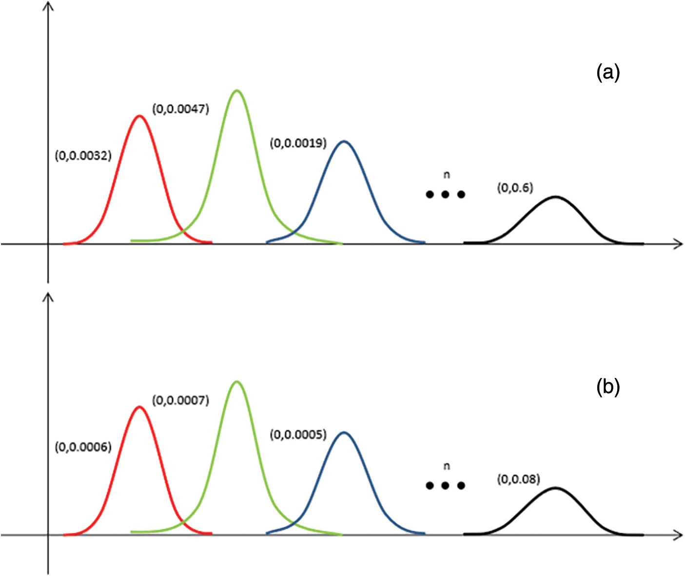
Figure 2: Estimations of initial error Q0: (a) voltage amplitude, (b) voltage phase angle
4 State Estimation of the New Energy Power System
4.1 Systematic Presentation of a Case Study
In this paper, the IEEE 30 node power system shown in Fig. 3 is adopted to verify the proposed method. Under different conditions, the equivalent wind and photovoltaic sources are connected to node B2. At the same time, the steel plant, EV, and traction locomotive are transformed according to the capacity ratio and connected to nodes B7, B8, and B21, respectively. The system operations data are collected every 10 min, and a total of 144 sampling points are obtained in one day. The true values of the state variables are obtained through power flow calculation, coupled with the measurement of Gaussian white noise, and the predicted values of the state variables of each node are obtained by using the ACKF. The phase measurement unit (PMU) is configured at Nodes 2, 4, 10, 12, 19, 24, and 27. The standard deviations of measurement error of supervisory control and data acquisition (SCADA), PMU voltage amplitude measurement error and the phase angle measurement error are 0.005, 0.02, and 0.002, respectively [40,41].
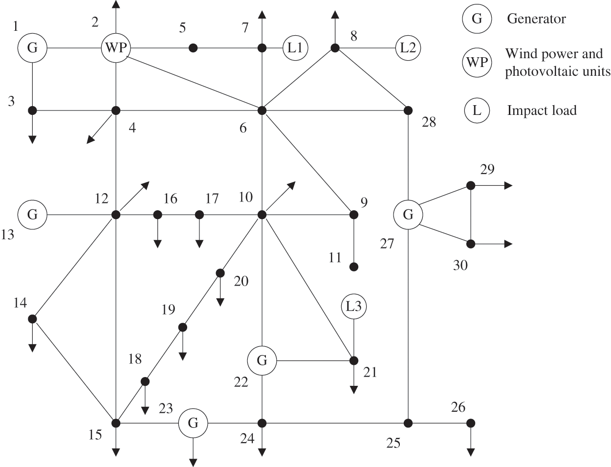
Figure 3: IEEE 30 node diagram
The mean square error is introduced as the performance index to quantitatively analyze the deviation between the estimated and the true value—the smaller, the better:
where N is the number of state variables, yk,i is the estimated value of the ith state variable, yk,it is the real value of the ith state variable.
4.2 The Construction of Simulation Scenario
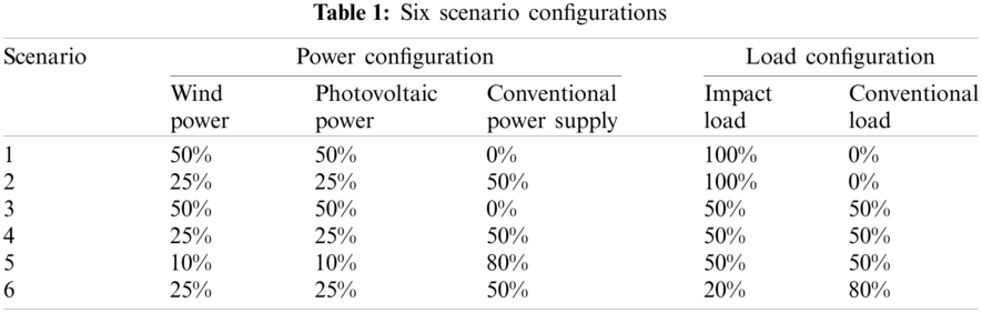
Assuming that the proportions of wind power, photovoltaic power, and impact load are 20%, 50%, and 100%, respectively, and combines different proportions of wind power, photovoltaic power and impact loads into six different scenarios. The uncertainty ratio from Scenario 1 to Scenario 6 decreases in turn. The scenario configuration is shown in Table 1.
4.3 The Analysis of Simulation
(1) Scenario 1
Wind power, photovoltaic power, and load are connected to different nodes. The wind turbine generator and photovoltaic power station are connected to Node 2, and the new energy power generation is 100% and connects the steel plant load, electric vehicle load, and electric traction locomotive load at Nodes 7, 8 and 21, respectively. The estimated value and mean square error of Node 9 are shown in Fig. 4.
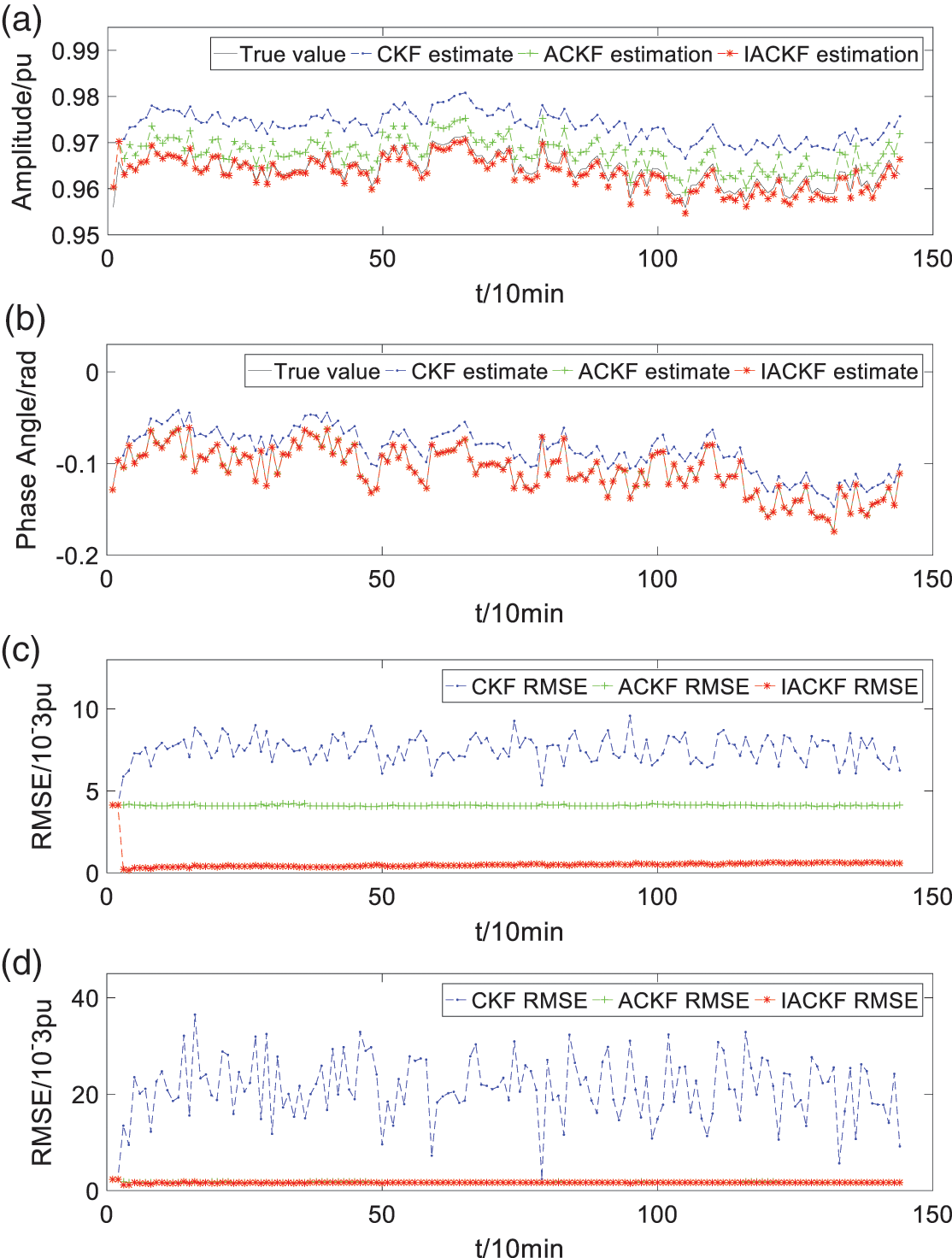
Figure 4: Estimation results of Scenario 1: (a) the true value and estimated value of the voltage amplitude of Node 9, (b) the true value and estimated value of the voltage phase angle of Node 9, (c) root mean squared error (RMSE) of voltage amplitude estimation, and (d) RMSE of voltage phase angle estimation
As can be seen from the Fig. 4, the variation range of voltage amplitude is about 0.9559~0.9715, IACKF has the best estimation effect, with a mean square error of about 0.53 × 10⁻³. The prediction effect of ACKF is the second, with a mean square error of about 4.11 × 10⁻³, and CKF has a poor prediction effect, with a mean square error of about 7.50 × 10⁻³. The variation range of voltage phase angle is approximately −0.1731~−0.0598, the mean square error of IACKF is roughly 1.63 × 10⁻³, the mean square error of ACKF is about 1.72 × 10⁻³, and the mean square error of CKF is 21.01 × 10⁻³.
(2) Scenario 2
The wind power and photovoltaic power are connected to Node 2, the traditional power supply is connected to other nodes, the new energy penetration rate is 50%, the wind power and photovoltaic account for 25%, respectively, and the load connected to the power grid is the same as Scenario 1. The estimated value and mean square error of Node 9 are shown in Fig. 5.

Figure 5: Estimation results of Scenario 2: (a) the true value and estimated value of the voltage amplitude of Node 9, (b) the true value and estimated value of the voltage phase angle of Node 9, (c) RMSE of voltage amplitude estimation, and (d) RMSE of voltage phase angle estimation
Voltage amplitude changes ranged from −0.9546 to 0.9716. The estimation effect of IACKF is about 0.43 × 10⁻³. The estimation effect of ACKF is approximately 4.10 × 10⁻³. The estimation effect of CKF is poor, and the mean square error is estimated at 6.72 × 10⁻³. Voltage phase angle changes ranged from −0.0316 to 0.0909. The mean square error of IACKF is about 1.66 × 10⁻³, the mean square error of ACKF is roughly 1.72 × 10⁻³, and the mean square error of CKF is approximately 18.25 × 10⁻³.
(3) Scenario 3
Wind and photovoltaic power account for 100%, and impact load accounts for 50% of the daily load. The estimated value and mean square error of Node 9 are shown in Fig. 6.

Figure 6: Estimation results of Scenario 3: (a) the true value and estimated value of the voltage amplitude of Node 9, (b) the true value and estimated value of the voltage phase angle of Node 9, (c) RMSE of voltage amplitude estimation, and (d) RMSE of voltage phase angle estimation
As shown in Fig. 6, the voltage amplitude range is −0.9699 to 0.9766. IACKF has the best prediction effect, with a mean square error of approximately 0.53 × 10⁻³. The estimation effect of ACKF is the second best, with a mean square error of roughly 4.21 × 10⁻³. CKF has a poor prediction effect, with a mean square error of about 5.02 × 10⁻³. The range of voltage phase angles is −0.1758 to −0.1018. The mean square error of IACKF, ACKF, and CKF is estimated at 1.68 × 10⁻³, 1.77 × 10⁻³, and 10.53 × 10⁻³, respectively.
(3) Scenario 4
The new energy penetration rate is 50%, the wind power and photovoltaic power account for 25%, respectively, and the impact load accounts for 50% of the daily load. The estimated value and mean square error of Node 9 are shown in Fig. 7.

Figure 7: Estimation results of Scenario 4: (a) the true value and estimated value of the voltage amplitude of Node 9, (b) the true value and estimated value of the voltage phase angle of Node 9, (c) RMSE of voltage amplitude estimation, and (d) RMSE of voltage phase angle estimation
The variation range of voltage amplitude is −0.9716~0.9796, IACKF has the best estimation effect, with the mean square error of approximately 0.45 × 10⁻³. The mean square error of ACKF is 4.20 × 10⁻³. The estimation effect of CKF is poor, with the mean square error of roughly 4.72 × 10⁻³. The variation range of voltage phase angle is −0.0437~0.0405. The mean square error of IACKF is estimated at 1.71 × 10⁻³, the mean square error of ACKF is 1.77 × 10⁻³, and the mean square error of CKF is about 9.29 × 10⁻³.
(5) Scenario 5
The new energy penetration accounts for 20%, the wind power and photovoltaic power account for 10%, respectively, and impact load accounts for 50% of the daily load. The estimated value and mean square error of Node 9 are shown in Fig. 8.
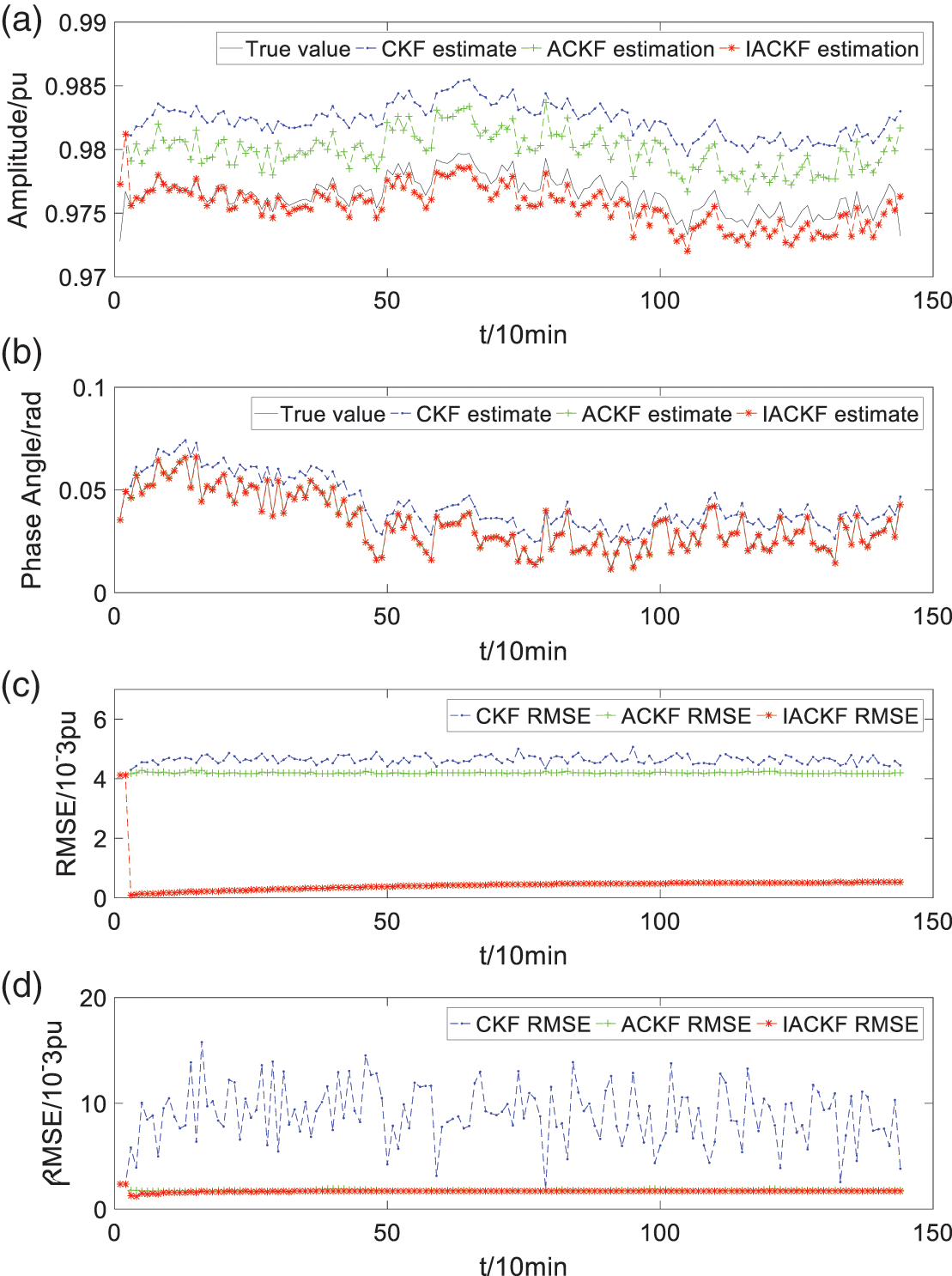
Figure 8: Estimation results of Scenario 5: (a) the true value and estimated value of the voltage amplitude of Node 9, (b) the true value and estimated value of the voltage phase angle of Node 9, (c) RMSE of voltage amplitude estimation, and (d) RMSE of voltage phase angle estimation
Voltage amplitudes vary from −0.9728 to 0.979. The mean square error of IACKF, ACKF, and CKF is estimated at 0.46 × 10⁻³, 4.19 × 10⁻³, and 4.63 × 10⁻³, respectively. Voltage phase angles vary from −0.0122 to 0.0671. The mean square error of IACKF is estimated at 1.70 × 10⁻³, the mean square error of ACKF is about 1.77 × 10⁻³, and the mean square error of CKF is approximately 8.91 × 10⁻³.
(6) Scenario 6
The new energy penetration accounts for 50%, the wind power and photovoltaic power account for 25%, respectively, and impact load accounts for 20% of the daily load. The estimated value and mean square error of Node 9 are shown in Fig. 9.

Figure 9: Estimation results of Scenario 6: (a) the true value and estimated value of the voltage amplitude of Node 9, (b) the true value and estimated value of the voltage phase angle of Node 9, (c) RMSE of voltage amplitude estimation, and (d) RMSE of voltage phase angle estimation
It can be seen from Fig. 9 that the variation range of voltage amplitude is −0.9776~0.9828. IACKF has the best estimation effect, with a mean square error of approximately 0.46 × 10⁻³. The mean square error of ACKF is roughly 4.26 × 10⁻³. CKF has a poor estimation effect, with a mean square error of about 4.28 estimation. The variation range of voltage phase angle is −0.0409~0.0214. The mean square error of IACKF is estimated at 1.72 × 10⁻³, the mean square error of ACKF is about 1.79 × 10⁻³, and the mean square error of CKF is 4.19 × 10⁻³.
From the estimated values of voltage amplitude and phase angles in different scenarios, the access of new energy and impulse load will significantly impact the stable operation of the power grid and the accuracy of algorithm prediction. The permeability of new energy and the proportion of impact load are different, and the voltage amplitude and phase angle fluctuation are also different. The first scenario with the highest proportion has significant fluctuation, and the fifth and sixth scenarios with the lowest proportion have small fluctuations.
Fig. 10 shows the mean square error of voltage and phase angle. As shown in this figure, the mean square error of voltage decreases with the uncertainty source load ratio decrease—the more stable the system, the more accurate the estimation. Respectively, in six scenarios, the average value of the IACKF algorithm is 0.5313 × 10⁻³, 0.4273 × 10⁻³, 0.53 × 10⁻³, 0.4457 × 10⁻³, 0.4561 × 10⁻³, and 0.4602 × 10⁻³, showing a downward trend as a whole, which is 93%, 94%, 89%, 90%, 90%, and 89% higher than thr CKF algorithm and 87%, 89%, 87%, 89%, 89%, and 89% higher than the ACKF algorithm. The IACKF algorithm has significant improvement in six scenarios compared with the other two algorithms. In the six scenarios where the uncertainty occupancy is gradually reduced, the accuracy of the CKF algorithm has a significant change, which is affected by large system fluctuations, and the algorithm is not stable enough. The ACKF algorithm is stable in six scenarios but has a significant estimation error. The IACKF algorithm has good estimation performance and high estimation accuracy in all scenarios.

Figure 10: Mean square error calculated by three algorithms in different scenarios. (a) Mean square error of voltage; (b) Mean square error of phase angle
The mean square error of the phase angle is similar to the mean square error of voltage. With the decrease of uncertainty source load ratio, the mean square error of the IACKF algorithm shows a downward trend. Respectively, in six scenarios the mean square error of IACKF algorithm is 1.6342 × 10⁻³, 1.6614 × 10⁻³, 1.6824 × 10⁻³, 1.7103 × 10⁻³, 1.7019 × 10⁻³, and 1.7205 × 10⁻³, which is 92%, 90%, 84%, 81%, 81%, and 59% higher than the CKF algorithm, and 5%, 4%, 4.7%, 3.2%, 4%, and 4.4% higher than the ACKF algorithm. The accuracy of the IACKF algorithm is much better than that of the CKF algorithm. Although the IACKF is not a significant improvement on the ACKF algorithm, it is slightly boosted in each scenario. Moreover, the IACKF algorithm does not change greatly with the change of uncertainty proportion and has a stable estimation ability compared with the CKF algorithm.
Therefore, the estimation effect of the IACKF algorithm is better than that of the CKF and ACKF algorithms, especially in voltage amplitude estimation, which shows that the IACKF can offset the influence of system noise caused by modeling error to a certain extent.
This paper is divided into six scenarios according to the different proportions of uncertain source loads connected to the power grid. The IACKF algorithm is used to estimate the state of six scenarios. The results show that the modeling error can be alleviated by changing the process noise error covariance matrix Q0. Compared with the CKF, the accuracy of the IACKF increased by approximately 90% and by roughly 88% compared with the ACKF. Compared with the CKF, the phase angle estimation was about 80% more accurate and around 4% more accurate than ACKF. Therefore, compared with the traditional CKF and ACKF, the IACKF had better prediction performance and accuracy.
Funding Statement: This work was supported by the Tianyou Youth Talent Lift Program of Lanzhou Jiaotong University, the Nature Science Foundation of Gansu (No. 21JR1RA255), the Gansu University Innovation Fund Project (Nos. 2020A-036 and 2021B-111).
Conflicts of Interest: The authors declare that they have no conflicts of interest to report regarding the present study.
1. Zhou, Y., Chen, J., Zhang, N., Zhang, Y., Teng, C. et al. (2021). Opportunity for developing ultra high voltage transmission technology under the emission peak, carbon neutrality and new infrastructure. High Voltage Engineering, 47(7), 2396–2408. DOI 10.13336/j.1003-6520.hve.20210203. [Google Scholar] [CrossRef]
2. Xiao, F., Yang, Z., Le, K., Wang, L., Duan, C. et al. (2021). Integrated energy storage system based on triboelectric nanogenerator in electronic devices. Frontiers of Chemical Science and Engineering, 15(2), 238–250. DOI 10.1007/s11705-020-1956-3. [Google Scholar] [CrossRef]
3. Zhang, G., Li, J., Cai, D., Huang, Q., Hu, W. (2021). Dynamic state estimation of power system with stochastic delay based on neural network. Energy Reports, 7(5), 159–166. DOI 10.1016/j.egyr.2021.02.009. [Google Scholar] [CrossRef]
4. Zhao, J., Gomez-Exposito, A., Netto, M., Mili, L., Abur, A. et al. (2019). Power system dynamic state estimation: Motivations, definitions, methodologies, and future work. IEEE Transactions on Power Systems, 34(4), 3188–3198. DOI 10.1109/TPWRS.2019.2894769. [Google Scholar] [CrossRef]
5. Chen, Y., Gao, Y., Zhao, J., Ge, L. (2021). Review on integrated energy system state estimation. High Voltage Engineering, 47(7), 2281–2292. DOI 10.13336/j.1003-6520.hve.20210362. [Google Scholar] [CrossRef]
6. Jovicic, A., Jereminov, M., Pileggi, L., Hug, G. (2020). Enhanced modelling framework for equivalent circuit-based power system state estimation. IEEE Transactions on Power Systems, 35(5), 3790–3799. DOI 10.1109/TPWRS.2020.2974459. [Google Scholar] [CrossRef]
7. Zheng, W., Wu, W., Gomez-Exposito, A., Zhang, B. (2016). Distributed robust bilinear state estimation for power systems with nonlinear measurements. IEEE Transactions on Power Systems, 32(1), 499–509. DOI 10.1109/TPWRS.2016.2555793. [Google Scholar] [CrossRef]
8. Hua, Y., Wang, N., Zhao, K. (2021). Simultaneous unknown input and state estimation for the linear system with a rank-deficient distribution matrix. Mathematical Problems in Engineering, 2021(12), 1–11. DOI 10.1155/2021/6693690. [Google Scholar] [CrossRef]
9. Chen, Y., Wang, Y., Yang, Q. (2021). Real-time state estimation method for distribution networks based on spatial-temporal feature graph convolution network. High Voltage Engineering, 47(7), 2386–2395. DOI 10.13336/j.1003-6520.hve.20210338. [Google Scholar] [CrossRef]
10. Liu, C., Li, Q., Wang, K. (2021). State-of-charge estimation and remaining useful life prediction of supercapacitors. Renewable and Sustainable Energy Reviews, 150(2), 111408. DOI 10.1016/j.rser.2021.111408. [Google Scholar] [CrossRef]
11. Langner, A., Abur, A. (2021). Formulation of three-phase state estimation problem using a virtual reference. IEEE Transactions on Power Systems, 36(1), 214–223. DOI 10.1109/TPWRS.2020.3004076. [Google Scholar] [CrossRef]
12. Yu, S., Fernando, T., Chau, T. K., Iu H. H. C. (2017). Voltage control strategies for solid oxide fuel cell energy system connected to complex power grids using dynamic state estimation and STATCOM. IEEE Transactions on Power Systems, 32(4), 3136–3145. DOI 10.1109/TPWRS.2016.2615075. [Google Scholar] [CrossRef]
13. Deng, Z., Shi, L., Yin, L., Xia, Y., Huo, B. (2020). UKF based on maximum correntropy criterion in the presence of both Intermittent observations and non-gaussian noise. IEEE Sensors Journal, 20(14), 7766–7773. DOI 10.1109/JSEN.2020.2980354. [Google Scholar] [CrossRef]
14. Guo, S., Wang, C., Chang, L., Zhou, J., Li, Y. (2020). Robust fading cubature Kalman filter and its application in initial alignment of SINS. Journal of Electrotechnics, 41(4), 95–101. DOI 10.1016/j.ijleo.2019.163593. [Google Scholar] [CrossRef]
15. Bi, T., Chen, L., Xue, A., Yang, Q. (2016). Dynamic state estimator for synchronous machines based on robust cubature Kalman filter. Journal of Electrotechnics, 31(4), 163–169. DOI 10.13334/j.0258-8013.pcsee.2014.16.022. [Google Scholar] [CrossRef]
16. Wang, K., Liu, C., Sun, J., Zhao, K., Wang, L. et al. (2021). State of charge estimation of composite energy storage systems with supercapacitors and lithium batteries. Complexity, 2021(15), 8816250. DOI 10.1155/2021/8816250. [Google Scholar] [CrossRef]
17. Luo, J., Fan, Y., Jiang, P., He, Z., Xu, P. et al. (2021). Vehicle platform attitude estimation method based on adaptive Kalman filter and sliding window least squares. Systems Engineering and Electronics, 32(3), 035007. DOI 10.1088/1361-6501/abc5f8. [Google Scholar] [CrossRef]
18. Liu, P., Xiang, Z., Jiang, Q., Geng, G., Sun, W. et al. (2019). Real-time dynamic state estimation for synchronous machines based on robust CKF. Power Grid Technology, 43(8), 2860–2868. DOI 10.13335/j.1000-3673.pst.2019.0247. [Google Scholar] [CrossRef]
19. Xu, W., Xu, J., Yan, X. (2020). Lithium-ion battery state of charge and parameters joint estimation using cubature Kalman filter and particle filter. Journal of Power Electronics, 20(1), 292–307. DOI 10.1007/s43236-019-00023-4. [Google Scholar] [CrossRef]
20. Liu, Y., Zhao, J., Xu, L., Liu, T., Qiu, G. et al. (2019). Online TTC estimation using nonparametric analytics considering wind power integration. IEEE Transactions on Power Systems, 34(1), 494–505. DOI 10.1109/TPWRS.2018.2867953. [Google Scholar] [CrossRef]
21. Chen, Y., Sun, H., Guo, Q. (2020). Energy circuit theory of integrated energy system analysis (VIntegrated electricity-heat-gas dispatch. Chinese Journal of Electrical Engineering, 40(24), 7928–7937. DOI 10.13334/j.0258-8013.pcsee.201715. [Google Scholar] [CrossRef]
22. Liu, C., Zhang, Y., Sun, J., Cui, Z., Wang, K. (2021). Stacked bidirectional LSTM RNN to evaluate the remaining useful life of supercapacitor. International Journal of Energy Research, 15(7), 1–10. DOI 10.1002/er.7360. [Google Scholar] [CrossRef]
23. Zhao, J., Mili, L., Gomez-Exposito, A. (2019). Constrained robust unscented Kalman filter for generalized dynamic state estimation. IEEE Transactions on Power Systems, 34(5), 3637–3646. DOI 10.1109/TPWRS.2019.2909000. [Google Scholar] [CrossRef]
24. Wang, T., Gao, M., Huang, S., Wang, Z. (2021). Dynamic state estimation for doubly fed induction generator wind turbine based on adaptive cubature Kalman filter. Power System Technology, 45(5), 1837–1845. DOI 10.13335/j.1000-3673.pst.2020.1389. [Google Scholar] [CrossRef]
25. Wang, Y., Fu, Y., Sun, L., Xue, H. (2018). Ultra-short term prediction model of photovoltaic output power based on Chaos-RBF neural network. Power System Technology, 42(4), 1110–1116. DOI 10.13335/j.1000-3673.pst.2017.2878. [Google Scholar] [CrossRef]
26. Liu, Z., Zhu, C., Wang, Y., Liu, J., Xie, P. (2017). Influence of impact load on transient characteristics of isolated power system. High Voltage Engineering, 43(10), 3443–3452. DOI 10.13336/j.1003-6520.hve.20170925036. [Google Scholar] [CrossRef]
27. Che, Y., Lv, X., Wang, X., Han, R. (2019). Improved two point estimation method for probabilistic power flow calculation with non-normal distribution. Power Automation Equipment, 39(12), 128–133. DOI 10.16081/j.epae.201912010. [Google Scholar] [CrossRef]
28. Han, R., Teng, Y., Xie, J., Wang, X., Che, Y. (2019). Identification of low-frequency oscillation in power system based on improved STD algorithm. Electric Power Automation Equipment, 39(3), 58–63. DOI 10.16081/j.issn.1006-6047.2019.03.009. [Google Scholar] [CrossRef]
29. Hu, Y., Wang, X., Teng, Y., Ai, P., Che, Y. (2019). Frequency stability control method of AC/DC power system based on multi-layer support vector machine. Proceedings of the CSEE, 39(14), 4104–4118. DOI 10.13334/j.0258-8013.pcsee.181496. [Google Scholar] [CrossRef]
30. Wei, L., Wang, W., Li, H., Xuan, W., Liu, Z. (2020). Evaluation on grid planning flexibility based on affinity propagation clustering and robust optimization. Proceedings of the CSU-EPSA, 32(3), 99–106. DOI 10.19635/j.cnki.csu-epsa.000387. [Google Scholar] [CrossRef]
31. Constante-Flores, G. E., Illindala, M. S. (2019). Data-driven probabilistic power flow analysis for a distribution system with renewable energy sources using monte Carlo simulation. IEEE Transactions on Industry Applications, 55(1), 174–181. DOI 10.1109/TIA.2018.2867332. [Google Scholar] [CrossRef]
32. Feng, X., Li, Q., Wang, K. (2021). Waste plastic triboelectric nanogenerators using recycled plastic bags for power generation. ACS Applied Materials & Interfaces, 13(1), 400–410. DOI 10.1021/acsami.0c16489. [Google Scholar] [CrossRef]
33. Zhou, Q., Wang, H., Wang, W. (2021). Modeling of wind speed probability distribution based on peak pattern identification. Acta Energiae Solaris Sinica, 42(8), 355–360. DOI 10.19912/j.0254-0096.tynxb.2019-0532. [Google Scholar] [CrossRef]
34. Qiu, Z., Sun, T., Liu, D., Yang, L., Xu, Z. (2021). Distribution characteristics of radiationin different meteorological conditionson various orientations in shenzhen. Acta Energiae Solaris Sinica, 42(5), 160–167. DOI 10.19912/j.0254-0096.tynxb.2019-1286. [Google Scholar] [CrossRef]
35. Netto, M., Mili, L. (2018). Robust data-driven Koopman Kalman filter for power systems dynamic state estimation. IEEE Transactions on Power Systems, 33(6), 7228–7237. DOI 10.1109/TPWRS.2018.2846744. [Google Scholar] [CrossRef]
36. Li, X., Huang, Z., Tian, J., Tian, Y. (2021). State-of-charge estimation tolerant of battery aging based on a physics-based model and an adaptive cubature Kalman filter. Energy, 220(2), 119767. DOI 10.1016/j.energy.2021.119767. [Google Scholar] [CrossRef]
37. Nugroho, S., Taha, A. F., Qi, J. (2019). Robust dynamic state estimation of synchronous machines with asymptotic state estimation error performance guarantees. IEEE Transactions on Power Systems, 35(3), 1923–1935. DOI 10.1109/TPWRS.2019.2949977. [Google Scholar] [CrossRef]
38. Jiang, K., Zhang, H., Karimi, H. R., Lin, J., Song, L. (2016). Simultaneous input and state estimation for integrated motor-transmission systems in a controller area network environment via an adaptive unscented Kalman filter. IEEE Transactions on Systems Man & Cybernetics Systems, 50(4), 1570–1579. DOI 10.1109/TSMC.2018.2795340. [Google Scholar] [CrossRef]
39. Wang, Y., Xia, M., Li, P., Guo, X., Bai, H. et al. (2020). Dynamic state estimation method of distribution network based on improved robust adaptive unscented Kalman filter. Automation of Electric Power Systems, 44(1), 92–100. DOI 10.7500/AEPS20190329004. [Google Scholar] [CrossRef]
40. Muscas, C., Pau, M., Pegoraro, P. A., Sulis, S. (2016). Uncertainty of voltage profile in PMU-Based distribution system state estimation. IEEE Transactions on Power Systems, 65(5), 988–998. DOI 10.1109/TIM.2015.2494619. [Google Scholar] [CrossRef]
41. Yu, S., Emami, K., Fernando, T., Lu, H. H. C., Wong, K. P. et al. (2016). State estimation of doubly fed induction generator wind turbine in complex power systems. IEEE Transactions on Power Systems, 31(6), 4935–4944. DOI 10.1109/TPWRS.2015.2507620. [Google Scholar] [CrossRef]
 | This work is licensed under a Creative Commons Attribution 4.0 International License, which permits unrestricted use, distribution, and reproduction in any medium, provided the original work is properly cited. |