| Computer Modeling in Engineering & Sciences |
DOI: 10.32604/cmes.2022.019715
ARTICLE
The Localized Method of Fundamental Solution for Two Dimensional Signorini Problems
1School of Civil Engineering and Architecture, Nanchang University, Nanchang, 330031, China
2Nanchang Institute of Technology, Nanchang, 330044, China
*Corresponding Authors: Anyu Hong. Email: honganyu@ncu.edu.cn; Fugang Xu. Email: xufugang785315056@126.com
Received: 10 October 2021; Accepted: 14 December 2021
Abstract: In this work, the localized method of fundamental solution (LMFS) is extended to Signorini problem. Unlike the traditional fundamental solution (MFS), the LMFS approximates the field quantity at each node by using the field quantities at the adjacent nodes. The idea of the LMFS is similar to the localized domain type method. The fictitious boundary nodes are proposed to impose the boundary condition and governing equations at each node to formulate a sparse matrix. The inequality boundary condition of Signorini problem is solved indirectly by introducing nonlinear complementarity problem function (NCP-function). Numerical examples are carried out to validate the reliability and effectiveness of the LMFS in solving Signorini problems.
Keywords: Signorini problem; localized method of fundamental solution; collocation method; nonlinear boundary conditions
In 1933, Signorini studied the frictionless contact problem between a linear elastic body and a rigid body. The related boundary condition is expressed by inequality constraints or complementary forms, which is also called the ambiguous boundary [1]. Fichera has proved the existence and uniqueness of the Signorini problem in 1964, and began to call this problem Signorini problem [2]. The theory of variational inequality was introduced for the first time in 1972, the existence and uniqueness of solution to Signoniri problem are discussed [3]. Later in 1985, Glowinski proposed a nonlinear principle of variation, which greatly extended the ways of solving Signorini problem [4]. Signorini problem is a special class of nonlinear boundary value problems, which is widely used in science and engineering, such as contract problem [5,6], electro painting problem [7–9] and shallow dam problem [10–12]. In order to satisfy the inequality constraints on some parts of the boundaries, the Signorini problems should be subjected to the Dirichlet and Neumann boundary conditions alternately. Compared with the general boundary value problem, the difficulty of solving Signorini problem is to determine the alternate position of Dirichlet and Neumann boundary conditions. Thus, a variety of numerical methods combined with special iterative techniques have been developed to the Signorini problems.
Based on variational inequality and finite element method (FEM), a heuristic asymptotic formula is derived and applied to solve a percolation in gently sloping beaches [10] and electroplating problems [7]. Following the same idea, the elastic contact problem is solved by considering variational formulation and FEM [13]. On the other hand, a variational inequality on the boundary is proposed to obtain the numerical solution of Signorini problem by considering the boundary element method (BEM) [14,15]. Based on the FEM and BEM, a coupled method is proposed to solve the elastoplastic interface problem [16] and the friction contact problem [17].
In recent years, the meshless numerical methods have been popular in solving partial differential equations (PFEs). In general, the meshless numerical methods can be divided into boundary-type and domain-type methods according to the nodes distributions. The boundary type methods only need nodes on the boundary, such as the method of fundamental solution (MFS) [17–19], the Trefftz method [20–22], the boundary knot method (BKM) [23], the Singular boundary method (SBM) [24,25]. The MFS for Signorini problems was proposed by Poullikkas et al. in 1998 [12], while Zhang et al. [26] used the boundary element-liner complementarity method to analyze the same problem. Most of the boundary type methods will generate a full matrix, which is difficult to be solved. Meanwhile, the domain-type methods need to distribute nodes inside the computational domain, the radial basis functions collocation method (RBFCM) or the Kansa method was firstly proposed in the 1990s [27]. Later the localized approaches were proposed to generate a sparse matrix, such as the RBF finite difference (RBF-FD) method developed with multiquadric (MQ) RBF [28], Reproducing kernel method [29] and so on. The localized domain type methods share the advantages of flexibility [30], and have been applied to many engineering problems [31–35].
Recently, a localized boundary type method has been proposed based on the fundamental solutions. It combines the advantages of both the domain type method and the boundary type method. The LMFS approximates the field quantity at each node by a linear combination of the field quantities of the local nodes. The idea of the LMFS is similar to the localized domain type method [36,37]. The fictitious boundary nodes are proposed to impose the boundary condition and governing equations at each node to formulate a sparse matrix in the LMFS. In recent years, Liu et al. [38] investigated the use of the LMFS for the numerical solution of general transient convection-diffusion-reaction equation in both two-(2D) and three-dimensional (3D) materials. Gu et al. [39] applied the LMFS to the numerical solution of problems with cracks in linear elastic fracture mechanics. Following the same idea, the localized boundary knot method (LBKM) and the localized Trefftz method (LTM) were proposed, respectively [40,41]. However, these localized boundary type methods have only been applied to the problems with simple exact solutions. More challenging problems are needed.
In this work, the LMFS is further applied to the Signorini problem, where the inequality boundary constraints are treated as the nonlinear complementarity problems (NCPs). By utilizing the Fischer-Burmeister NCP-function, the LMFS yields a system of nonlinear algebraic equations [42,43].
The structure of this paper is organized as follows. Section 2 introduces the problem of Signorini problem. In Section 3, we provide the detailed numerical discretization of the LMFS. In Section 4, numerical examples are given to examine the efficiency and convergence of this method. Finally, some conclusions are summarized in Section 5.
The Signorini problem normally includes an inequality boundary constrain. The details of the 2D Signorini problem with solution u (x, y) are given as
where Eq. (1) is the Laplace governing equation in the computational domain
where a and b are any variables or equations that satisfy Eq.(5), then Eq.(5) can be converted to Eq.(6).
Signorini inequality boundary can be classified according to different situations of Γs as the following:
Considering Eqs. (7), (8), the following results can be obtained
Eq. (9) has the similar form as Eq. (5), because there are two different relationships on Γs boundary for ϕ(x, y) and φ(x, y), the NCP-function can be used to transform Eq. (9) as
or
From the above formulations, the Signorini problem can be transferred into a nonlinear problem given as Eqs. (1)–(3) and Eqs. (10), (11).
3 Numerical Discretization of the LMFS
In this section, the LMFS discretization is presented based on a simple Laplace problem. As shown in Fig. 1, when considering the two-dimensional boundary value problem,

Figure 1: The nodes distribution in the computation domain
In the LMFS, the numerical solution of the u at the ith node in Fig. 1 can be approximated as follows:
where

Figure 2: The subdomain at the ith node
The numerical solutions of the local nodes in the sub-domain can be obtained by considering Eq. (12) as follows:
where
Thus, the numerical solution at ith node can be expressed in the following form:
where
In the traditional MFS, the derivative of unknown coefficients can be directly solved with Eq. (12). Therefore, the derivative at ith node can be derived using similar procedures in Eqs. (12) and (15).
where
are the vectors of the derivative form of the fundamental solution at the ith node,
Since the fundamental solution satisfies the governing equations, the following form is introduced to enforce the internal nodes to numerically satisfy governing equations by considering Eq. (15).
For the boundary nodes located at ΓD, the Dirichlet boundary conditions can be given directly as
similarly, the boundary nodes on the ΓN satisfy the Neumann boundary conditions, and the third system of linear algebraic equations can be obtained
where
where A is the coefficient matrix, the size of the A is (N+1)
By using the transformation of NCP-Function in Section 2 and the discretization of the LMFS given in Section 3, the Signorini problem can be transformed to an algebraic system with homogeneous governing equations and nonlinear boundary conditions. In order to deal with the nonlinear boundary conditions, the region dogleg algorithm in the MATLAB fsolve function is employed and the convergence error is set to ε = 10−6.
4 Numerical Results and Discussions
4.1 Steady-State Shallow Dam Problem
Here, we consider a well-known steady-state shallow dam problem with respect to infiltration on a gently sloping beach [10–12], where the schematic diagram is shown in Fig. 3. The numerical model of this problem can be transformed into
where G(x) is a known function of the surface profile. The following three cases of surface profiles [10–12,38] are considered

Figure 3: The problem of the shallow dam
Totally, N = 80 and Nin = 400 nodes are uniformly distributed on the boundary and in the inner domain, respectively. Five source nodes are used in the LMFS to evaluate the numerical results by considering three different surface profiles in Figs. 4 to 6, where the numerical results obtained from the LMFS are compared with the results of the SBM. Although there is no analytical solution, we can find that numerical solutions obtained from the LMFS are in good agreement with the results of the SBM. During our test, the accuracy and stability of the LMFS can be guaranteed when 5 to 10 source nodes are considered.

Figure 4: Numerical results of the shallow dam problem with G1(x)

Figure 5: Numerical results of the shallow dam problem with G2(x)
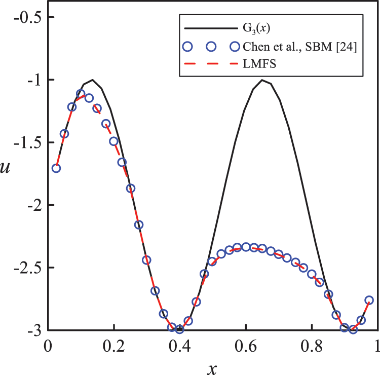
Figure 6: Numerical results of the shallow dam problem with G3(x)
A different number of boundary nodes N is used to show the convergence of the LMFS. Numerical results of the LMFS, the MFS [45], the BIE [46] and the SBM [24] are illustrated and compared in Table 1. From Table 1, it is not difficult to see that the LMFS can obtain the same numerical results with fewer boundary nodes than the other three methods.

Table 2 shows the number of iteration of the BPIM [47], the MFS [46] and the LMFS, and it is easy to see that the LMFS can achieve high accuracy with a smaller number of iterative steps compared with other methods.

The well-known electroplating problem [7,36,38] describes the painting process for coated metal surfaces. This problem plays a key role in the automobile manufacturing industry, especially in the application of anti-corrosion coating of automobile body. The principle of the painting process can be simply described as: a workpiece is immersed in the electrolyte paint containing charged ions; then the potential difference between the workpiece and the electrolytic cell is established; Finally, the paint particles are charged and deposited on the surface of the workpiece. The electroplating problem can be described as Signorini problems.
In this case, a Signorini problem of a square field (−0.5, 0.5)
where

Figure 7: The computational domain of the electropainting problem
Fig. 8 depicts the numerical results of the MFS [46], the BEM [26] and the LMFS of u on Γs when 80 boundary nodes and 400 interior notes are used. Different values of ε are considered, and the numerical results on Γs are presented with a curve of arc-length s (s = 0, s = 0.5, s = 1.5, s = 2) starts from corner point (0, 0) back to point (0, 0) in an anticlockwise direction. We can see from Fig. 8 that, the numerical results of the LMFS are very stable and fitting well with the results of other methods.


Figure 8: Numerical results with (a) ε = 0.4, (b) ε = 0.5, (c) ε = 0.55, (d) ε = 0.7
Fig. 9 shows the distribution of paint with different ε. The numerical results are obtained by using 80 boundary nodes. Figs. 8a and 9a indicate that the workpiece has been completely painted, and the amount of paint at the corner is the smallest. If ε increases, Figs. 8b–8c and Figs. 9b–9c denote that the paint film near the corner becomes thinner and eventually unpainted. When ε is increasing, Figs. 8d and 9d indicate that corner and vertex boundaries are not painted. Although there is no analytical solution, the results of the LMFS can be indirectly validated according to the reasonable physical characteristics. In addition, we can find that the LMFS obtain similar numerical results of the MFS [46,48], the BEM [26,41] and the SBM [24].
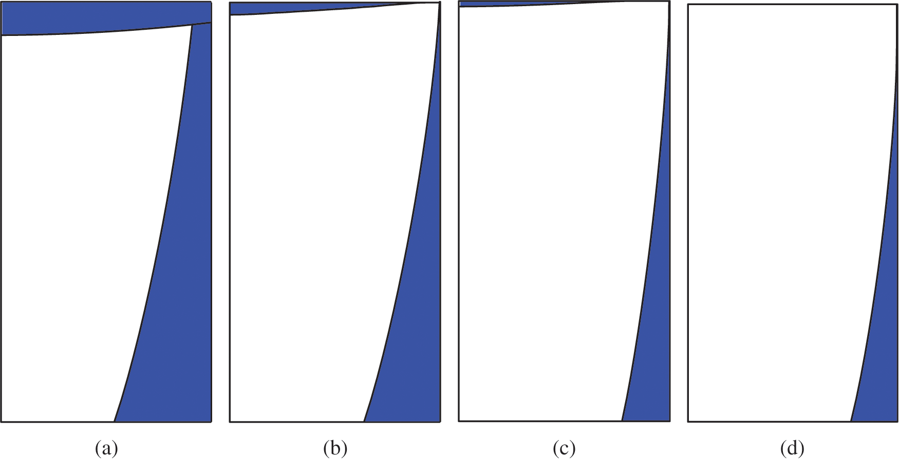
Figure 9: Paint distributions of (a) ε = 0.4, (b) ε = 0.5, (c) ε = 0.55, (d) ε = 0.7
As shown in Fig. 10a Signorini problem of a double-connected domain [15,24,36,48] is considered
where

Figure 10: A double-connected computational domain
We take N = 80 and Nin = 400 for the LMFS, and compare the numerical results obtained from the LMFS with the numerical results of the MFS [48] and the SBM [24] in Figs. 11 and 12, respectively. It is not difficult to see that the numerical results of the LMFS are in good agreement with numerical results of other two methods. This further indicates that the LMFS can deal with the Signorini problem of the double-connected domain very well.

Figure 11: Numerical u on Γs

Figure 12: Numerical q on Γs
In this paper, the LMFS is further applied to the Signorini problem. The stability of the LMFS is validated by considering several different numerical examples. The numerical results show that the number of source nodes and the initial value have little effect on the number of iterations steps. Comparing the numerical results obtained by LMFS with other methods, the LMFS can get more accurate results with the same number of nodes. The LMFS is more efficient, stable and has a higher convergence rate in dealing with Signorini problem. In our future work, more complicated problems, such as three-dimensional Signorini problems, Seepage problems, obstacle problems will be considered.
Funding Statement: The third author is supported by the National Science Foundation of China (No. 52109089). The fourth author is very thankful for the support of Post Doctor Program (2019M652281), Nature Science Foundation of Jiangxi Province (20192BAB216040).
Conflicts of Interest: The authors declare that they have no conflicts of interest to report regarding the present study.
1. Signorini, A. (1933). Sopra alune questioni di elastostatica. Atti della Societa Italiana per il Progresso delle Scienze, 21, 143–148. [Google Scholar]
2. Fichera, G. (1964). Problemi elastostatici con vincoli unilaterali: Il Problemi di Signorini con ambigue condizioni al contorno. Accademia nazionale dei Lincei, 8(7), 91–140. [Google Scholar]
3. Duvaut, G., Lions, J. (1972). Les inéquation en mécanique et en physique. Mathematics of Computation, 27. DOI 10.2307/2005636. [Google Scholar] [CrossRef]
4. Glowinski, R., Oden, J. T. (1985). Numerical methods for nonlinear variational problems. Journal of Applied Mechanics, 52(3), 739–740. DOI 10.1115/1.3169136. [Google Scholar] [CrossRef]
5. Maischak, M., Stephan, E. (2007). Adaptive hp-versions of boundary element methods for elastic contact problems. Computational Mechanics, 39(5), 597–607. DOI 10.1007/s00466-006-0109-y. [Google Scholar] [CrossRef]
6. Panzeca, T., Salerno, M., Terravecchia, S., Zito, L. (2008). The symmetric boundary element method for unilateral contact problems. Computer Methods in Applied Mechanics and Engineering, 197(33), 2667–2679. DOI 10.1016/j.cma.2007.03.026. [Google Scholar] [CrossRef]
7. Aitchison, J., Lacey, A., Shillor, M. (1984). A model for an electropaint process. IMA Journal of Applied Mathematics, 33(1), 17–31. DOI 10.1093/imamat/33.1.17. [Google Scholar] [CrossRef]
8. Poole, M. W., Aitchison, J. M. (1997). Numerical model of an electropaint process with applications to the automotive industry. IMA Journal of Management Mathematics, 8(4), 347–360. DOI 10.1093/imaman/8.4.347. [Google Scholar] [CrossRef]
9. Han, H., Guan, Z., Yu, C. (1988). The canonical boundary element analysis of a model for an electropaint process--The canonical boundary element approximation of a Signorini problem. Applied Mathematics, 3, 101–111. DOI 10.13299/j.cnki.amjcu.000153. [Google Scholar] [CrossRef]
10. Aitchison, J., Elliott, C., Ockendon, J. (1983). Percolation in gently sloping beaches. IMA Journal of Applied Mathematics, 30(3), 269–287. DOI 10.1093/imamat/30.3.269. [Google Scholar] [CrossRef]
11. Karageorghis, A. (1987). Numerical solution of a shallow dam problem by a boundary element method. Computer Methods in Applied Mechanics and Engineering, 61(3), 265–276. DOI 10.1016/0045-7825(87)90095-8. [Google Scholar] [CrossRef]
12. Poullikkas, A., Karageorghis, A., Georgiou, G. (1998). The method of fundamental solutions for Signorini problems. IMA Journal of Numerical, 18(1), 100–107. DOI 10.1093/imanum/18.2.273. [Google Scholar] [CrossRef]
13. Wang, L. H., Wang, G. H. (1999). A new mixed variational formulation for the contact problem in elasticity. Mathematica Numerica Sinica, 21(3), 237–244. DOI 10.3321/j.issn:0254-7791.1999.02.012. [Google Scholar] [CrossRef]
14. Han, H. (1991). A boundary element method for Signorini problems in three dimensions. Numerische Mathematik, 60(1), 63–75. DOI 10.1007/BF01385714. [Google Scholar] [CrossRef]
15. Spann, W. (1993). On the boundary element method for the Signorini problem of the Laplacian. Numerische Mathematik, 65(1), 337–356. DOI 10.1007/BF01385756. [Google Scholar] [CrossRef]
16. Costabel, M., Stephan, E. P. (1990). Coupling of finite and boundary element methods for an elastoplastic interface problem. SIAM Journal on Numerical Analysis, 27(5), 1212–1226. DOI 10.1137/0727070. [Google Scholar] [CrossRef]
17. Kupradze, V. D., Aleksidze, M. A. (1964). The method of functional equations for the approximate solution of certain boundary value problems. USSR Computational Mathematics and Mathematical Physics, 4(4), 82–126. DOI 10.1016/0041-5553(64)90006-0. [Google Scholar] [CrossRef]
18. Fan, C. M., Young, D. L., Chiu, C. L. (2009). Method of fundamental solutions with external source for the eigenfrequencies of waveguides. Journal of Marine Science and Technology, 17(3), 164–172. DOI 10.51400/2709-6998.1953. [Google Scholar] [CrossRef]
19. Hu, S., Fan, C. M., Chen, C. W., Young, D. L. (2005). Method of fundamental solutions for Stokes’ first and second problems. Journal of Mechanics, 21(1), 25–31. DOI 10.1017/S1727719100000514. [Google Scholar] [CrossRef]
20. Herrera, I. (2000). Trefftz method: A general theory. Numerical Methods for Partial Differential Equations, 16(6), 561–580. DOI 10.1002/(ISSN)1098-2426. [Google Scholar] [CrossRef]
21. Abou-Dina, M. S. (2002). Implementation of Trefftz method for the solution of some elliptic boundary value problems. Applied Mathematics and Computation, 127(1), 125–147. DOI 10.1016/S0096-3003(01)00063-7. [Google Scholar] [CrossRef]
22. Fang, H. M., Fan, C. M., Liu, Y. C., Hsiao, S. (2013). The least squares Trefftz method and the method of external source for the eigenfrequencies of waveguides. Journal of Marine Science and Technology, 21, 703–710. DOI 10.6119/JMST-013-0626-1. [Google Scholar] [CrossRef]
23. Chen, W., Tanaka, M. (2002). A meshless, integration-free, and boundary-only RBF technique. Computers & Mathematics with Applications, 43(3), 379–391. DOI 10.1016/S0898-1221(01)00293-0. [Google Scholar] [CrossRef]
24. Chen, B., Wei, X., Sun, L. L. (2020). The singular boundary method for solving Signorini problems. Engineering Analysis with Boundary Elements, 113(1), 306–314. DOI 10.1016/j.enganabound.2020.01.011. [Google Scholar] [CrossRef]
25. Li, J., Gu, Y., Qin, Q. H., Zhang, L. (2021). The rapid assessment for three-dimensional potential model of large-scale particle system by a modified multilevel fast multipole algorithm. Computers Mathematics with Applications, 89, 127–138. DOI 10.1016/j.camwa.2021.03.003. [Google Scholar] [CrossRef]
26. Zhang, S. G., Zhu, J. L. (2012). The boundary element-linear complementarity method for the Signorini problem. Engineering Analysis with Boundary Elements, 36(2), 112–117. DOI 10.1016/j.enganabound.2011.07.007. [Google Scholar] [CrossRef]
27. Kansa, E. J. (1990). Multiquadrics—A scattered data approximation scheme with applications to computational fluid-dynamics—I surface approximations and partial derivative estimates. Computers & Mathematics with Applications, 19(8–9), 127–145. DOI 10.1016/0898-1221(90)90270-T. [Google Scholar] [CrossRef]
28. Zheng, H., Yang, Z. J., Zhang, C. Z., Tyrer, M. (2018). A local radial basis function collocation method for band structure computation of phononic crystals with scatterers of arbitrary geometry. Applied Mathematical Modelling, 60(13), 447–459. DOI 10.1016/j.apm.2018.03.023. [Google Scholar] [CrossRef]
29. Qian, Z., Wang, L., Gu, Y. (2021). An efficient meshfree gradient smoothing collocation method (GSCM) using reproducing kernel approximation. Computer Methods in Applied Mechanics and Engineering, 374(3), 113573. DOI 10.1016/j.cma.2020.113573. [Google Scholar] [CrossRef]
30. Chen, J. S., Pan, C., Wu, C. T. (1996). Reproducing Kernel Particle Methods for large deformation analysis of non-linear structures. Computer Methods in Applied Mechanics and Engineering, 139(1–4), 195–227. DOI 10.1016/S0045-7825(96)01083-3. [Google Scholar] [CrossRef]
31. Zheng, H., Zhou, C. B., Yan, D. J., Wang, Y. S., Zhang, C. Z. (2020). A meshless collocation method for band structure simulation of nanoscale phononic crystals based on nonlocal elasticity theory. Journal of Computational Physics, 408(13), 109268. DOI 10.1016/j.jcp.2020.109268. [Google Scholar] [CrossRef]
32. Zheng, H., Zhang, C. Z., Wang, Y. S., Chen, W., Sladek, J. et al. (2017). A local RBF collocation method for band structure computations of 2D solid/fluid and fluid/solid phononic crystals. International Journal for Numerical Methods in Engineering, 110(5), 467–500. DOI 10.1002/nme.5366. [Google Scholar] [CrossRef]
33. Wu, C. P., Liu, Y. C. (2016). A review of semi-analytical numerical methods for laminated composite and multilayered functionally graded elastic/piezoelectric plates and shells. Composite Structures, 147, 1–15. DOI 10.1016/j.compstruct.2016.03.031. [Google Scholar] [CrossRef]
34. Li, J., Zhang, L., Qin, Q. H. (2021). A regularized method of moments for three-dimensional time-harmonic electromagnetic scattering. Applied Mathematics Letters, 112, 106746. DOI 10.1016/j.aml.2020.106746. [Google Scholar] [CrossRef]
35. Li, J., Zhang, L. (2021). High-precision calculation of electromagnetic scattering by the Burton-Miller type regularized method of moments. Engineering Analysis with Boundary Elements, 133(5), 177–184. DOI 10.1016/j.enganabound.2021.09.001. [Google Scholar] [CrossRef]
36. Zheng, H., Wu, M. X., Deng, C., Shi, Y. (2021). The local RBF collocation method for the 3D elastic tooth analysis. Applied Mathematical Modelling, 99(1), 41–56. DOI 10.1016/j.apm.2021.06.015. [Google Scholar] [CrossRef]
37. Xiong, J. G., Wen, J. C., Zheng, H. (2020). An improved local radial basis function collocation method based on the domain decomposition for composite wall. Engineering Analysis with Boundary Elements, 120(4), 246–252. DOI 10.1016/j.enganabound.2020.09.002. [Google Scholar] [CrossRef]
38. Liu, S., Li, P. W., Fan, C. M., Gu, Y. (2021). Localized method of fundamental solutions for two-and three-dimensional transient convection-diffusion-reaction equations. Engineering Analysis with Boundary Elements, 124(1), 237–244. DOI 10.1016/j.enganabound.2020.12.023. [Google Scholar] [CrossRef]
39. Gu, Y., Golub, M. V., Fan, C. M. (2021). Analysis of in-plane crack problems using the localized method of fundamental solutions. Engineering Fracture Mechanics, 256(5), 107994. DOI 10.1016/j.engfracmech.2021.107994. [Google Scholar] [CrossRef]
40. Xiong, J. G., Wen, J. C., Liu, Y. C. (2020). Localized boundary knot method for solving two-dimensional Laplace and bi-Harmonic equations. Mathematics, 8(8), 1218. DOI 10.3390/math8081218. [Google Scholar] [CrossRef]
41. Liu, Y. C., Fan, C. M., Yeih, W. C., Ku, C. Y., Chu, C. L. (2020). Numerical solutions of two-dimensional Laplace and biharmonic equations by the localized Trefftz method. Computers & Mathematics with Applications, 88, 120–134. DOI 10.1016/j.camwa.2020.09.023. [Google Scholar] [CrossRef]
42. Fischer, A. (1992). A special Newton-type optimization method. Optimization, 24(3–4), 269–284. DOI 10.1080/02331939208843795. [Google Scholar] [CrossRef]
43. Zhang, S., Zhu, J. (2013). A projection iterative algorithm boundary element method for the Signorini problem. Engineering Analysis with Boundary Elements, 37(1), 176–181. DOI 10.1016/j.enganabound.2012.08.010. [Google Scholar] [CrossRef]
44. Fan, C. M., Huang, Y. K., Chen, C. S., Kuo, S. R. (2019). Localized method of fundamental solutions for solving two-dimensional Laplace and biharmonic equations. Engineering Analysis with Boundary Elements, 101, 188–197. DOI 10.1016/j.enganabound.2018.11.008. [Google Scholar] [CrossRef]
45. Aitchison, J. M., Poole, M. W. (1998). A numerical algorithm for the solution of Signorini problems. Computational and Applied Mathematics, 94(1), 55–67. DOI 10.1016/S0377-0427(98)00030-2. [Google Scholar] [CrossRef]
46. Zheng, H. Y., Li, X. L. (2015). Application of the method of fundamental solutions to 2D and 3D Signorini problems. Engineering Analysis with Boundary Elements, 58(1), 48–57. DOI 10.1016/j.enganabound.2015.03.008. [Google Scholar] [CrossRef]
47. Ren, Y. L., Li, X. L. (2014). A Meshfree method for Signorini problems using boundary integral equations. Mathematical Problems in Engineering, 2014(5), 1–12. DOI 10.1155/2014/490127. [Google Scholar] [CrossRef]
48. Karageorghis, A., Lesnic, D., Marin, L. (2015). The method of fundamental solutions for solving direct and inverse Signorini problems. Computers & Structures, 151, 11–19. DOI 10.1016/j.compstruc.2015.01.002. [Google Scholar] [CrossRef]
 | This work is licensed under a Creative Commons Attribution 4.0 International License, which permits unrestricted use, distribution, and reproduction in any medium, provided the original work is properly cited. |