Computer Modeling in Engineering & Sciences

DOI: 10.32604/cmes.2022.016940

ARTICLE

Properties of Certain Subclasses of Analytic Functions Involving q-Poisson Distribution

Bilal Khan1,*, Zhi-Guo Liu1, Nazar Khan2, Aftab Hussain3, Nasir Khan4 and Muhammad Tahir2

1School of Mathematical Sciences and Shanghai Key Laboratory of PMMP, East China Normal University, Shanghai, 200241, China
2Department of Mathematics, Abbottabad University of Science and Technology, Abbottabad, 22010, Pakistan
3Department of Mathematics, King Abdulaziz University, Jeddah, 21589, Saudi Arabia
4Department of Mathematics, FATA University, Akhorwal (Darra Adam Khel), FR Kohat, 26000, Pakistan
*Corresponding Author: Bilal Khan. Email: bilalmaths789@gmail.com
Received: 12 April 2021; Accepted: 24 November 2021

1  Introduction, Basic Definitions and Motivation

A function f is said to be in the class A if the following normalization condition:

in the open unit disk:

is satisfied and having series representation:

Note that the notation C denote the set of all complex numbers. Also, let all those functions which are univalent in S are placed in functions class A.

Furthermore, let us consider a subclass T of the function class S, having the following series representation:

f(z)=z−∑k=2∞|ak|zk         (z∈U).(1)

Definition 1.1. [1] A function f is said to be in the class F(μ,ρ), if it satisfy the following inequality:

Definition 1.2. [1] A function f is said to be in the class H(μ,ρ), if it satisfy the following inequality:

It should be noted that for μ=0, we have

where F(ρ) and H(ρ) are the functions classes which were systematically studied by Silverman [2].

For a parameter ψ, if the values 0,1,2,3,⋯ with probabilities e−ψ,ψe−ψ1!,ψ2e−ψ2!,ψ3e−ψ3!⋯ are taken by a variable say N, then this variable N is said to have Poisson distribution. Thus

The Poisson distribution is a statistical distribution that calculates the probability of a certain number of events occurring in a particular time period. The Poisson distribution is commonly used to model rate of random events that occur (arrive) in some fixed time interval. The Poisson distribution models packet arrival times as an independent identically distributed process with an exponential distribution. However, it has been demonstrated in reality that packet inter-arrival durations do not follow an exponential distribution, resulting in a considerable increase in the error caused by modeling them as a Poisson distribution. User-initiated TCP (Transmission Control Protocol) session arrivals, such as remote login and file transfer, are well-modeled as Poisson processes with fixed hourly rates, but other connection arrivals deviate significantly from Poisson; modeling TELNET (Teletype Network Protocol) packet inter arrivals as exponential greatly underestimates the burstiness of TELNET traffic, according to studies.

The power series Υ(ψ,z) given by

Υ(ψ,z)=z+∑k=2∞ψk−1e−ψ(k−1)!zk          (∀z∈Uand  ψ>0) (2)

with its coefficients as probabilities of Poisson distribution which was introduced by Porwal [3] (see also [4–6]). The radius of convergence of Υ(ψ,z) is obviously infinity which can use proved by ratio test. Porwal [3] also defined and introduced the following series:

G(ψ,z)=2z−Υ(ψ,z)=z−∑k=2∞ψk−1e−ψ(k−1)!%zk      (∀z∈Uand  ψ>0). (3)

More about special functions and related topics, we may refer to [7–11].

The Basic (or q-) series and basic (or q-) polynomials, particularly basic (or q-) hypergeometric functions and basic (or q-) hypergeometric polynomials, are useful in a wide range of fields, including, for example, Non-Linear Electric Circuit Theory, Finite Vector Spaces, Combinatorial Analysis, Quantum Mechanics, Particle Physics, Mechanical Engineering, Lie Theory, Theory of Heat Conduction, Cosmology and Statistics (see for detail [12]).

In 1748 Euler studied a generating function for pn, the number of partitions of a positive integer n into positive integers by considering the infinite product.

which laid foundation of the study of basic hypergeometric series (also called q-hypergeometric series or q-series). Nevertheless it took a century to get the status of independent subject after the Heine’s conversion of a straightforward observation that

into a systematic theory of 2Φ1 basic hypergeometric series which is nothing but parallel to the theory of Gauss’ 2F1 hypergeometric series.

Beside from the influential study of Rogers and Thomae the subject stayed moderately comatose throughout the latter part of the nineteenth century up till Jackson embarked on a long lasting program of developing the theory of basic hypergeometric series in an organized mode (see [13] and [14]).

We next recollect certain elementary and useful concept details of the q-difference calculus, we let throughout the paper that

Definition 1.3. A q-generalization, q-extension, q-analogue or a q-deformation of an arbitrary number λ is given by

Definition 1.4. Let the q-factorial [n]q! with q∈(0,1) is define by

Definition 1.5. In a given subset of the set C of complex numbers, for function f∈A, the q-derivative (or q-difference) operator Dq is defined by (see [13] and [14])

(Dqf)(z)={f(z)−f(qz)(1−q)z(z≠0)f′(0)(z=0), (4)

provided that f′(0) exists.

In a given subset of C we can easily see from (4) that

whereas f is differentiable function. Furthermore, from (1) and (4) we obtain

(Dqf)(z)=1+∑k=2∞[k]qakzk−1. (5)

In Geometric Function Theory of Complex Analysis, the role of the q-difference (or the q-derivative) operator Dq is remarkably significant. In his article published by Ismail et al. (see [15]), presented the q-deformation of the class of S∗ of starlike functions. However, historically speaking, in 1989, in the context of Geometric Function Theory, the usage of the q-difference (or the q-derivative) operator Dq were systematically given by Srivastava [16].

More recently, Srivastava published a review article [12], in which the applications of the Dq operator in Geometric function Theory were survived. In the development of Geometric Function Theory, the works of Srivastava [16] and Ismail et al. [15] further motivate the researchers to give their finding to this field. For example, it were Wongsaijai et al. [17], who significantly studied certain subclasses of q-starlike functions. In particular, they studied the inclusion results, radius problems and certain sufficient conditions for their defined functions classes. More recently, the works of Wongsaijai et al. [17] have been generalized by Srivastava et al. (see [18,19]) in a systematic way. In fact Srivastava et al. (see [18,19]) make use of the q-Calculus and certain Janwoski functions in order to devolved their results, which essentially are the generalizations of [17]. Some more recent works related to q-calculus can be found in [20–28].

Motivated by the above-mentioned works of Srivastava [12,16] and Ismail et al. [15], in this article we shall mainly generalize the works presented in [1] and [3]. We shall study a number of sufficient conditions here. A necessary and sufficient condition shall be encounter for a certain function Gq(ψ,z)∈ Fq(μ,ρ) whose coefficients are nothing but merely the probabilities of q-Poisson distribution. In order to validate our results many new and known consequences are also included.

2  The Subclasses Fq(μ,ρ) and Hq(μ,ρ) of Analytic Functions

In this section, making use of the concept of q-calculus and the aforementioned works, we first define certain new subclasses Fq(μ,ρ) and Hq(μ,ρ) of analytic functions which involve the q-calculus. We then give certain sufficient conditions and closure results for these defined function classes. We have also highlighted some known and new consequences of our main results. The class Fq(μ,ρ) can be define as:

Definition 2.1. A function f with series representation (1) is to be placed in the class Fq(μ,ρ) if

Remark 1. First of all, it is easy to see that, if we put μ=0, we have

where TSq∗(ρ) is the function class, introduced and studied in [17]. Secondly, we have

where F(μ,ρ) is defined and studied in [1]. Thirdly, we see that

where TS∗(ρ) function class is defined and studied by Silverman [2].

Definition 2.2. A function f with series representation (1) is to be placed in the class Hq(μ,ρ) if

2.1 Sufficient Conditions for the Class Fq(μ,ρ) and Hq(μ,ρ)

Theorem 2.1. A function f of the form (1) is in the class Fq(μ,ρ) if and only if

∑k=2∞([k]q−μρ[k]q−ρ+μρ)|ak|≤(1−ρ). (6)

For the following function f1(z) the result is best possible

Proof. If we assume that f∈Fq(μ,ρ), then we have

ℜ(z(Dqf)(z)μz(Dqf)(z)+(1−μ)f(z))=ℜ(z−∑k=2[k]q|ak|zkz−∑k=2(μ[k%]q+(1−μ))|ak|zk%)≥ρ.

If the complex number z lie on the real axis side, then

is real. And so in limiting case if we take z→1−, along the real line, then, we have

We see that the last inequality is equivalent to (6).

Conversely, suppose that (6) hold true. Then adding

to both sides of (6), we get

(1−μ)∑k=2([k]q−1)|ak|≤(1−ρ)(1−∑k=2(μ[k]q+(1−μ))|ak|). (7)

On the other hand, we see that

|z(Dqf)(z)μz(Dqf)(z)+(1−μ)f(z)%−1|=|(1−μ)∑k=2([k%]q−1)|ak|zk−11−∑k=2(μ[k]q+(1−μ))|ak|zk−1|≤(1−μ)∑k=2([k]q−1)|ak|1−∑k=2(μ[k]q+(1−μ))|ak|. (8)

It is now easy to see from (7) that the last expression in (8) is bounded above by (1−ρ). Which evidently showing that f∈Fq(μ,ρ).

Corollary 1. If f∈Fq(μ,ρ) then, we have

Remark 2. First of all, we see that if we put μ=0, in Theorem 2.1, we get the known result due to Wongsaijai et al. (see [17]). Secondly if we put μ=0 and let q→1–, Theorem 2.1, we have the sufficient condition for the class S∗(ρ), which was studied by Silverman [2]. Thirdly, if we let q→1−, Theorem 2.1 coincide with a known result given in [1].

Theorem 2.2. A function f of the form (1) is in the class Hq(μ,ρ) if and only if

∑k=2∞[k]q([k]q−μρ[k]q−ρ+μρ)|ak|≤(1−ρ). (9)

The equality holds for the function f1(z) which is given by

Proof. This theorem can be proved by using the arguments similar which we used in Theorem 2.1.

2.2 Closure Theorems for the Class Fq(μ,ρ)

We define the function fϰ(z) (ϰ = 1,2,3,....,l) as

fϰ(z)=z−∑n=2∞|an,ϰ|zn          (z∈U).(10)

Furthermore, we now give certain closure results for the function involved in (10).

Theorem 2.3 Let the functions fϰ(z) (ϰ = 1,2,3,...,l) defined by (10) be in the class f∈Fq(μ,ρ). Then the function T∈Fq(μ,ρ), where

Proof. From (10), we have

Now making use of Theorem 2.1, we have

∑k=2∞([ k ]q−μρ[ k ]q−ρ+μρ)| ∑ϰ=1lΓϰak,ϰ |=∑ϰ=1lΓϰ(∑k=2∞([ k ]q−μρ[ k ]q−ρ+μρ)| ak,ϰ |)≤∑ϰ=1lΓϰ(1−ρ)=(1−ρ)           (∑ϰ=1lΓϰ=1).

Now by Theorem 2.1, the proof of Theorem 2.3 is completed.

Theorem 2.4. The class Fq(μ,ρ) defined in Definition 6 is closed under the convex combination.

Proof. To prove our result, we let that the given functions fϰ(z) (ϰ=1,2) which are defined by (10) be in the class Fq(μ,ρ). It is enough to show that

is in the class Fq(μ,ρ). Since

By Theorem 2.1, we have

which evidently complete the proof of Theorem 2.4.

3  The Classes Fq(μ,ρ) and Hq(μ,ρ) Involving q-Poisson Distribution

The Euler distribution or Heine distribution, as shown in [29] is a q-deformed Poisson distribution that is known in the literature. All of these, of course, are natural deformations in some sense, but they are all discrete. Kemp [30] demonstrated that the Euler and Heine distributions are, respectively, the limiting forms of a q-analogue of the negative binomial distribution and one of the binomial distribution. Jing [29] proposed a new type of q-analogue of the binomial distribution that uses the Euler distribution as its limiting form.

Furthermore, the theory of q-discrete distributions is quite significant because of theoretical probabilistic and statistical interest. In quantum probability it appears at Brownian motion, further from fascinating Markov chains with discrete finite or infinite state spaces it arises as a steady state distributions (see for example [29–31]). Our aim in this section is to consider a necessary and sufficient condition for a function Gq(ψ,z)∈ Fq(μ,ρ) such that its coefficients are probabilities of q-Poisson distribution. Some known consequences are also highlighted. The q-Poisson distribution P˙i

where

The graph of eqψ is given in Fig. 1.

In other words, if Nq takes the values 0,1,2,3,⋅⋅⋅ with probabilities eq−ψ,ψeq−ψ[1]!,ψ2eq−ψ[2]!,ψ3eq−ψ[3]!⋅⋅⋅  for the parameter ψ respectively, then Nq is called q-Poisson distributed.

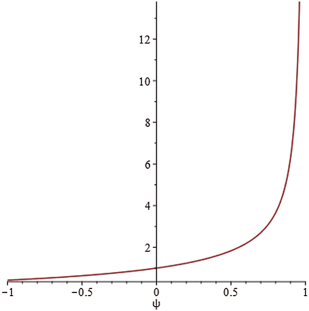
Figure 1: Graph of eqψ with q = 0.5 and −1<ψ<1

In the following equations we settled a power series so that its coefficients are probabilities the of q-Poisson distribution as

It could be seen that by ratio test the radius of convergence of Υq(ψ,z) is infinity. Therefore we define the following series:

Theorem 3.1. A function Gq(ψ,z) is to be placed in the functions class Fq(μ,ρ) if and only if

q(1−ρμ)ψeqψ<(1−ρ)             (ψ>0). (11)

Proof. Since

According to Theorem 2.1, we must show that

Therefore, we now consider

∑k=2∞([k]q−μρ[k]q−ρ+μρ)(ψk−1[k−1]q!eq−ψ)=eq−ψ∑k=2∞(([k]q−1)(1−μρ)+(1−ρ))(ψk−1[k−1]q!)=eq−ψ(q(1−μρ)∑k=2∞[k−1]qψk−1[k−1]q!+(1−ρ)∑k=2∞(ψk−1[k−1]q!))=eq−ψ(q(1−μρ)∑k=2∞ψk−1[k−2]q!)+eq−ψ(1−ρ)∑k=1∞(ψk[k]q!)=eq−ψ(q(1−μρ)ψ∑k=0∞ψk[k]q!)+eq−ψ(1−ρ)∑k=1∞(ψk[k]q!)=eq−ψ(q(1−μρ)ψeqψ+(1−ρ)(eqψ−1)). (12)

The last expression in (12) is evidently bounded by functional (1−ρ) in the case if and only if relation given in (11) holds true.

Thus we complete the required proof of our Theorem.

Corollary 2. A function Gq(ψ,z) is to be placed in the functions class Fq(0,ρ)=TSq∗(ρ) if and only if

qψeqψ<(1−ρ)             (ψ>0). (13)

Remark 3. If we set q→1− in Theorem 3.1, it will lead us to the result given by Porwal [3].

Theorem 3.2. A function Gq(ψ,z) is to be placed in the class Fq(μ,ρ) if and only if

q(1−ρμ)ψeqψ<(1−ρ)             (ψ>0). (14)

Proof. Since

According to Theorem 2.2, we must show that

Therefore, we now consider

∑k=2∞[k]q([k]q−μρ[k]q−ρ+μρ)(ψk−1[k−1]q!eq−ψ)=∑k=2∞{([k]q−1)([k]q−2)(1−μρ)+(3−μρ−ρ)([k]q−1)+(1−ρ)}(ψk−1[k−1]q!eq−ψ)=eq−ψ(q3(1−μρ)∑k=3∞ψk−1[k−3]q!+(2−qμρ−ρ+q)q⋅∑k=2∞ψk−1[k−2]q!%+(1−ρ)∑k=2∞ψk−1[k−1]q!)=eq−ψ(q3ψ2(1−μρ)eqψ+(2−qμρ−ρ+q)qψeqψ+(1−ρ)(eqψ−1))=q3ψ2(1−μρ)+(2−qμρ−ρ+q)qψ+(1−ρ)(1−eq−ψ). (15)

We in last expression see that the (1−ρ) is bound of (15) if and only if (11) holds true.

Thus we have completed the proof of our Theorem.

Remark 4. If in Theorem 3.2, we let q→1−, we will arrive at the result given by Porwal [3].

4  Concluding Remarks and Observations

In our present work, by using the q-calculus, we have first defined certain new subclasses of an analytic function. We then gave necessary and sufficient conditions for each of the defined function classes. We have also studied necessary and sufficient conditions for a function whose coefficients are probabilities of q-Poisson distribution. We have also given particular known and new consequences in the form of Remarks and Corollaries.

The usage of basic (or q-) series in many diverse areas of Mathematics and Physics makes it very important. By using the basic (or q-) series, some wonderful works have been done. As we described in Section 1, the Srivastava’s observation [12] about the so-called (p, q)-calculus, we arrived at the point that indeed the result presented in this paper can be produced for the rather straightforward (p, q)-variations.

Authors’ Contributions: All authors contributed equally to this work. All authors have read and agreed to the published version of the manuscript.

Availability of Data and Materials: Not applicable.

Funding Statement: The authors received no specific funding for this study.

Conflicts of Interest: The authors declare that they have no conflicts of interest to report regarding the present study.

References

 1.  Altintas, O., Owa, S. (1988). On subclasses of univalent functions with negative coefficients. Pusan Kyongnam Mathematical Journal, 4, 41–56. DOI JAKO198810736820756. [Google Scholar]

 2.  Silverman, H. (1975). Univalent functions with negative coefficients. Proceedings of the American Mathematical Society, 51(1), 109–116. DOI 10.1090/S0002-9939-1975-0369678-0. [Google Scholar] [CrossRef]

 3.  Porwal, S. (2014). An application of a poisson distribution series on certain analytic functions. Journal of Complex Analysis, 2014, 1–3. DOI 10.1155/2014/984135. [Google Scholar] [CrossRef]

 4.  Murugusundaramoorthy, G. (2018). Univalent functions with positive coefficients involving poisson distribution series. Honam Mathematical Journal, 40(3), 529–538. DOI JAKO201831342439007. [Google Scholar]

 5.  Murugusundaramoorthy, G. (2018). Subclasses of starlike and convex functions involving poisson distribution series. Afrika Matematika, 28(7), 1357–1366. DOI 10.1007/s13370-017-0520-x. [Google Scholar] [CrossRef]

 6.  Murugusundaramoorthy, G., Vijaya, K., Porwal, S. (2016). Some inclusion results of certain subclass of analytic functions associated with poisson distribution series. Hacettepe Journal of Mathematics and Statistics, 45(4), 1101–1107. DOI 10.15672/HJMS.20164513110. [Google Scholar] [CrossRef]

 7.  Attiya, A. A., Lashin, A. M., Ali, E., Agarwal, P. (2021). Coefficient bounds for certain classes of analytic functions associated with faber polynomial. Symmetry, 13(2), 1–23. DOI 10.3390/sym13020302. [Google Scholar] [CrossRef]

 8.  Morales-Delgado, V. F., Gomez-Aguilar, J. F., Saad, K. M., Khan, M. A., Agarwal, P. (2019). Analytic solution for oxygen diffusion from capillary to tissues involving external force effects: A fractional calculus approach. Physica A: Statistical Mechanics and its Applications, 523, 48–65. [Google Scholar]

 9.  Yassen, M. F., Attiya, A. A., Agarwal, P. (2020). Subordination and superordination properties for certain family of analytic functions associated with Mittag–Leffler function. Symmetry, 12(10), 1724. [Google Scholar]

10. Salahshour, S., Ahmadian, A., Senu, N., Baleanu, D., Agarwal, P. (2015). On analytical solutions of the fractional differential equation with uncertainty: Application to the basset problem. Entropy, 17(2), 885–902. DOI 10.3390/e17020885. [Google Scholar] [CrossRef]

11. Zhou, S. S., Areshi, M., Agarwal, P., Shah, N. A., Chung, J. D. et al. (2021). Analytical analysis of fractional-order multi–dimensional dispersive partial differential equations. Symmetry, 13(6), 1–13. DOI 10.3390/sym13060939. [Google Scholar] [CrossRef]

12. Srivastava, H. M. (2020). Operators of basic (or q-) calculus and fractional q-calculus and their applications in geometric function theory of complex analysis. Iranian Journal of Science and Technology, Transactions A, 44(1), 327–344. DOI 10.1007/s40995-019-00815-0. [Google Scholar] [CrossRef]

13. Jackson, F. H. (1910). On q-definite integrals. Pure and Applied Mathematics Quarterly, 41, 193–203. [Google Scholar]

14. Jackson, F. H. (1910). q-difference equations. American Journal of Mathematics, 32(4), 305–314. DOI 10.2307/2370183. [Google Scholar] [CrossRef]

15. Ismail, M. E. H., Merkes, E., Styer, D. (1990). A generalization of starlike functions. Complex Variables: Theories and Applications, 14(1–4), 77–84. DOI 10.1080/17476939008814407. [Google Scholar] [CrossRef]

16. Srivastava, H. M. (1989). Univalent functions, fractional calculus, and associated generalized hypergeometric functions. In: Srivastava, H. M., Owa, S. (Eds.Univalent functions, fractional calculus, and their applications, pp. 329–354. New York, Chichester, Brisbane and Toronto: Halsted Press (Ellis Horwood Limited, ChichesterJohn Wiley and Sons. [Google Scholar]

17. Wongsaijai, B., Sukantamala, N. (2016). Certain properties of some families of generalized starlike functions with respect to q-calculus. Abstract and Applied Analysis, 2016, 1–8. DOI 10.1155/2016/6180140. [Google Scholar] [CrossRef]

18. Srivastava, H. M., Tahir, M., Khan, B., Ahmad, Q. Z., Khan, N. (2019). Some general classes of q-starlike functions associated with the Janowski functions. Symmetry, 11(2), 1–14. DOI 10.3390/sym11020292. [Google Scholar] [CrossRef]

19. Srivastava, H. M., Tahir, M., Khan, B., Ahmad, Q. Z., Khan, N. (2019). Some general families of q-starlike functions associated with the Janowski functions. Filomat, 33(9), 2613–2626. DOI 10.2298/FIL1909613S. [Google Scholar] [CrossRef]

20. Ibrahim, R. W. (2020). Geometric process solving a class of analytic functions using q-convolution differential operator. Journal of Taibah University for Science, 14(1), 670–677. DOI 10.1080/16583655.2020.1769262. [Google Scholar] [CrossRef]

21. Ibrahim, R. W., Elobaid, R. M., Obaiys, S. J. (2021). On subclasses of analytic functions based on a quantum symmetric conformable differential operator with application. Advances in Difference Equations, 2020(1), 1–14. DOI 10.1186/s13662-020-02788-6. [Google Scholar] [CrossRef]

22. Ibrahim, R. W., Elobaid, R. M., Obaiys, S. J. (2020). A class of quantum Briot–Bouquet differential equations with complex coefficients. Mathematics, 8(5), 1–13. DOI 10.3390/math8050794. [Google Scholar] [CrossRef]

23. Ibrahim, R. W., Elobaid, R. M., Obaiys, S. J. (2020). Geometric inequalities via a symmetric differential operator defined by quantum calculus in the open unit disk. Journal of Function Spaces, 2020, 8. DOI 10.1155/2020/6932739. [Google Scholar] [CrossRef]

24. Ibrahim, R. W., Hadid, S. B., Momani, S. (2020). Generalized Briot–Bouquet differential equation by a quantum difference operator in a complex domain. International Journal of Dynamics and Control, 8(3), 762–771. DOI 10.1007/s40435-020-00616-z. [Google Scholar] [CrossRef]

25. Khan, B., Liu, Z. G., Srivastava, H. M., Khan, N., Darus, M. et al. (2020). A study of some families of multivalent q-starlike functions involving higher-order q-derivatives. Mathematics, 8(9), 1–12. DOI 10.3390/math8091470. [Google Scholar] [CrossRef]

26. Khan, B., Srivastava, H. M., Khan, N., Darus, M., Ahmad, Q. Z. et al. (2021). Applications of certain conic domains to a subclass of q-starlike functions associated with the Janowski functions. Symmetry, 13(4), Article ID 574, 1–18. DOI 10.3390/sym13040574. [Google Scholar] [CrossRef]

27. Liu, Z. G. (2003). Some operator identities and q-series transformation formulas. Discrete Mathematics, 265(1–3), 119–139. DOI 10.1016/S0012-365X(02)00626-X. [Google Scholar] [CrossRef]

28. Liu, Z. G. (2002). An expansion formula for q-series and applications. The Ramanujan Journal, 6(4), 429–447. DOI 10.1023/A:1021306016666. [Google Scholar] [CrossRef]

29. Jing, S. (1994). The q-deformed binomial distribution and its asymptotic behaviour. Journal of Physics A: Mathematical and General, 27(2), 493–499. DOI 10.1088/0305-4470/27/2/031/meta. [Google Scholar] [CrossRef]

30. Kemp, A. W. (2002). Certain q-analogue of the binomial distribution. Sankhyā The Indian Journal of Statistics, Series A, 64, 293–305. DOI /stable/25051397. [Google Scholar]

31. Saitoh, A., Yoshida, H. (2000). A q-deformed poisson distribution based on orthogonal polynomials. Journal of Physics A: Mathematical and General, 33(7), 1435–1444. DOI 10.1088/0305-4470/33/7/311/meta. [Google Scholar] [CrossRef]

32. Kupershmidt, B. A. (2000). q-probability: I. Basic discrete distributions. Journal of Nonlinear Mathematical Physics, 7(1), 73–93. DOI 10.2991/jnmp.2000.7.1.6. [Google Scholar] [CrossRef]

This work is licensed under a Creative Commons Attribution 4.0 International License, which permits unrestricted use, distribution, and reproduction in any medium, provided the original work is properly cited.