Computer Modeling in Engineering & Sciences

DOI: 10.32604/cmes.2022.018879

ARTICLE

A Numerical Modelling Method of Fractured Reservoirs with Embedded Meshes and Topological Fracture Projection Configurations

Xiang Rao1,2,* and Yina Liu1,2

1Cooperative Innovation Center of Unconventional Oil and Gas (Ministry of Education & Hubei Province), Yangtze University, Wuhan, China
2School of Petroleum Engineering, Yangtze University, Wuhan, China
*Corresponding Author: Xiang Rao. Emails: raoxiang0103@163.com; raoxiang@yangtzeu.edu.cn
Received: 22 August 2021; Accepted: 01 December 2021

1  Introduction

Accurate and efficient numerical simulation of flow in fractured media is a challenging and important topic, which is of great interest in hydrocarbon recovery [1–4], aquifer management, and carbon dioxide geological sequestration, etc. The discrete fracture model (DFM), which explicitly handles large-scale fractures, has been a common technique to numerically model the flow in fractured media over the past two decades. Unstructured matrix meshes were generated to conform to the geometry of complex fracture network such that fractures lied at the interfaces between matrix cells. DFM thus accurately accounted for the effect of complex fracture geometries on flow, yielding physical and accurate simulation results. For single-phase flow, multiphase flow, and compositional flow models, A large variety of DFMs with different based numerical calculation methods had been presented in literature for single-phase flow, multiphase flow, and compositional flow models, including finite difference method (FDM) [5,6], Galerkin finite element method (FEM) [6,7], finite volume method (FVM) [7], control volume finite element method (cvFEM) [8,9], and mixed finite element method (mFEM) [10]. However, a high-quality unstructured mesh to match complex fracture networks was challenging to generate [11], and often comprised of huge numbers of small-size cells near fractures. These resulted in high computing costs, limiting the field applications of DFM.

The above problems led to the emergence of embedded discrete fracture model (EDFM) which made use of non-conforming mesh. Li et al. [12] proposed EDFM, in which fractures were treated as source or sink terms in matrix cells, allowing for the use of a structured background mesh. Then, inter-cell connections were obtained by figuring out the geometric relationships between embedded discrete fractures and structured matrix cells. That is, in contrast to DFM, EDFM avoided the complexity of creating a high-quality conforming mesh. EDFM has been used to numerically simulate a variety of flow problems in fractured media [13–21]. To increase computational performance in heterogeneous formations, Hajibeygi et al. [22] presented a hierarchical embedded fracture model utilizing iterative multiscale FVM. Moinfar et al. [23] developed an efficient EDFM for three-dimensional (3D) compositional reservoir simulation. Mimetic FDM and its multiscale technique-based EDFM were reported by Yan et al. [24] and Zhang et al. [25], respectively, in which velocity and phase pressure fields were solved simultaneously. Zeng et al. [26] presented a coupled model of EDFM and extended finite element method (XFEM) to study dynamic behaviors of hydraulic fractures. Rao et al. [27] presented a multi-layer virtual-cell EDFM to improve the early-time simulation accuracy for the production forecast of fractured horizontal wells. Wu et al. [28] proposed a Green element method-based EDFM that may yield high-accuracy results for single-phase flow.

Although EDFM had been validated by the above works and used in various porous flow problems [29,30], Tene et al. [31] found that classical EDFM could not effectively handle cases when fracture permeability was lower than matrix permeability, especially when flow barriers were present. To resolve the limitation, they developed a projection-based EDFM (pEDFM) by projecting the fracture cells to matrix-cell interfaces, constructing additional fracture-matrix (f-m) connections while weakening the original matrix-matrix (m-m) connections. Jiang et al. [32] pointed out that large errors could be induced for EDFM to handle multiphase flow across fractures, and presented an improved pEDFM to effectively resolve the limitation. Rao et al. [33] developed a modified pEDFM that included a practical approach for determining fracture cell projection configuration and new fracture-fracture (f-f) connections to make the model framework more complete. Liu et al. [34] used pEDFM to model carbon dioxide geological sequestration in depleted complex-shape shale reservoirs. Wang et al. [35] presented a 3D pEDFM for compositional simulation of fractured reservoirs. Ren et al. [36,37] coupled pEDFM and XFEM to study flow in fractured reservoirs by considering geomechanics. Rao et al. [38] constructed a pEDFM based two-phase flow heat and mass transfer model, and found that pEDFM could eliminate the computational errors of temperature profiles in EDFM. These works indicated that, pEDFM had a better generalization of flow models than EDFM, and a lower computational cost than DFM. That is to say, pEDFM possessed the advantages of both DFM and EDFM, and hence deserved more attention.

However, this work points out that, in most cases, pEDFM still cannot effectively handle embedded flow barriers, implying that Tene et al. [31] had not completely accomplished their initial goal. By analysing the essence of pEDFM, this paper presents and proves an equivalence theorem that shows that the projection configuration of a fracture being physical is equivalent to it being topologically homeomorphic to fracture. Based on the equivalence theorem, pEDFM can yield physical results for flow barriers. Then, we present a practical method to handle complex geological conditions of reservoir model with a 3D Cartesian grid.

2  A Brief Review of pEDFM

2.1 Governing Equations

Take the immiscible multiphase flow problem as an example to illustrate the governing equations. For phase a, the mass conservation equation is written as

∇⋅(kkraBaμa∇pa)+q~a,well=∂∂t(ϕsaBa)(1)

where k is the absolute permeability; kra, Ba, μa, pa, sa are relative permeability, volume factor, viscosity, the converted pressure by considering gravity and saturation of phase a; q~a,well is the flow term of phase a for wells (source or sink term);

The discrete form of Eq. (1) is always obtained by block-center finite volume method. For the ith cell, it is written in Eq. (2).

∑j=1nqijt+Δt+qa,well,it+Δt=ViΔt[(ϕsa,iBa,i)t+Δt−(ϕsa,iBa,i)t](2)

where qa,well,i=∫Ωq~a,welldV, Ω is the computational domain.

The flux across the interface of two connected cells is approximated by two-point linear flux approximation, that is Eq. (3).

qijt+Δt=−Tijλa,ijt+Δt(pa,it+Δt−pa,jt+Δt)(3)

where Tij and λa,ij are the transmissibility and phase mobility of the connection. Tij is the half of the harmonic mean of two half-transmissibilities, that is Eq. (4).

Tij=TiTjTi+Tj(4)

λa,ij is expressed as Eq. (5).

λa,ij=kra,ijμa,ijBa,ij(5)

The upstream and arithmetic average schemes are used for the terms (relative permeability) subject to the saturation and the terms (viscosity and volume factor) subject to pressure, respectively, these are in Eq. (6).

μa,ij=μa,i+μa,j2,Ba,ij=Ba,i+Ba,j2,kra,ij={kra,iif pa,i≥pa,jkra,jif pa,i<pa,j(6)

As a result, the ultimate discrete scheme of Eq. (1) is expressed as Eq. (7).

∑j=1n{−Tijλa,ij(pa,i−pa,j)}t+qa,well,i=ViΔt[(ϕsa,iBa,i)t+Δt−(ϕsa,iBa,i)t](7)

2.2 pEDFM Framework

Tene et al. [31] presented pEDFM as a way to expand traditional EDFM to efficiently treat fractures with a wide variety of permeabilities (i.e., from flow barriers to highly conductive fractures). Jiang et al. [32] pointed out large errors will be induced for EDFM to handle multiphase flow across fractures, and presented an improved pEDFM to resolve the limitation. These studies revealed that pEDFM had higher physical model generalization than traditional EDFM, indicating that this new model required more attention.

Firstly, the basic ideas of pEDFM are briefly introduced below. As shown in Fig. 1, pEDFM, like EDFM, divides the reservoir calculation domain using a structured or orthogonal mesh (recorded as background matrix mesh) and embeds fractures into the background mesh to create fracture cells divided by intersecting lines (surfaces) between matrix cells. In reservoir simulation, the reservoir boundary condition is always assumed to be closed. The essential difference between pEDFM and EDFM lies in the different connections between cells.

Figure 1: Sketch of neighboring matrix cells, a contained fracture cell and its projections on interfaces

As shown in Fig. 1, the grey squares represent three matrix cells mi, mj and mk, respectively. The yellow segment denotes a fracture cell f in mi. Two red segments represent the x-direction projection of f on interface Γij (denoted by fx) and y-direction projection of f on interface Γik (denoted by fy), respectively.

2.2.1 Construction of Additional f-m Connections

For these three matrix cells and a fracture cell, there is only one fracture-matrix (f-m) connection in classical EDFM, i.e., f-mi. However, additional f-m connections f-mj and f-mk are constructed in pEDFM, and the areas of fx and fy are considered as the flow areas of f-mj and f-mk connections, respectively. Besides, the original f-mi connection needs to be weakened.

In pEDFM, for f-mi connection, the ‘matrix half’ and ‘fracture half’ transmissibilities are given as Eq. (8).

Tmi=kmiAf⟨d⟩fmi,Tf=kfAfwf(8)

where kmi and kf are the permeabilities of mi and f, respectively, wf is the aperture of f. Af is the area of f, ⟨d⟩fmi is the average normal distance between f and mi, which is generally approximated by assuming that phase pressure within a matrix cell distributes linearly along the direction normal to the contained fracture cell, that is Eq. (9).

⟨d⟩fmi=∫mi|n→⋅r→|dVVmi(9)

For added f-m connections, the areas of fx and fy are used to determine the transmissibilities of these connections, by taking f-mj connection as an example, the ‘matrix half’ and ‘fracture half’ transmissibilities are given as Eq. (10).

Tmj=kmjAfxdfmj,Tf=kfAfwf(10)

where kmj is the permeability of mj, Afx denotes the area of fx, dfmj is the distance between the centers of mj and f.

Then Tfmj is calculated as Eq. (11).

Tfmj=(Tmj−1+Tf−1)−1(11)

However, assuming that there is fluid flowing from mj to f, the physical flowing route is mj-mi-f, so Jiang et al. [32] discussed that the transmissibility Tfmj should take the effect of mi (i.e., Tmi) into account, which is Eq. (12).

Tfmj=(Tmj−1+Tmi−1+Tf−1)−1(12)

Similarly, the transmissibility of the f-mk connection can be obtained in Eq. (13).

Tfmk=(Tmk−1+Tmi−1+Tf−1)−1,Tmk=kmkAfydfmk(13)

where kmk is the permeability of mk, Afx denotes the area of fx, dfmk is the distance between the centers of mk and f.

2.2.2 Weakening of m-m Connections

Because the flow areas of m-m connections are blocked by additional f-m connections, the transmissibility of corresponding m-m connections should be weakened. Take mi-mj connection as an example, the effective flow area of mi-mj connection is equal to the area of Γij minus the area of fx, so the half-transmissibility Ti and Tj for Tmimj are given as Eq. (14).

Ti=kmi(Aij−Afx)di,Tj=kmj(Aij−Afx)dj(14)

where Aij is the area of Γij, di is the distance from the center of mi to Γij, dj is the distance from the center of mj to Γij.

2.3 Determination of Projection Configuration of Fracture Cells

In the original paper by Tene et al. [31], there was no obvious statement about the determination criteria of the projection configuration of fracture cells, but it indicated that in each direction we should select the interface that is closest to the fracture-cell center, and this implicit criterion is simply denoted as the “smaller distance criterion”. Jiang et al. [32] pointed out that, smaller distance criterion may give an unphysical fracture-cell projection configuration in some cases when the distances between the fracture-cell center and two neighboring interfaces are the same in at least one direction. To resolve this problem, they presented an additional criterion that the intersections between the fracture-cell projections and the fracture cell should not be on the same side of the fracture-cell center, which is simply denoted as the “different side criterion”. Based on these two criteria, Rao et al. [33] presented a practical method namely the ‘micro-translation method’ to efficiently select the projected interfaces of fracture cells to determine the fracture-cell projection configurations.

3  Not-Fully-Achieved Motivation

The motivation of the original pEDFM proposed by Tene et al. [31] is to modify EDFM to effectively handle cases when fracture permeability is lower than matrix permeability, especially those cases with flow barriers.

However, it is found that pEDFM still fails when dealing with flow barriers in most cases, that is, it can not accurately characterize the block effect of flow barriers. As shown in Fig. 2, a flow barrier (plotted in yellow) is divided into three cells f1, f2, and f3 by matrix cells m1, m2 and m3. By following smaller distance and different sides criteria, obtained fracture-cell projection configurations are plotted in Fig. 3, in which red segments, blue segments and green segments denote projection configurations of f1, f2 and f3, respectively. A1, A2 and A3 denote areas of x-direction projections of f1, f2 and f3, respectively. The total projection areas on interfaces Γ12 and Γ23 can be calculated as Eq. (15).

A12p=A1+A2,A23p=A2(15)

Figure 2: Schematics of an example in which pEDFM fails to handle the flow barrier

Figure 3: Schematics of the fracture-cell projection configurations of the given example

Then, by following Eq. (7), the ‘matrix half’ transmissibilities for the m1-m2 connection are Eqs. (16) and (17).

T1=km1(A12−A12p)d1=km1(A12−A1−A2)d1>0(16)

T2=km2(A12−A12p)d2=km2(A12−A1−A2)d2>0(17)

Consequently, the transmissibility of the m1-m2 connection is calculated as Eq. (18).

T12=(T1x−1+T2x−1)−1>0(18)

Similarly, the transmissibility of the m2-m3 connection is obtained as Eq. (19).

T23>0(19)

In Fig. 4, the blue arrows denote the connections whose transmissibility is not 0. Imagining that there is fluid flowing into matrix cell m1 along the positive direction of x-axis, the fluid can still pass through the flow barrier along the path “l-m1-m2-m3-r”, which is unphysical, meaning the flow barrier is not effectively handled.

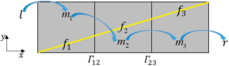
Figure 4: Schematics of the route along which fluid flow across the flow barrier

Fig. 5 depicts another example. A flow barrier is divided into four cells f1, f2, f3 and f4 by matrix cells m1, m2, m3 and m4. According to the same analysis as the previous example, fluid can still flow across the flow barrier along the route “l-m1-m2-m3-m4-r”, which is also unphysical. Furthermore, we give an example in Fig. 6 to validate the above analysis. As is shown, a flow barrier whose geometry is the same as that in Fig. 5 is embedded in the 60 m × 60 m reservoir model, and a water injection well and a producer are at position (10, 30) and position (50, 30), respectively. The initial pressure is 20 MPa, and the constant injection rate is 1m3/d, and the constant BHP of the producer is 10 MPa. Fig. 6 shows the water saturation profiles with different mesh sizes at the 300th day from the original pEDFM, which illustrates the unphysical computational results that injected water flow across the flow barrier and the unphysical results are independent of the mesh size. Moreover, it can be predicted similarly that when the number of matrix cells in a row continues to increase in Fig. 5, the result will still be unphysical, which shows that, in most cases pEDFM cannot effectively handle the flow barrier, implying that Tene et al. [31] have not fully achieved their original motivation.

Figure 5: Schematics of the route along which fluid flow across the flow barrier when the matrix-cell number increases to 4

Figure 6: Water saturation profiles with different mesh sizes (a) 5 m (b) 4 m (c) 2 m (d) 1 m

4  What is Physical Projection Configuration?

The issue of selecting a physical projection configuration was first noticed by Jiang et al. [32]. They pointed out that in some special cases, unphysical projection configurations may be implemented by only following the “smaller distance criterion”. For an example shown in Fig. 7, a fracture cell is located on the diagonal of a rectangular matrix cell, and the fracture-cell center coincides with the matrix-cell center. By following the “smaller distance criterion”, edge 2 or edge 4 can be selected in x-direction, and edge 1 or edge 3 can be selected in y-direction, resulting in four projection configurations (i.e., edges 2-1, edges 2-3, edges 4-1, edges 4-3). However, Jiang et al. [32] pointed out that the projection configurations of edges 1-4 and edges 2-3 do not conform to the actual effect of fracture geometry orientation on flow and thus are unphysical. To resolve this limitation, Jiang et al. proposed the different sides criterion to avoid those unphysical projection configurations.

Figure 7: The example given by Jiang et al.

However, the examples in Section 3 show that “smaller distance” and “different sides” criteria are insufficient to obtain physical projection configurations. Moreover, it can be seen that these two criteria are subjective and lack rigorous analysis. Therefore, a profound and rigorous analysis of “physical fracture-projection configuration” is required, as well as clarification of its geometric nature.

4.1 Introduction of the Equivalence Theorem

In this paper, it will be pointed out that determining physical projection configuration is the most crucial step of pEDFM. In addition, when determining the physical projection configuration, it should focus on an entire fracture, not a single fracture cell. It should be noted that a fracture cell that does not penetrate the entire matrix cell (as shown in Fig. 8) cannot completely block the flow across the matrix cell, so the “shortest distance” and “different sides” criterion can be directly applied to determine the projection configuration of the fracture cell. Therefore, unless otherwise noted, the fractures mentioned below are those removing fracture cells at both ends that do not penetrate the whole matrix cell.

Figure 8: Schematics of those fracture cells which are not penetrating the matrix cell

In this paper, a necessary and sufficient condition is given to judge whether the projection configuration of a fracture is physical, that is, the equivalent geometric description of “projection configuration of a fracture is physical”, and is simply denoted as “equivalence theorem” in the following,

Equivalence theorem: the projection configuration of a fracture (regardless of the fracture cells which are at both ends of the fracture and do not penetrate the entire matrix cell) being physical is equivalent to it being topologically homeomorphic to the fracture. That is, from the geometric view, the topological properties of the projection configuration are the same as those of the fracture.

The conception of homeomorphism in topology is used in the statement of the above theorem. The following is a quick description of the conception, and detailed explanations can be found in the textbook [39].

In topology, two topological spaces {X, TX} and {Y, TY} are called homeomorphic when a map f : X Y satisfies the following conditions: (i) f is bijection; (ii) f is continuous; (iii) the inverse of f is continuous.

Then f is called the homeomorphism between {X, TX} and {Y, TY}, and {X, TX} and {Y, TY} have the same topological properties.

Colloquially, topological space is a geometric object, and homeomorphism is to extend and continuously bend the object to make it a new object. So a square and a circle are homeomorphic, but a sphere and a torus are not.

To prove the equivalence theorem, this paper firstly studies the essence of pEDFM, and then obtains a lemma to prove the theorem.

4.2 Analysis of the Essence of pEDFM

EDFM handles fracture cells as the source or sink terms in matrix cells, whereas DFM uses unstructured matrix cells to match fractures, resulting in fractures being located on the matrix cell interfaces. Due to the two distinct fracture treatments, these two models exhibit distinct characteristics: (i) Because EDFM does not require a high-quality unstructured mesh to match the fracture geometry, it can be applied only to the physical models in which fractures are the source or sink terms of matrix cells (e.g., production or injection simulation of a multi-stage fractured horizontal well), EDFM has significant limitations in the generality of physical models; (ii) DFM has good generalization of physical models, but it is difficult to generate a high-quality conforming mesh.

The essence of pEDFM is to combine the advantages of EDFM and DFM, that is, in the case of structured matrix cells (the same as EDFM), the fractures are projected onto the interfaces of matrix cells, and the essence of projection is to remove the fracture to the interfaces of matrix cells (the same as DFM). That is, pEDFM changes the “original model” shown in Fig. 9a to the “approximate model” shown in Fig. 9b, wherein the fracture cell fy is the y-direction projection of the fracture cell f on the interface Γik, and fx is the x-direction projection of f on the interface Γij. It can be seen that, in the x-direction, fx occupies a part of the area of Γij, so it is necessary to weaken the connection between mi and mj, and establish the additional connection between mj and fx. Similarly, in the y-direction, the mi-mk connection needs to be weakened, and an additional mk-fy connection needs to be established. Thus, pEDFM is essentially a hybrid of EDFM and DFM, combining their advantages while avoiding their shortcomings.

Figure 9: Analysis of the essence of pEDFM from the view of only one fracture cell (a) original model (b) approximate model

If considering a fracture, take Fig. 10 as an example, the essence of pEDFM is to change the “original model” shown in Fig. 10a to the “approximate model” shown in Fig. 10b.

Figure 10: Analysis of the essence of pEDFM from the view of a fracture (a) original model (b) approximate model

Therefore, a lemma can be intuitively obtained but is difficult to prove rigorously, that is:

Lemma: For a fracture (regardless of the fracture cells that do not penetrate the entire matrix cell at both ends), the essence of pEDFM is to continuously deform the fracture to a “new fracture” located on matrix cell interfaces, so as to obtain an approximate model of the original model for running simulation.

4.3 Proof of Equivalence Theorem

Using the above lemma, the equivalence theorem given in Section 4.1 can be proved.

Proof: According to the above lemma, the “new fracture” (i.e., the projection configuration of the fracture) in the approximate model is obtained by continuous deformation of the fracture in the original model. Thus, from the geometric view, the projection configuration of the fracture is topologically homeomorphic to the fracture, i.e., the projection configuration of the fracture and the fracture have the same topological properties.

For the example given by Jiang et al. [32], by following the equivalence theorem mentioned above, to judge whether the projection is physical, it is necessary to focus on the fracture, not fracture cells. Therefore, the fracture cell is stretched into two matrix cells (see Fig. 11) to obtain an “imaginary fracture”. If edges 2-3 or edges 1-4 are selected as the projection configuration of the fracture cell, four types of the projection configurations of the “imaginary fracture” will be obtained in Fig. 12, in which, (a), (b), and (c) are not connected, but the “imaginary fracture” is connected, so (a), (b) and (c) are not topologically homeomorphic to the fracture. (d) is the path-connected space, and its fundamental group is non-trivial, but the fundamental group of the straight-line fracture is trivial, so (d) is also not homeomorphic to the fracture. Because (a), (b), (c) and (d) in Fig. 12 do not satisfy the equivalence theorem, the selection of edges 2-3 or edges 1-4 as the projection configuration of the fracture cell is unphysical. On the contrary, when edges 1-2 or edges 3-4 are selected, four other types of the projection configurations of the “imaginary fracture” will be obtained in Fig. 13. It can be seen that (a), (b), (c), and (d) are all homeomorphic to the “imaginary fracture”, which means that edges 1-2 or edges 3-4 should be selected as the projection configuration of the fracture cell.

Figure 11: Extending the fracture to two matrix cells to obtain an imaginary fracture

Figure 12: Possible fracture-projection configurations when edges 2-3 or edges 1-4 are selected as projected edges (a) the first type; (b) the second type; (c) the third type; (d) the fourth type

Figure 13: Possible fracture-projection configurations when edges 1-2 or edges 3-4 are selected as projected edges (a) the first type; (b) the second type; (c) the third type; (d) the fourth type

5  Application of Equivalence Theorem to Effectively Handle Flow Barriers

In this section, the equivalence theorem will be used to analyze the example from Section 3 in which the flow barrier cannot be effectively handled by pEDFM, to illustrate that the proposed equivalence theorem is required to determine physical projection configuration in pEDFM that makes it a truly practical model.

By following “smaller distance” and “different sides” criteria, the projection configuration of three fracture cells can be obtained in Fig. 14, where the yellow line segment represents the projection configuration of f1, the green line segment is the projection configuration of f2, and the red line segment is the projection configuration of f3.

Figure 14: The projection configuration of each fracture cell according to the criteria of “smaller distance” and “different sides”

The geometry of the projection configuration of the entire flow barrier is:

As illustrated in Fig. 15, the projection configuration is not connected and contains an intersection of two line segments, indicating that the projection configuration is not topologically homeomorphic to the flow barrier, which is a connected straight-line segment. According to the equivalence theorem, the projection configuration is not physical, which results in the flow barrier failing to perform its flow-blocking effect.

Figure 15: Geometry of the fracture projection configuration

It should be noted that the closer the flow barrier is to its projected configuration, the more accurate the approximate model is. Due to the proximity of the first or second type of projection configuration to the fracture, they should be chosen.

From Fig. 16a, it can be seen that the x-direction projection of f3 is on Γ12, instead of Γ23 on which the x-direction projection of f3 should be if using “smaller distance” and “different sides” criteria to only determine the projection configuration of f3; From Fig. 16b, it can be similarly obtained that, the x-direction projection of f3 is on Γ23, instead of Γ12. These results fully confirm the above statement that “when determining the physical projection configuration, it should focus on a whole fracture, not a fracture cell”.

Figure 16: Four types of fracture-projection configurations (a) the first type (b) the second type (c) the third type (d) the fourth type

May as well select the first type of projection configuration, then, the total projection areas on interfaces Γ12 and Γ23 can be calculated as Eq. (20).

A12p=A12,A23p=0(20)

where A12 is the area of Γ12.

Then, to calculate the transmissibility of the m1-m2 connection, Eq. (21) is obtained:

T1=km1(A12−A12p)d1x=0,T2=km2(A12−A12p)d2x=0,T12=(T1−1+T2−1)−1=0(21)

Similarly, to calculate the transmissibility of the m2-m3 connection, Eq. (22) is obtained:

T2=km2(A23−A23p)d2x=km2A23d2x≠0,T3=km3(A23−A23p)d3x=km3A23d3x≠0,T23=(T2−1+T3−1)−1≠0(22)

Numerous connections between cells are denoted in the figure by arrows, with a red arrow indicating that the connection is not transmissible and a blue arrow indicating that the connection is transmissible. As can be seen, there is no path for the fluid to pass through the flow barrier; in other words, the flow barrier effectively blocks the flow from left to right, demonstrating that the proposed equivalence theorem resolves the limitation that flow barriers cannot be effectively handled in most cases.

To illustrate the correctness of the equivalence theory more vividly, the following test case is presented, and the performance of pEDFM based on and without the equivalence theorem is compared. As illustrated in Fig. 17, the reservoir contains an “impermeable fracture” (i.e., flow barrier), and the matrix cells are 2 m × 2 m × 2 m in size. The injector is operating at a constant flow rate of 1 m3/d, the producer is operating at a constant BHP of 10 MPa, and other physical parameters are provided in Table 1. Fig. 18 compares the oil saturation profiles from pEDFM using the equivalence theorem and without using it. As can be observed, when the flow barrier is not based on the equivalent theorem, the flow barrier does not effectively block the flow. However, when the flow barrier is based on the equivalence theorem, the flow barrier effectively blocks the flow.

Figure 17: Schematic of the flow barrier and reservoir

Figure 18: Oil saturation profiles in the validity case (a) oil saturation profile obtained from original pEDFM (b) oil saturation profile obtained from pEDFM based on equivalence theory

6  Efficient Applications of pEDFM Based on Equivalence Theorem in Reservoir Models with Complex Geological Conditions

6.1 A Natural Idea

Because pEDFM based on the equivalence theorem can effectively handle cases where fracture permeability is less than matrix permeability, particularly flow barriers, an intriguing idea occurs naturally: pEDFM can be highly efficient when applied in reservoir cases with complex geological conditions (complex boundary shape or inclined interlayers) by embedding flow barriers to flexibly cut the reservoir model.

In comparison to obliterating the permeability of the matrix cells that contain fractures, there are two significant advantages to this approach that can be examined directly: (i) One is flexibility and efficiency. As we all know, when the reservoir boundary shape is complex or the reservoir interlayers are sloped, providing zero permeability to the non-reservoir cells is a tedious process. However, if applying the above idea, the reservoir model can be efficiently and flexibly cut to meet the needed boundary shape or inclined interlayers. (ii) The other is accuracy; because the cells employed in reservoir simulations are always a little coarse (10 m or 20 m), if we just assign them zero permeability, the cells become completely invalid, with the invalid region potentially considerably greater than the actual region. However, using the proposed idea, it is possible to obtain a more precise invalid region by modifying the aperture of the embedded barrier (or low-permeable fracture).

6.2 A Numerical Example for Validation of the Above Idea

This section gives a numerical example to verify the above idea. Fig. 19 illustrates the reservoir model in this example, which has a matrix-cell size of 2 m × 2 m × 2 m and a mesh division of 30 × 30 × 2. Four vertical flow barriers are used to cut the cuboid reservoir to construct a polygonal reservoir boundary, and a 20000 mD fracture is embedded in the reservoir, with a corresponding fracture or flow barrier cells plotted in red. A water-injection vertical well penetrates matrix cells (15, 5, 1) and (15, 5, 2) with a constant injection rate 1 m3/day, and an oil-production vertical well penetrates matrix cells (15, 25, 1) and (15, 25, 2) with a constant BHP 10 MPa. Other physical parameters of reservoir and fluids are listed in Table 1.

Figure 19: Schematics of the reservoir model

Figs. 20 and 21 illustrate the oil saturation profiles over 50, 100, 200, and 300 days using different mesh sizes (2 m × 2 m × 2 m and 1 m × 1 m × 2 m). The results demonstrate that the four flow barriers do indeed define the reservoir model's polygonal boundary and that a denser mesh can improve the accuracy of the results. The cost of computing is compared in Table 2 for various mesh sizes in this example, and it is discovered that as the number of meshes increases, the number of Newton iterations and calculation time increase as well.

Figure 20: Oil saturation profiles over different days when the mesh size is 2 m × 2 m × 2 m (a) 50 days (b) 100 days (c) 200 days (d) 300 days

Figure 21: Oil saturation profiles over different days when the mesh size is 1 m × 1 m × 2 m (a) 50 days (b) 100 days (c) 200 days (d) 300 days

6.3 A Numerical Example with a Thin Interlayer in the Longitudinal Direction

As shown in Fig. 22, the mesh division in this example is 30 × 30 × 3. The size of matrix cells in all directions is 10 m, and an inclined thin interlayer is embedded in the second layer. Water injection wells and production wells are only penetrated in the third layer, and other physical properties of the reservoir and fluid are the same as those in the above example. The oil saturation over 2000 days is shown in Fig. 23. As a result of the thin impermeable interlayer, the injected water in the third layer cannot flow into the first layer, resulting in no obvious change in the oil saturation profile of the first layer, and the injected water in the third layer will flow in the area unaffected by the thin interlayer in the second layer. Table 3 shows the computational costs of this case.

Figure 22: Schematic of the reservoir model of this example (a) 3D perspective (b) left view (c) front view

Figure 23: Oil saturation profiles over 2000 days in this example (a) the first layer (b) the second layer (c) the third layer

6.4 An Application Case with a Fracture Network

Fig. 24 shows the 3D two-layer reservoir model in this example, including 8 hydraulic fractures, two natural fractures, and one fault (i.e., flow barrier). Five hydraulic fractures penetrate the upper and lower layers, whereas three fractures and natural fractures only penetrate the lower layer. There are four water injection wells with a constant water injection rate of 25 m3/day and a fractured horizontal well with a constant bottom flow pressure of 10 MPa. The real field situation generally requires history matching, which is another important topic [40, and this paper focuses on the improvement of numerical algorithm. Therefore, this case directly gives the physical parameters of reservoir model, which are identical to those in Example 1. The simulation is set to run for 800 days. Figs. 25 and 26 show the oil saturation distributions of the upper and lower layers at various times, while Fig. 27 depicts the oil production and water production rates of the production well. As can be observed, water channeling of injected water occurs along natural fractures and hydraulic fractures, increasing the water cut of the production well, while the fault prevents injected water from flowing directly to the production wells. In addition, since the natural fracture and the hydraulic fractures near injection well #1 only penetrate the lower layer, the water channeling phenomena are more visible in the lower layer. Table 4 summarizes the computational costs of this example [40].

Figure 24: The reservoir model and mesh division in this example

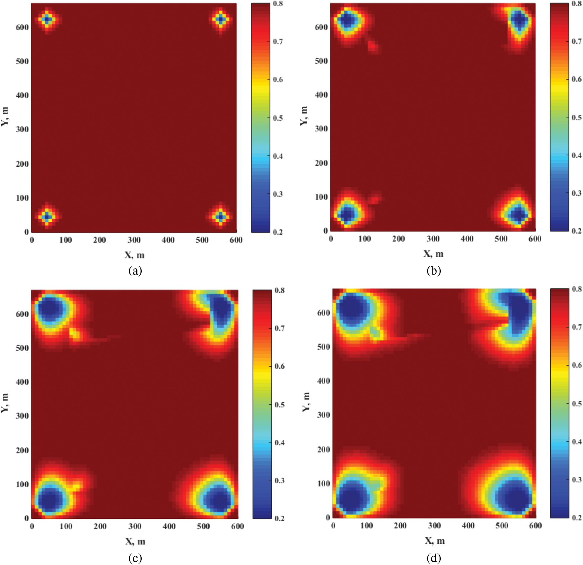
Figure 25: Oil saturation profiles of the upper layer (a) 50 days (b) 200 days (c) 500 days (d) 800 days

Figure 26: Oil saturation profiles of the lower layer (a) 50 days (b) 200 days (c) 500 days (d) 800 days

Figure 27: Production rates of the production well in this example (a) oil production rate (b) water production rate

7  Conclusions and Future Work

Throughout the whole paper, several key conclusions can be obtained:

(i) The original pEDFM fails to handle flow barriers in most cases due to unphysical fracture projection configurations, and determining the physical projection configuration of fractures is the critical step in pEDFM.

(ii) When determining the physical projection configuration, the focus should be on the entire fracture, not on individual fracture cells. Then, the equivalence theorem is presented and proved to explain the geometric equivalent nature of physical fracture projection configurations. The equivalence theorem-based pEDFM can truly handle cases where fracture permeability is lower than matrix permeability, especially flow barriers.

(iii) pEDFM can efficiently handle reservoir models with complex geological conditions (complex boundary shapes or inclined interlayers) by embedding flow barriers to flexibly ‘cut’ the reservoir models.

In addition, it should be pointed out that, the current topological theory seems to be applicable only to disjoint fractures (i.e., individual fractures), and a more general theory for intersecting fractures needs to be studied, which is deserving of significant future work. If topological theory, such as that discussed in this study, is still applied, it will be difficult to ensure that fluxes agree with the actual physical process of multiple fracture intersections.

Funding Statement: This work was supported by the National Natural Science Foundation of China (No. 52104017), and National Key Research and Development Program of China (Grant No. 2019YFA0705501), and State Center for Research and Development of Oil Shale Exploitation, and Cooperative Innovation Center of Unconventional Oil and Gas (Ministry of Education & Hubei Province), Yangtze University (No. UOG2020-17).

Conflicts of Interest: The authors declare that they have no conflicts of interest to report regarding the present study.

References

 1.  He, Y., Cheng, S., Sun, Z., Chai, Z., Rui, Z. (2020). Improving oil recovery through fracture injection and production of multiple fractured horizontal wells. Journal of Energy Resources Technology, 142(5), 053002. DOI 10.1115/1.4045957. [Google Scholar] [CrossRef]

 2.  Taleghani, A. D., Ahmadi, M. (2020). Thermoporoelastic analysis of artificially fractured geothermal reservoirs: A multiphysics problem. Journal of Energy Resources Technology, 142(8), 081302. DOI 10.1115/1.4045925. [Google Scholar] [CrossRef]

 3.  Xue, Y., Liu, J., Ranjith, P. G., Liang, X., Wang, S. (2021). Investigation of the influence of gas fracturing on fracturing characteristics of coal mass and gas extraction efficiency based on a multi-physical field model. Journal of Petroleum Science and Engineering, 206, 109018. DOI 10.1016/j.petrol.2021.109018. [Google Scholar] [CrossRef]

 4.  Xue, Y., Teng, T., Dang, F., Ma, Z., Wang, S. et al. (2020). Productivity analysis of fractured wells in reservoir of hydrogen and carbon based on dual-porosity medium model. International Journal of Hydrogen Energy, 45(39), 20240–20249. DOI 10.1016/j.ijhydene.2019.11.146. [Google Scholar] [CrossRef]

 5.  Slough, K. J., Sudicky, E. A., Forsyth, P. A. (1999). Grid refinement for modeling multiphase flow in discretely fractured porous media. Advances in Water Resources, 23(3), 261–269. DOI 10.1016/S0309-1708(99)00009-3. [Google Scholar] [CrossRef]

 6.  Karimi-Fard, M., Firoozabadi, A. (2001). Numerical simulation of water injection in 2D fractured media using discrete-fracture model. SPE Annual Technical Conference and Exhibition, OnePetro, New Orleans, Louisiana. [Google Scholar]

 7.  Karimi-Fard, M., Durlofsky, L. J., Aziz, K. (2004). An efficient discrete-fracture model applicable for general-purpose reservoir simulators. SPE Journal, 9(2), 227–236. DOI 10.2118/88812-PA. [Google Scholar] [CrossRef]

 8.  Fu, Y., Yang, Y. K., Deo, M. (2005). Three-dimensional, three-phase discrete-fracture reservoir simulator based on control volume finite element (CVFE) formulation. SPE Reservoir Simulation Symposium, The Woodlands, Texas. DOI 10.2118/93292-MS. [Google Scholar] [CrossRef]

 9.  Monteagudo, J. E. P., Firoozabadi, A. (2004). Control-volume method for numerical simulation of two-phase immiscible flow in two-and three-dimensional discrete-fractured media. Water Resources Research, 40(7), 7045. DOI 10.1029/2003WR002996. [Google Scholar] [CrossRef]

10. Alboin, C., Jaffré, J., Roberts, J. E., Serres, C. (2002). Modeling fractures as interfaces for flow and transport. Fluid Flow and Transport in Porous Media, Mathematical and Numerical Treatment, 295, 13. DOI 10.1090/conm/295/04999. [Google Scholar] [CrossRef]

11. Bahrainian, S. S., Dezfuli, A. D., Noghrehabadi, A. (2015). Unstructured grid generation in porous domains for flow simulations with discrete-fracture network model. Transport in Porous Media, 109(3), 693–709. DOI 10.1007/s11242-015-0544-3. [Google Scholar] [CrossRef]

12. Li, L., Lee, S. H. (2008). Efficient field-scale simulation of black oil in a naturally fractured reservoir through discrete fracture networks and homogenized media. SPE Reservoir Evaluation & Engineering, 11(4), 750–758. DOI 10.2118/103901-PA. [Google Scholar] [CrossRef]

13. Panfili, P., Cominelli, A. (2014). Simulation of miscible gas injection in a fractured carbonate reservoir using an embedded discrete fracture model. Abu Dhabi International Petroleum Exhibition and Conference, Abu Dhabi, UAE. DOI 10.2118/171830-MS. [Google Scholar] [CrossRef]

14. Shakiba, M., de Araujo Cavalcante Filho, J. S., Sepehrnoori, K. (2018). Using embedded discrete fracture model (EDFM) in numerical simulation of complex hydraulic fracture networks calibrated by microseismic monitoring data. Journal of Natural Gas Science and Engineering, 55, 495–507. DOI 10.1016/j.jngse.2018.04.019. [Google Scholar] [CrossRef]

15. Dachanuwattana, S., Jin, J., Zuloaga-Molero, P., Li, X., Xu, Y. et al. (2018). Application of proxy-based MCMC and EDFM to history match a Vaca Muerta shale oil well. Fuel, 220, 490–502. DOI 10.1016/j.fuel.2018.02.018. [Google Scholar] [CrossRef]

16. Norbeck, J. H., McClure, M. W., Lo, J. W., Horne, R. N. (2016). An embedded fracture modeling framework for simulation of hydraulic fracturing and shear stimulation. Computational Geosciences, 20(1), 1–18. DOI 10.1007/s10596-015-9543-2. [Google Scholar] [CrossRef]

17. Jiang, J., Younis, R. M. (2016). Hybrid coupled discrete-fracture/matrix and multicontinuum models for unconventional-reservoir simulation. SPE Journal, 21(3), 1009–1027. DOI 10.2118/178430-PA. [Google Scholar] [CrossRef]

18. Fumagalli, A., Scotti, A. (2013). A numerical method for two-phase flow in fractured porous media with non-matching grids. Advances in Water Resources, 62, 454–464. DOI 10.1016/j.advwatres.2013.04.001. [Google Scholar] [CrossRef]

19. Fumagalli, A., Zonca, S., Formaggia, L. (2017). Advances in computation of local problems for a flow-based upscaling in fractured reservoirs. Mathematics and Computers in Simulation, 137, 299–324. DOI 10.1016/j.matcom.2017.01.007. [Google Scholar] [CrossRef]

20. Cao, R., Fang, S., Jia, P., Cheng, L., Rao, X. (2019). An efficient embedded discrete-fracture model for 2D anisotropic reservoir simulation. Journal of Petroleum Science and Engineering, 174, 115–130. DOI 10.1016/j.petrol.2018.11.004. [Google Scholar] [CrossRef]

21. Xu, S. Q., Li, Y. Y., Zhao, Y., Wang, S., Feng, Q. H. (2020). A history matching framework to characterize fracture network and reservoir properties in tight Oil. Journal of Energy Resources Technology, 142(4), 042902. DOI 10.1115/1.4044767. [Google Scholar] [CrossRef]

22. Hajibeygi, H., Karvounis, D., Jenny, P. (2011). A hierarchical fracture model for the iterative multiscale finite volume method. Journal of Computational Physics, 230(24), 8729–8743. DOI 10.1016/j.jcp.2011.08.021. [Google Scholar] [CrossRef]

23. Moinfar, A., Varavei, A., Sepehrnoori, K., Johns, R. T. (2014). Development of an efficient embedded discrete fracture model for 3D compositional reservoir simulation in fractured reservoirs. SPE Journal, 19(2), 289–303. DOI 10.2118/154246-PA. [Google Scholar] [CrossRef]

24. Yan, X., Huang, Z., Yao, J., Li, Y., Fan, D. (2016). An efficient embedded discrete fracture model based on mimetic finite difference method. Journal of Petroleum Science and Engineering, 145, 11–21. DOI 10.1016/j.petrol.2016.03.013. [Google Scholar] [CrossRef]

25. Zhang, Q., Huang, Z., Yao, J., Wang, Y., Li, Y. (2017). Multiscale mimetic method for two-phase flow in fractured media using embedded discrete fracture model. Advances in Water Resources, 107, 180–190. DOI 10.1016/j.advwatres.2017.06.020. [Google Scholar] [CrossRef]

26. Zeng, Q., Liu, W., Yao, J. (2018). Hydro-mechanical modeling of hydraulic fracture propagation based on embedded discrete fracture model and extended finite element method. Journal of Petroleum Science and Engineering, 167, 64–77. DOI 10.1016/j.petrol.2018.03.086. [Google Scholar] [CrossRef]

27. Rao, X., Cheng, L., Cao, R., Jia, P., Dong, P. et al. (2019). A modified embedded discrete fracture model to improve the simulation accuracy during early-time production of multi-stage fractured horizontal well. SPE/IATMI Asia Pacific Oil & Gas Conference and Exhibition, Society of Petroleum Engineers, Bali, Indonesia. [Google Scholar]

28. Wu, Y., Cheng, L., Fang, S., Huang, S., Jia, P. (2020). A green element method-based discrete fracture model for simulation of the transient flow in heterogeneous fractured porous media. Advances in Water Resources, 136, 103489. DOI 10.1016/j.advwatres.2019.103489. [Google Scholar] [CrossRef]

29. Rao, X., Cheng, L., Cao, R., Jia, P., Wu, Y. et al. (2019). A modified embedded discrete fracture model to study the water blockage effect on water huff-n-puff process of tight oil reservoirs. Journal of Petroleum Science and Engineering, 181, 106232. DOI 10.1016/j.petrol.2019.106232. [Google Scholar] [CrossRef]

30. Li, L., Guo, X., Zhou, M., Chen, Z., Zhao, L. et al. (2021). Numerical modeling of fluid flow in tight oil reservoirs considering complex fracturing networks and Pre-Darcy flow. Journal of Petroleum Science and Engineering, 207, 109050. DOI 10.1016/j.petrol.2021.109050. [Google Scholar] [CrossRef]

31. Ţene, M., Bosma, S. B., Al Kobaisi, M. S., Hajibeygi, H. (2017). Projection-based embedded discrete fracture model (pEDFM). Advances in Water Resources, 105, 205–216. DOI 10.1016/j.advwatres.2017.05.009. [Google Scholar] [CrossRef]

32. Jiang, J., Younis, R. M. (2017). An improved projection-based embedded discrete fracture model (pEDFM) for multiphase flow in fractured reservoirs. Advances in Water Resources, 109, 267–289. DOI 10.1016/j.advwatres.2017.09.017. [Google Scholar] [CrossRef]

33. Rao, X., Cheng, L., Cao, R., Jia, P., Liu, H. et al. (2020). A modified projection-based embedded discrete fracture model (pEDFM) for practical and accurate numerical simulation of fractured reservoir. Journal of Petroleum Science and Engineering, 187, 106852. DOI 10.1016/j.petrol.2019.106852. [Google Scholar] [CrossRef]

34. Liu, H., Rao, X., Xiong, H. (2020). Evaluation of CO2 sequestration capacity in complex-boundary-shape shale gas reservoirs using projection-based embedded discrete fracture model (pEDFM). Fuel, 277, 118201. DOI 10.1016/j.fuel.2020.118201. [Google Scholar] [CrossRef]

35. Olorode, O., Wang, B., Rashid, H. U. (2020). Three-dimensional projection-based embedded discrete-fracture model for compositional simulation of fractured reservoirs. SPE Journal, 25(4), 2143–2161. DOI 10.2118/201243-PA. [Google Scholar] [CrossRef]

36. Ren, G., Jiang, J., Younis, R. M. (2018). A model for coupled geomechanics and multiphase flow in fractured porous media using embedded meshes. Advances in Water Resources, 122, 113–130. DOI 10.1016/j.advwatres.2018.09.017. [Google Scholar] [CrossRef]

37. Ren, G., Younis, R. M. (2021). An integrated numerical model for coupled poro-hydro-mechanics and fracture propagation using embedded meshes. Computer Methods in Applied Mechanics and Engineering, 376, 113606. DOI 10.1016/j.cma.2020.113606. [Google Scholar] [CrossRef]

38. Rao, X., Xin, L., He, Y., Fang, X., Gong, R. et al. (2022). Numerical simulation of two-phase heat and mass transfer in fractured reservoirs based on projection-based embedded discrete fracture model (pEDFM). Journal of Petroleum Science and Engineering, 208, 109323. DOI 10.1016/j.petrol.2021.109323. [Google Scholar] [CrossRef]

39. Armstrong, M. A. (2013). Basic topology, Springer Science & Business Media. [Google Scholar]

40. Rao, X., Xu, Y., Liu, D., Liu, Y., Hu, Y. (2022). A general physics-based data-driven framework for numericalsimulation and history matching of reservoirs. Advances in Geo-Energy Research, 5(4), 422–436. DOI 10.46690/ager.2021.04.07. [Google Scholar] [CrossRef]

This work is licensed under a Creative Commons Attribution 4.0 International License, which permits unrestricted use, distribution, and reproduction in any medium, provided the original work is properly cited.