Computer Modeling in Engineering & Sciences

DOI: 10.32604/cmes.2022.018540

ARTICLE

Nonlinear Response of Tunnel Portal under Earthquake Waves with Different Vibration Directions

Hongyun Jiao1, Mi Zhao1, Jingqi Huang2,*, Xu Zhao1,3 and Xiuli Du1

1Key Laboratory of Urban Security and Disaster Engineering of Ministry of Education, Beijing University of Technology, Beijing, 100124, China
2Beijing Key Laboratory of Urban Underground Space Engineering, School of Civil and Resource Engineering, University of Science and Technology Beijing, Beijing, 100083, China
3Beijing Key Laboratory of Earthquake Engineering and Structural Retrofit, Beijing University of Technology, Beijing, 100124, China
*Corresponding Author: Jingqi Huang. Email: huangjingqi11@163.com
Received: 01 August 2021; Accepted: 22 November 2021

1  Introduction

The thousands of mountain tunnels that have recently been built in China play an important role in local development. Such tunnels may pass through highly active seismic areas, especially in Southwest China. Several strong earthquakes in recent decades, some mountain tunnel portals suffered particularly serious damage to some mountain tunnel portals, which is just less critical than that of the fault [1–4]. Slope instability, rock collapse and lining cracks are triggered by strong earthquakes, introducing numerous challenges to the safe operation of these tunnels. Thus, the tunnel portal is one of the weaker components of the tunnel structure in the event of an earthquake [5,6].

There has been considerable research on the seismic damage suffered by tunnel portals, mainly through model tests, numerical simulations, and in-situ investigations. Sun et al. [7] performed model tests to investigate the seismic response of a tunnel portal, and analyzed the interface interaction characteristics of the surrounding rock and the tunnel lining. To study the failure mode of a tunnel portal under strong earthquakes, Zhao et al. [8] adopted a rigid box model performed shaking table tests of the tunnel portal section. Xu et al. [9] conducted further shaking table tests to study the seismic response of the tunnel portal under different seismic scenarios. Compared with model tests, numerical simulations require less time and labor resources, and are capable of simulating a larger range of environmental and boundary conditions. Wu et al. [10] studied the damage mechanisms of a tunnel portal numerically, while Liu et al. [11] conducted a numerical study of the seismic response of the tunnel portal at the Dianzhong water diversion project. Importantly, Wang et al. [12] proved that the hydrodynamic pressure has a significant adverse effect on the seismic capacity of the tunnel portal. Other excellent research has been reported by Geni [13] and Yu et al. [14], Yu et al. [15] and so on. These preliminary works make us have more knowledge of the seismic performance and failure mechanism of the tunnel portals.

Because of the smaller overburden depth, the tunnel portal has a seismic response that is strongly affected by the slope around the structure. The slope rock is often severely weathered, reducing its ability to restrain the portal structure compared with other tunnel parts that are buried deeper underground [12]. Therefore, a precise and appropriate constitutive model is essential in simulating the failure strength, plastic deformation, damage softening, and other seismic mechanical behavior of slope rock. However, previous works have only considered heavily simplified constitutive models, such as linear elastic models, plastic models based on the Mohr–Coulomb criterion, and so on. Moreover, earthquake waves propagate through the ground in different vibration directions. Although many researchers have studied the seismic response of deep-buried tunnels under earthquake waves propagating in different vibration direction [16–19], the seismic response and damage characteristics of tunnel portals under such conditions have not been fully considered.

In this study, an elastoplastic damage model is integrated into the ABAQUS software through a self-compiled user material (UMAT) subroutine, allowing the mechanical behavior of the slope rock to be simulated. First, the accuracy of the model is verified. Based on the Galongla tunnel project, a dynamic time-history model is then constructed to simulate the seismic response. A viscous-spring boundary is used to absorb the wave radiation. In addition, a wave input method for the slope rock is established, and the applicability and accuracy of this method are verified. Vertical incident seismic waves in different vibration directions are simulated by the proposed method, and the response of the portal structure of Galongla tunnel is numerically studied. Finally, the seismic response characteristics and damage mechanism of the tunnel portal are discussed.

2  Galongla Tunnel Project

Galongla tunnel is a critical part of the Zhamo highway in Tibet, the only highway leading to Motuo County in China. the local geography is shown in Fig. 1a. The geological condition of the tunnel is very complex. As shown in the geological profile in Fig. 1b, the rock mass along the tunnel can be divided into Grades II, III, and IV according to the Chinese rock classification code. The tunnel portal is loose Holocene deposits consisting of welded tuff, gravel, silt, and clay, as shown in Fig. 1c. The cross-section of the Galongla tunnel is horseshoe shaped, as shown in Fig. 2. The tunnel structure consists of rock bolts, a primary lining, a waterproof layer, and a secondary lining, and was excavated and constructed by the New Austrian tunneling method.

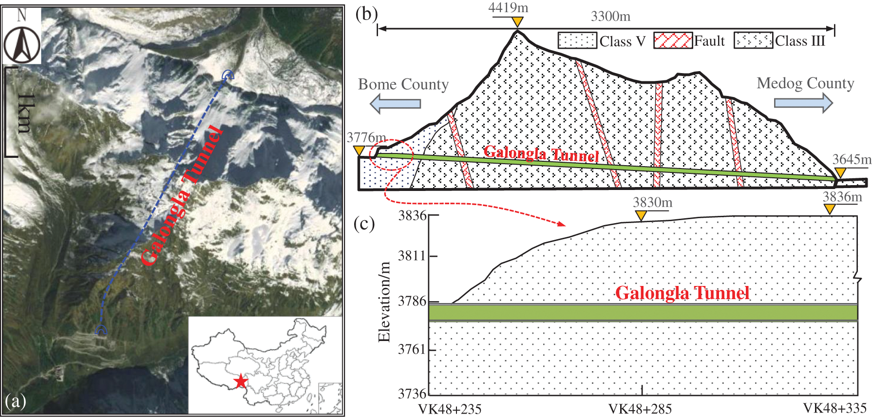
Figure 1: Sketch of Galongla tunnel: (a) satellite image around Galongla tunnel; (b) longitudinal profile; and (c) portal section

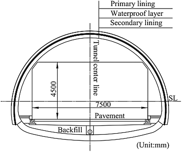
Figure 2: Cross-section of Galongla tunnel portal

Galongla tunnel is located in the Himalayan fault zone, which is subjected to frequent geological activity, i.e., an earthquake-prone area. According to the seismic data issued by the China Earthquake Administration, the basic intensity degree is VIII. Therefore, the tunnel, especially the tunnel portal, faces a serious earthquake risk. To investigate the seismic damage mechanics of the tunnel portal part, the results of dynamic numerical analysis are described in the following sections.

3  Elastoplastic Damage Model for Rocks and Realization with the ABAQUS Software

Based on the nonlinear unified strength criterion, Du et al. [20] established a triaxial elastoplastic damage model for rock mass. The plastic part of the model employs the nonlinear unified strength criterion as the yield function in the effective stress space. The hardening law takes the equivalent plastic shear strain as the hardening parameter, and considers the effect of mean stress on the hardening rate. For the damage part, the evolution law is assumed to have an exponential form so as to consider the degradation and softening behavior of the rock mass. In this study, the constitutive model is implemented in the ABAQUS software through a self-compiled UMAT subroutine to simulate the mechanical behavior of the rock mass [21].

3.1 Description of the Elastoplastic Damage Model

The following nonlinear unified strength criterion developed by Lu et al. [22] is adopted as the yield function of the plastic part:

f(σ¯ij,κ)=22(σ^1−σ^2)2+(σ^2−σ^3)2+(σ^3−σ^1)2−κMβσ^1+σ^2+σ^33(1)

where κ is the hardening variable; σ^i and Mβ are the characteristic stress and the failure strength ratio, respectively, which can be expressed as

{σ^i=pr(σ¯ipr)βMβ=3(1+sin⁡ϕc)β−(1−sin⁡ϕc)β(1+sin⁡ϕc)β+2(1−sin⁡ϕc)β(2)

where the reference stress pr takes a value of 1 MPa to give a dimensionless stress; β denotes the parameter for converting the normal stress σ¯i to the characteristic stress σ^i, which is constant for a certain material; φc denotes the internal friction angle.

To describe the rock dilatancy effectively, a non-associated flow rule is adopted. The expression for the plastic potential function is similar to the yield function, with the parameter Mβ replaced by Mg, which is a function of the dilatancy angle ψ:

Mg=3(1+sin⁡ψ)β−(1−sin⁡ψ)β(1+sin⁡ψc)β+2(1−sin⁡ψ)β(3)

The hardening variable κ is a function of the equivalent plastic shear strain γp, and has the form

κ={∫dκ if κ<11 if κ≥1,dκ=3(1−ao)(1−κ1−ao)23Aγp+σ0σc/3+σ0dγp(4)

where ao is the initial hardening rate; σcand σo are the uniaxial compression strength and the three-dimensional tensile strength, respectively; and Aγ is the plastic shear strain corresponding to the hydrostatic pressure p, which has a value of σc/3. The equivalent plastic shear strain γp can be calculated as

γp=23deijpdeijp=23(εijp−13εvpδij)(εijp−13εvpδij)(5)

where eijp is the plastic deviatoric strain; εijp and εvp denote the plastic strain tensor and the plastic volume strain, respectively; δij is Kronecker's delta.

The damage factor d is introduced to characterize the micro-defects in the surrounding rock material and the development of its internal damage state. There are two main forms of the damage factor, i.e., scalar damage variables and tensor damage variables. The damage variable in scalar form describes the isotropic damage of a material, and is mainly used for the distribution of spherical defects. It is considered that the damage degree of a material is the same in any direction. However, the direction of crack propagation for rock materials often has a certain directionality under the action of external load, and the influence of these cracks on the cross-sectional area will be different in each direction. Given the anisotropy of rock damage, many researchers use tensor damage variables to characterize the directionality of crack distribution and propagation. In establishing a rock damage evolution equation, many scholars have established models based on different damage internal variables [23–33]. Considering that the rock damage is softened by the volume expansion caused by the development of internal micro-cracks, this paper uses the volume strain as the internal variable of the evolution of damage. The specified damage variable is positive in compression and negative in tension. In the damage part of the model, the damage variable d is defined as

d=1−exp⁡(−b1εd)(6)

where b1 is a parameter controlling the slope of the softening curve; εd is the equivalent strain, which can be written as

εd=∫ε˙dε˙d={ 0if κ<1ε˙pv(σ33+|σ33|pr+1)b2ifκ≥1ε˙pv=∑i=13〈−ε˙pi〉(7)

where dεpv is the volumetric plastic strain rate; χ1 controls the rate of increase of εd; b2 is a constant that affects the value of χ1.

3.2 Relationship between the Stress and Strain

For the elastoplastic damage model, the increment in the Cauchy stress σij can be expressed as the effective stress σ¯ij:

dσij=(1−d)dσ¯ij(8)

The relationship between increments in the effective stress σ¯ij and the stain εij is

dσ¯ij=Dijkledεije=Dijkle(dεij−dεijp)(9)

where εije and εijp denote the elastic strain and the plastic strain, respectively; Dijkle is the elastic stiffness matrix, which has the form

Dijkle=E2(1+v)(δikδjl+δilδjk)+vE(1+v)(1−2v)δijδkl(10)

The plastic strain increment dεijp can be obtained by the following flow rule:

dεijp=dλ∂g∂σij(11)

Substituting Eq. (11) into Eq. (5) yields

dγp=23(∂g∂σij−13∂g∂σkkδij)(∂g∂σij−13∂g∂σkkδij)dλ(12)

The consistency condition then gives

df=∂f∂σijdσ¯ij+∂f∂γpdγp=0(13)

Substituting Eq. (12) into Eq. (13), we obtain

dλ=∂f∂σ¯ijdσ¯ijA(14)

where

A=−∂f∂γp23(∂g∂σ¯ij−13∂g∂σ¯kkδij)(∂g∂σ¯ij−13∂g∂σ¯kkδij)(15)

Combining Eqs. (9), (11), and (14), we find that

dλ=∂f∂σ¯ijDijkleA+∂f∂σ¯ijDijkle∂g∂σ¯kldεij(16)

Combining Eqs. (9), (11), and (16) gives, after some rearrangement, the stress–strain increment relationship:

dσij=(1−d)(Dijkle−Dijkle∂g∂σ¯ij∂f∂σ¯klDijkleA+∂f∂σ¯ijDijkle∂g∂σ¯kl)dεij(17)

The expressions for ∂f∂γp, ∂f∂σ¯ij, and ∂g∂σ¯ij in Eqs. (15) and (17) are given in the Appendix.

3.3 Implementation in ABAQUS Software and Verification

Based on the derived relationship between the stress and strain, the elastoplastic damage model is integrated into the ABAQUS software through a self-developed UMAT subroutine. To verify the accuracy of the implemented model, a three-dimensional (3-D) solid unit cube model measuring 1 m × 1 m × 1 m is built and discretized into a single grid using reduction integral elements (C3D8R). The numerical results are compared with the results of conventional triaxial experiments by Kawamoto et al. [34] and Lin et al. [35]. The constitutive model parameters of the triaxial experiments performed by Kawamoto et al. [34] and Lin et al. [35] are listed in Table 1.

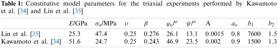
Fig. 3 compares the results obtained by the present model and those reported by Kawamoto et al. [34] and Lin et al. [35]. From this figure, it is clear that the constitutive model accurately simulates the whole process of rock deformation and damage under a complex stress state, especially the strain softening and the changing characteristics of strength with respect to the confining pressure.

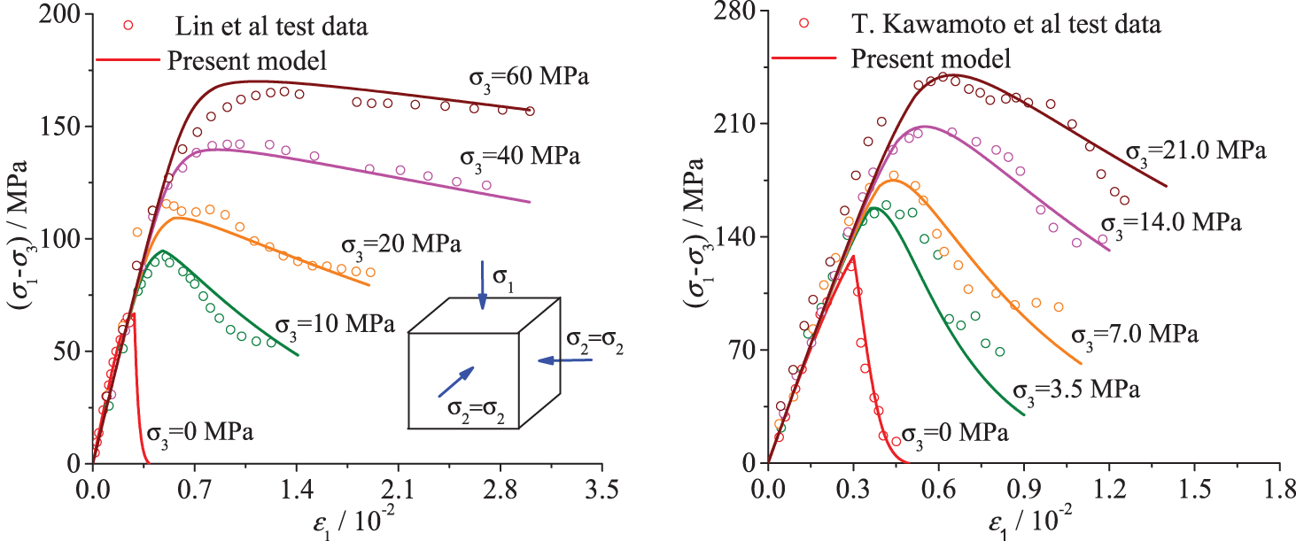
Figure 3: Comparison between the present model and the triaxial experiments performed by Kawamoto et al. [34] and Lin et al. [35]

4  Dynamic Finite Element Model

4.1 Geometry of the Computational Model

To investigate the seismic response of the Galongla tunnel portal, dynamic history simulations were performed using the ABAQUS software. The 3-D finite element model and its dimensions are shown in Fig. 4, in which the slope inclination is set to be 4:5 in height and length along the tunnel axial direction. The Mohr–Coulomb constitutive model was adopted for the nonlinear behavior of the tunnel lining, with material parameters of density ρ = 2500 kg/m3, Young's modulus E = 30 GPa, Poisson's ratio υ = 0.22, friction angle φ = 58.7°, and cohesive stress c = 2.3 MPa. The rock medium was simulated by the elastoplastic damage model, implemented in the ABAQUS software as described in Section 3, with material parameters of ρ = 2300 kg/m3, E = 0.87 GPa, υ = 0.42, β = 0.225, σo = 24.7 MPa, φc = 46.9, ψ = 23.5, A = 0.0018, ao = 0.9, b1 = 501, b2 =1.07.

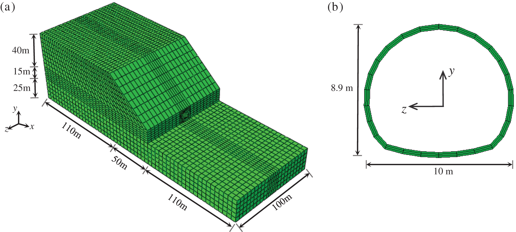
Figure 4: 3-D computational model of Galongla tunnel portal: (a) rock mass; (b) tunnel structure

In this study, the tunnel portal responses under three different earthquake incident waves are investigated. The first case considers the incident waves to be plane P waves with a vibration direction perpendicular to the tunnel axis. The second and third cases consider the earthquake waves to be vertically incident S waves with vibration directions perpendicular and parallel to the tunnel axis, respectively. The Kobe University earthquake records for rock strata were obtained in similar geological conditions to those of the Galongla tunnel project site. The Kobe waves are real seismic records with rich spectra, as shown in Fig. 5. They have been widely used to study the seismic response of mountain tunnels through numerical simulations and experimental tests. Therefore, the Kobe waves are selected as the input waves in this study.

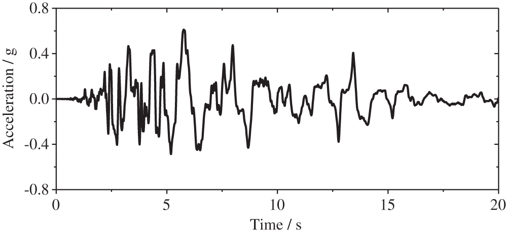
Figure 5: Acceleration time histories of the incident earthquake waves

During the numerical analysis, a viscous-spring artificial boundary is employed to simulate the radiation damping effect at the truncated boundary, as introduced in Section 4.2. The seismic input method for the slope site considering different vibration directions is then described in Section 4.3.

4.2 Viscous-Spring Artificial Boundary

In recent decades, many artificial boundaries have been developed which can be found in the works of Lysmer et al. [36], Deeks et al. [37], Du et al. [38], and so on. The viscous-spring boundary developed by Du et al. [38] is adopted in this study due to its simple form and high accuracy. The boundary is realized by establishing springs and dampers in three directions, as shown in Fig. 6a. At boundary node l of the 3-D finite element model, the parameters of the springs and dashpots are

{K3ln=1(1+ar)λ+2GR,C3ln=brρcpK3ls=1(1+ar)GR,C3ls=brρcs(18)

where the subscripts n and s denote the normal and tangential direction of the boundary plane, respectively. The distance between the wave source and the artificial boundary is denoted by R; λ, G, and ρ denote the Lamé constant, shear modulus, and mass density, respectively; cs is the shear wave velocity in the medium, and cp is the compression wave velocity; ar and br denote the modified coefficients, which have values of 0.8 and 1.1, respectively.

4.3 Seismic Input Method

Fig. 6a describes the incident conditions for the truncated region of the slope site. The earthquake wave motions can be converted into equivalent nodal forces, which are applied at the artificial boundary [39–41]. Together with the viscous-spring boundary developed by Du et al. [38], the equivalent nodal forces at a given boundary node l can be obtained from Eqs. (19)–(21). The specific forms are as follows.

For node l on the bottom boundary (y = 0), the equivalent nodal forces are

{Fx=A3l(K3lsux+C3lsu˙x−σyx)Fy=A3l(K3lnuy+C3lnu˙y−σyy) Fz=A3l(K3lsuz+C3lsu˙z−σyz)(19)

where Fx, Fy, and Fz are the equivalent nodal forces in the x, y, and z directions, respectively; ux, uy, and uz are the free field displacements of boundary node l in the x, y, and z directions, respectively; u˙x, u˙y, and u˙z are the free field velocities; σyy, σyx, and σyz are the free field stresses; A3l is a quarter of the total area of all boundary elements containing boundary node l, as shown in Fig. 6a, where A3l = (A1 + A2 + A3 + A4)/4.

For node l on the left boundary (x = 0) and the right boundary (x = Lx), the equivalent nodal forces are

{Fx=A3l(K3lnux+C3lnu˙x+δσxx)Fy=A3l(K3lsuy+C3lsu˙y+δσxy) Fz=A3l(K3lsuz+C3lsu˙z+δσzx)(20)

where δ is a boundary-dependent parameter, i.e., δ = −1 for the left boundary and δ = 1 for the right boundary; σxx, σxy, and σxz are the free field stresses on the left and right boundaries, respectively.

For node l on the back boundary (z = 0) and the front boundary (z = Lz), the equivalent nodal forces are

{Fx=A3l(K3lsux+C3lsu˙x+δσzx)Fy=A3l(K3lsuy+C3lsu˙y+δσzy) Fz=A3l(K3lnuz+C3lnu˙z+δσzz)(21)

where δ takes a value of −1 on the back boundary and a value of 1 on the front boundary; σzz, σzx, and σzy are the free field stresses on the front and back boundaries, respectively.

As shown in Eqs. (19)–(21), the free field displacements ux, uy, and uz, velocities ..., u˙y, and u˙z, and stresses σxx, σyy, σzz, σxy, σzy, and σzx need to be determined to calculate the boundary equivalent nodal forces. The free field displacements, velocities, and stresses of each boundary node can be determined through free field site analysis. In consideration of the homogeneity and isotropy of the site and the symmetry of the loading conditions, the free field response of the slope site can be analyzed using a two-dimensional (2-D) site model, as shown in Fig. 6b.

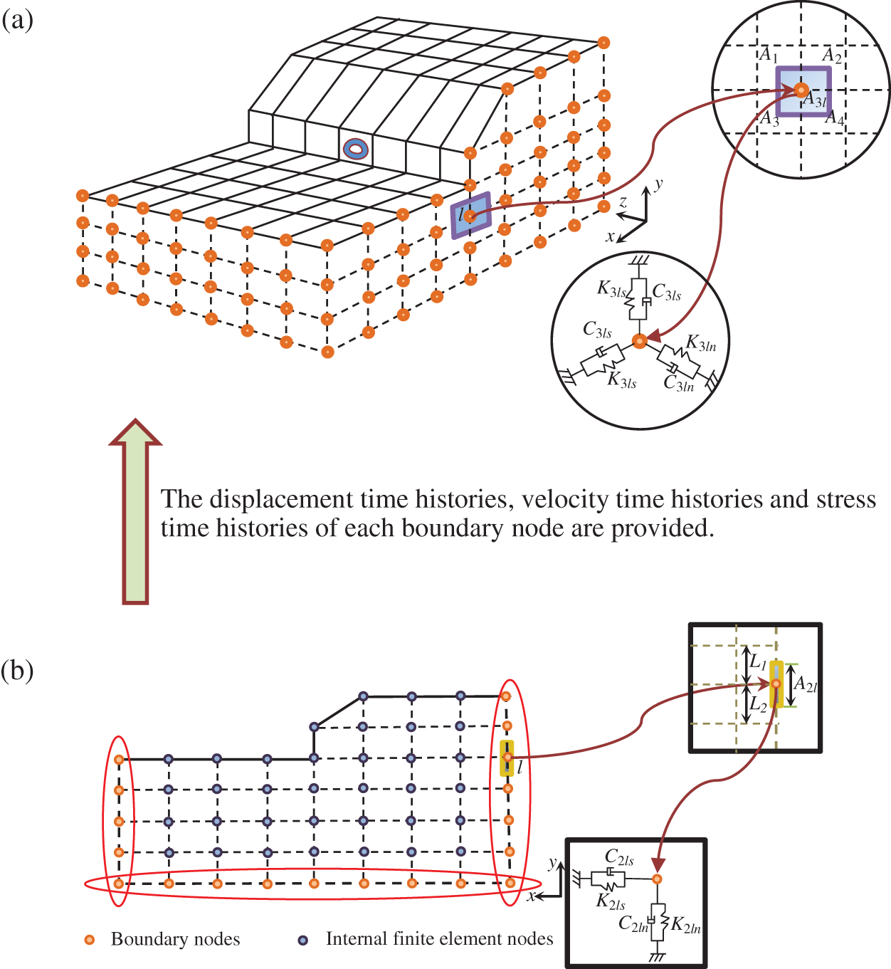
Figure 6: Illustration of the seismic input method for the 3-D slope site

In the 2-D model for slope seismic analysis, the viscous-spring boundary developed by Du et al. [38] is applied at the bottom and lateral boundaries. At boundary node l of the 2-D model, the spring and dashpot parameters can be written as

{K2ln=1(1+ar)λ+2G2R,C2ln=brρcpK2ls=1(1+ar)G2R,C2ls=brρcs(22)

In addition, the incident earthquake waves are converted into equivalent nodal forces that apply at each boundary node. For node l on the bottom boundary (y = 0) of the 2-D model, the equivalent nodal forces of incident SV, SH, and P waves are given by

{ Fx=A2l(K2lsu0(t)+Gcsu˙0(t))Fy=Fz=0SVwave(23a)

{ Fx=Fy=0Fz=A2l(K2lsu0(t)+Gcsu˙0(t))SHwave (23b)

{ Fx=Fz=0Fy=A2l(K2lnu0(t)+λ+2Gcpu˙0(t))Pwave (23c)

where u0(t) and u˙0(t) denote the displacement and velocity of the incident waves. A2l is half of the total length of all boundary elements containing boundary node l in the 2-D finite element model, as shown in Fig. 6b, where A2l = (L1 + L2)/2.

For node l on the left boundary (x = 0) and the right boundary (x = Lx), the equivalent nodal forces of the incident waves are given by

{ Fx=A2l[ K2ln(u0(t)+u0(t−2h−ylcs))+C2ln(u˙0(t)+u˙0(t−2h−ylcs)) ]Fy=A2lGcsδ(u˙0(t)−u˙0(t−2h−ylcs))Fz=0SVwave (24a)

{ Fx=Fy=0Fz=A2l[ K2ls(u0(t)+u0(t−2h−ylcs))+C2ls(u˙0(t)+u˙0(t−2h−ylcs)) ]SHwave(24b)

{ Fx=A2lλcpδ(u˙0(t)−u˙0(t−2h−ylcp))Fy=A2l[ K2ls(u0(t)+u0(t−2h−ylcp))+C2ls(u˙0(t)+u˙0(t−2h−ylcp)) ]Fz=0Pwave (24c)

where the boundary-dependent parameter δ takes a value of −1 on the left boundary and a value of 1 on the right boundary; h is the height of the lateral boundary.

In general, the seismic input method for the 3-D model is as illustrated in Fig. 6. First, the free field response of the slope site is numerically simulated by a 2-D site model. Using the displacement, velocity, and stress time histories from the 2-D site model, the equivalent nodal forces of the 3-D model are calculated with Eqs. (19)–(21).

4.4 Validation of Seismic Input Method

The proposed seismic input method is now verified. The 3-D slope site model illustrated in Fig. 7 was constructed with material parameters of ρ = 2300 kg/m3, E = 0.87 GPa, and υ = 0.42. The input seismic waves take the form of an impulse, with the displacement time history shown in Fig. 8. With the aid of the present seismic input method, the impulse is transmitted to the 3-D slope site model as vertically incident P waves and vertically incident S waves with vibration directions perpendicular and parallel to the x-direction, respectively. In addition, a 2-D slope site model was constructed to provide reference solutions.

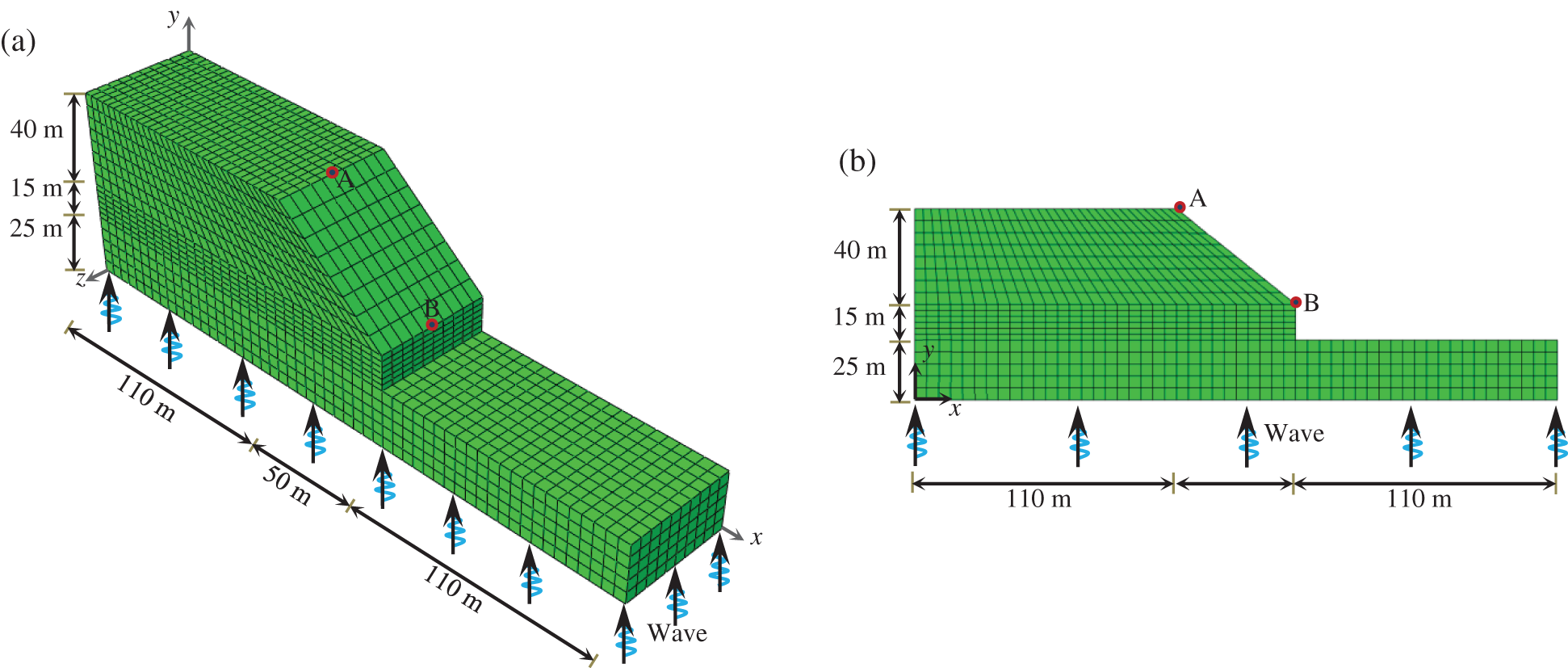
Figure 7: Calculation model (a) the 3-D model (b) the 2-D model

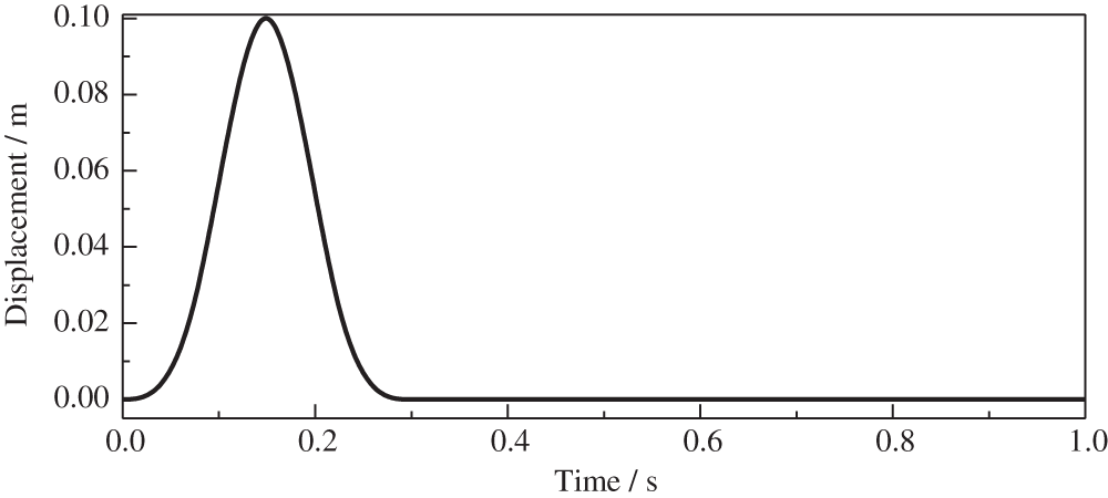
Figure 8: Displacement time history of input seismic waves

The displacement contours of the 2-D model and the 3-D model are compared in Fig. 9. For reasons of brevity, only the displacement contours under vertically incident P waves are shown in this figure. It can be observed from Fig. 9 that the displacement contours of the 3-D model are very similar to those of the 2-D model. Moreover, the displacement in the y-direction at monitoring points A and B is plotted in Fig. 10. From Fig. 10, it is apparent that the 3-D model provides good agreement with the 2-D model. Thus, the incident method of the 3-D slope site proposed in this paper has a high degree of accuracy, and can thus be employed to investigate the seismic response of the tunnel portal.

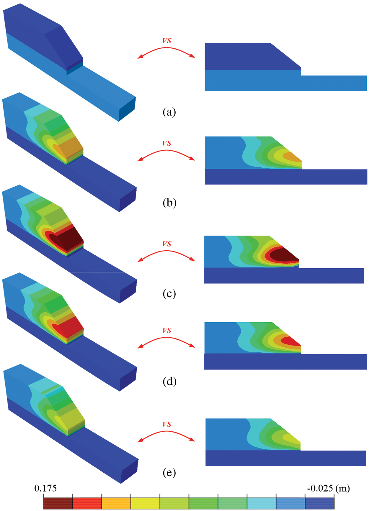
Figure 9: Comparison of displacement contours of the 2-D model and the 3-D model under P waves (a) t = 0.05 s (b) t = 0.15s (c) t = 0.25 s (d) t = 0.30 s (e) t = 0.40 s

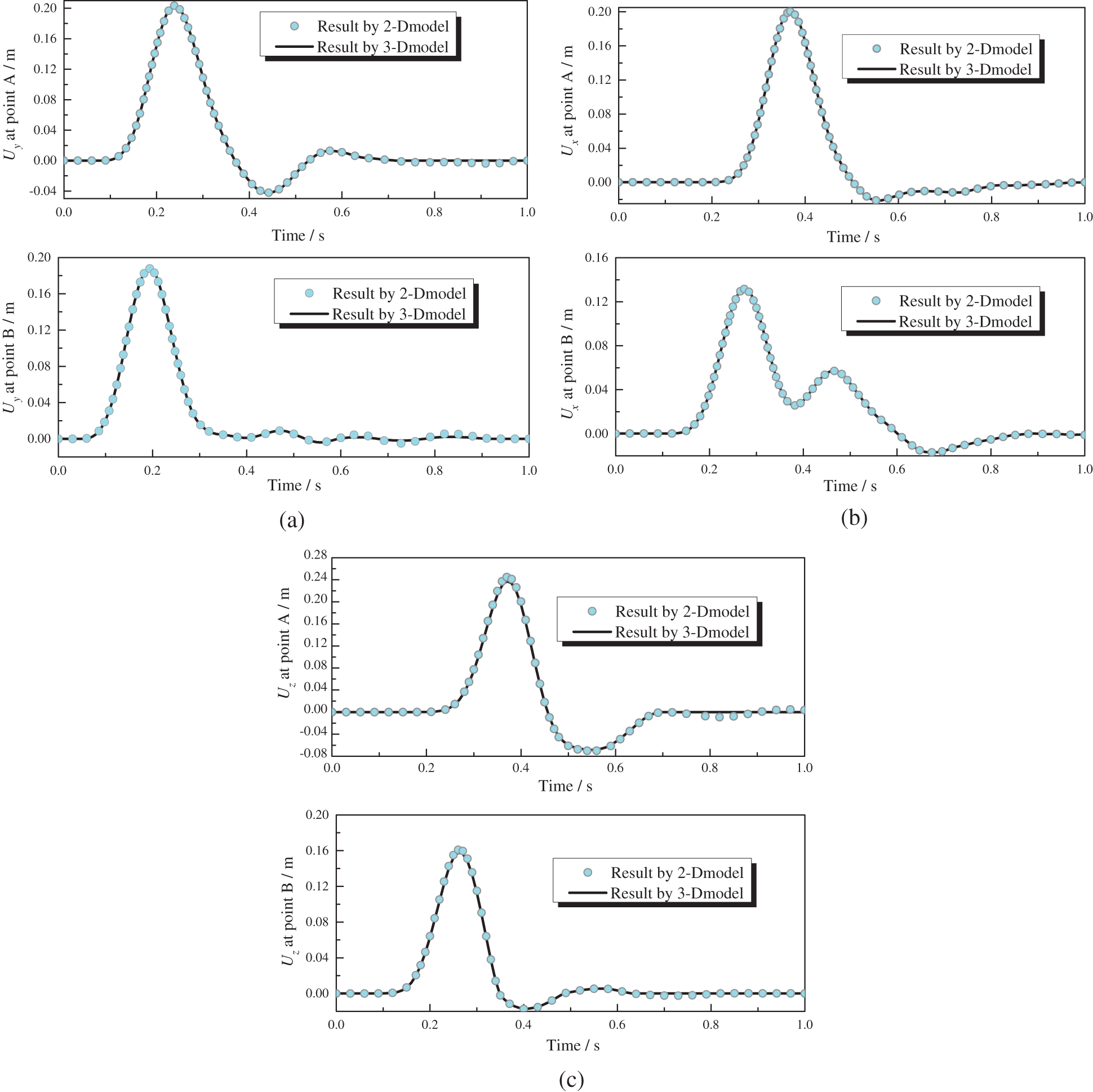
Figure 10: Displacement time histories at points A and B (a) P waves with vibration direction being perpendicular to the tunnel axis (b) S waves with vibration direction being parallel to the tunnel axis (c) S waves with vibration direction being perpendicular to the tunnel axis

5  Numerical Results

5.1 Vertically Incident S Waves with Vibration Direction Perpendicular to Tunnel Axis

Fig. 11 shows the damage factor contours of the rock ground near the tunnel portal under S waves with a vibration direction perpendicular to the tunnel axis. The surrounding rock suffers heavy damage, especially near the tunnel–ground interface. The damage to the surrounding rock near the tunnel foot and spandrel is significant near the tunnel entrance. With increasing distance from the entrance, the heavy damage gradually shifts from the tunnel foot and spandrel to the tunnel vault and bottom.

Figure 11: Damage factor contours of rock ground near the tunnel portal under S waves with vibration direction perpendicular to tunnel axis

The maximum principal plastic strain contours of the tunnel lining under S waves with a vibration direction perpendicular to the tunnel axis is presented in Fig. 12. The dynamic response of the tunnel lining is mainly affected by the tunnel–foundation interactions, the mechanics of which are significantly different from those of upper structures built on open land. Thus, the plastic deformation of the tunnel matches the progress of damage in the surrounding rock (see Fig. 11). In detail, at the tunnel entrance, the plastic strain is concentrated around the tunnel foot and spandrel. With increasing distance from the entrance, the plastic strain shifts from the tunnel foot and spandrel to the tunnel vault and bottom.

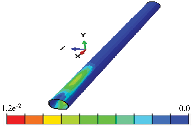
Figure 12: Maximum principal plastic strain of the tunnel lining under S waves with vibration direction perpendicular to tunnel axis

The strain can be decomposed into the hoop axial strain εh, hoop shear strain γh, and axial tensile strain εa, as shown in Fig. 13. Fig. 14 shows the distributions of these strain components at tunnel cross-sections of D = 7.5 m and 61.5 m, respectively, using L-foot to represent the lower left arch foot position of the lining, using L-haunch to represent the left arch waist position of the lining, using L-spandrel to represent the upper left arch shoulder position of the lining, using R-foot to represent the lower right arch foot position of the lining, using R-haunch to represent the right arch waist position of the lining, using R-spandrel to represent the upper right arch shoulder position of the lining, using Bottom to represent the bottom center position of the lining, and using Vault to represent the top center position of the lining. The same goes in the following. Significant hoop axial strain εh appears at the tunnel foot and spandrel, and the hoop shear strain γh around the tunnel bottom and vault is considerable. Though the rock-tunnel model is bilaterally symmetric, the shaking produced by an earthquake is not symmetric, and neither are the vertically incident S waves with a vibration direction perpendicular to the tunnel axis. Thus, εh and γh are not symmetric at the cross-sections. Compared with εh and εh, the axial tensile strain εa is very small, which indicates that the tunnel suffers only slight tensile deformation in the tunnel axial direction.

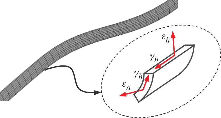
Figure 13: Illustration of the strain components

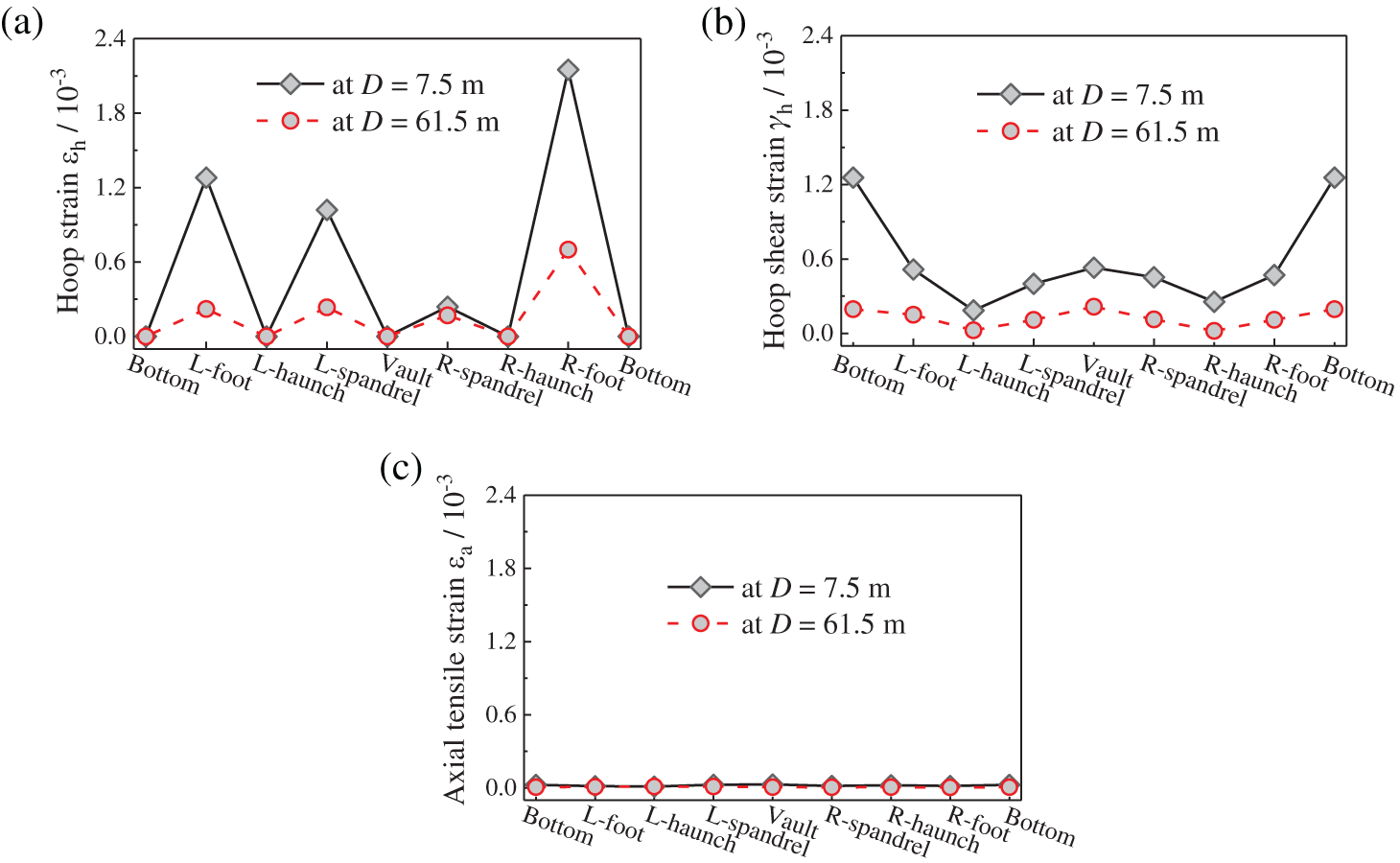
Figure 14: Distribution of strain components along lining cross section for S waves with vibration direction perpendicular to tunnel axis: (a) hoop strain, (b) hoop shear strain, and (c) axial tensile strain

The distributions of hoop axial strain εh at the left spandrel and right arch foot along the tunnel axis are given in Fig. 15a, and the hoop shear strain γh at the tunnel vault and bottom are shown in Fig. 15b. As the axial tensile strain εa is very small, the distribution of this component along the tunnel axis is not presented. From Fig. 15a, εh at the spandrel and arch foot are dominant at the tunnel entrance, and then quickly decrease to a stable value with distance from the tunnel entrance. Therefore, the plastic strain at the spandrel and arch foot are higher around the tunnel entrance than at other positions, as shown in Fig. 12. Fig. 15b shows that the hoop shear strain first increases and then decreases with increasing distance from the tunnel entrance. Thus, the plastic damage changes to become concentrated around the tunnel vault and bottom, as shown in Fig. 12.

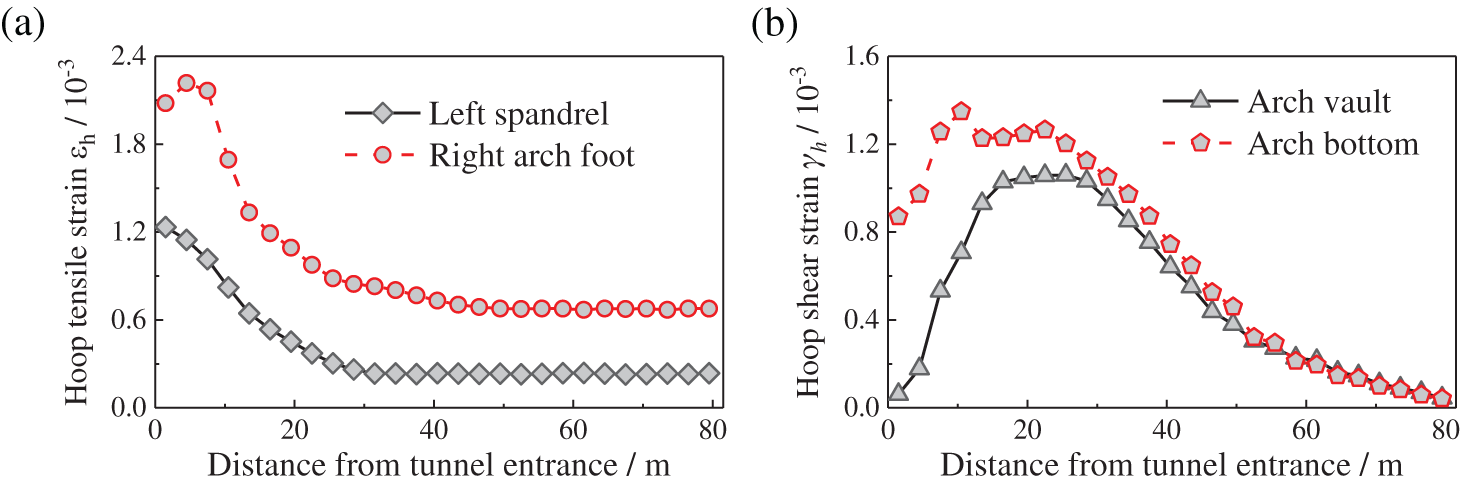
Figure 15: Distributions of strain components along the tunnel axis for S waves with vibration direction perpendicular to tunnel axis: (a) hoop axial strain and (b) hoop shear strain

5.2 Vertically Incident S Waves with Vibration Direction Parallel to Tunnel Axis

Fig. 16 shows the damage factor contours of the rock ground near the tunnel portal under S waves with a vibration direction parallel to the tunnel axis. The surrounding rock suffers severe damage near the tunnel entrance. Moreover, the damage contours of the rock are symmetrical. Fig. 17 shows the maximum principal plastic strain contour at the tunnel lining under S waves with a vibration direction parallel to the tunnel axis. The plastic strain of the tunnel lining in Fig. 17 is concentrated around the tunnel haunches, and the value increases and then decreases with distance from the tunnel entrance. Moreover, the rock damage and the plastic strain on the tunnel under S waves with a vibration direction parallel to the tunnel axis are different from those in the case of S waves vibrating perpendicular to the tunnel axis.

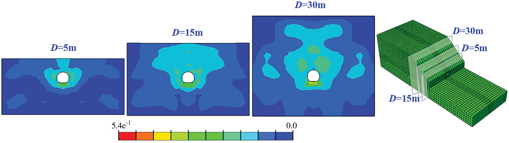
Figure 16: Damage factor contours of rock ground near the tunnel portal under S waves with vibration direction parallel to tunnel axis

The distributions of the strain components at two tunnel cross-sections for S waves with a vibration direction parallel to the tunnel axis are shown in Fig. 18. This figure shows that the tunnel suffers significant hoop shear strain, but only slight hoop axial strain and axial tensile strain. Moreover, the hoop shear strain is much higher around the tunnel haunches than at other positions. This indicates that the tunnel haunches are vulnerable to S waves with a vibration direction parallel to the tunnel axis. The distribution of the hoop shear strain changes at the same pace as the plastic damage at the haunches (see Fig. 17). Fig. 19 plots the distribution of the hoop shear strain at the haunches along the tunnel axis. From Fig. 19, we see that the hoop shear strain increases at first and then decreases with increasing distance from the tunnel entrance, and changes at the same pace as the plastic strain of the tunnel (see Fig. 17).

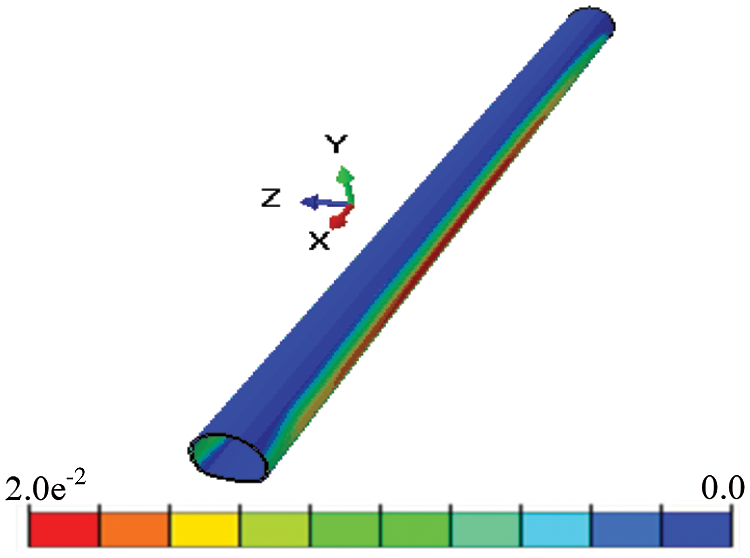
Figure 17: Maximum principal plastic strain contour of tunnel lining under S waves with vibration direction parallel to tunnel axis

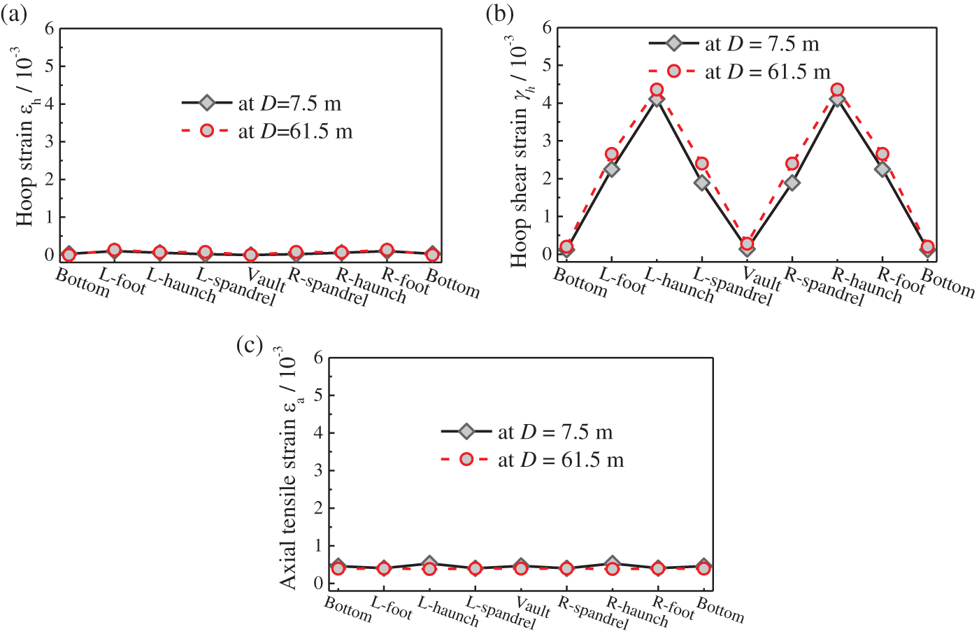
Figure 18: Distribution of strain components along the tunnel cross-sections for S waves with vibration direction parallel to tunnel axis: (a) hoop strain, (b) hoop shear strain, and (c) axial tensile strain

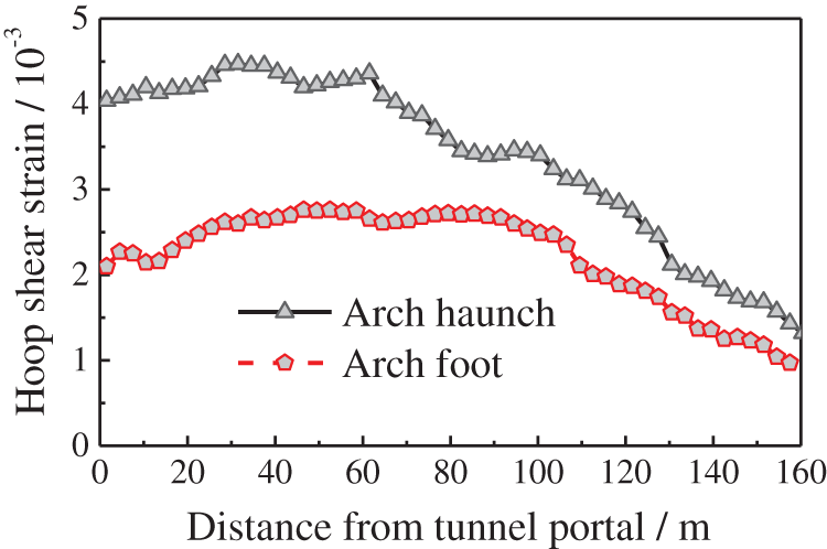
Figure 19: Distribution of hoop shear strain along tunnel axis for S waves with vibration direction parallel to tunnel axis

5.3 Vertically Incident P Waves with Vibration Direction Perpendicular to Tunnel Axis

The seismic response of the tunnel portal under vertically incident P waves with a vibration direction perpendicular to the tunnel axis is now analyzed. The damage factor contours of the rock near the tunnel portal are shown in Fig. 20, and the maximum principal plastic strain contour of the tunnel lining is shown in Fig. 21. The damage contours of the rock, as well as the plastic strain on the tunnel lining, are symmetric and significantly concentrated around the tunnel entrance. With increasing distance from the tunnel entrance, the plastic damage to the tunnel lining quickly decreases. The maximum damage factor of the rock and the maximum plastic strain of the tunnel are significantly lower than in the case of vertically incident S waves.

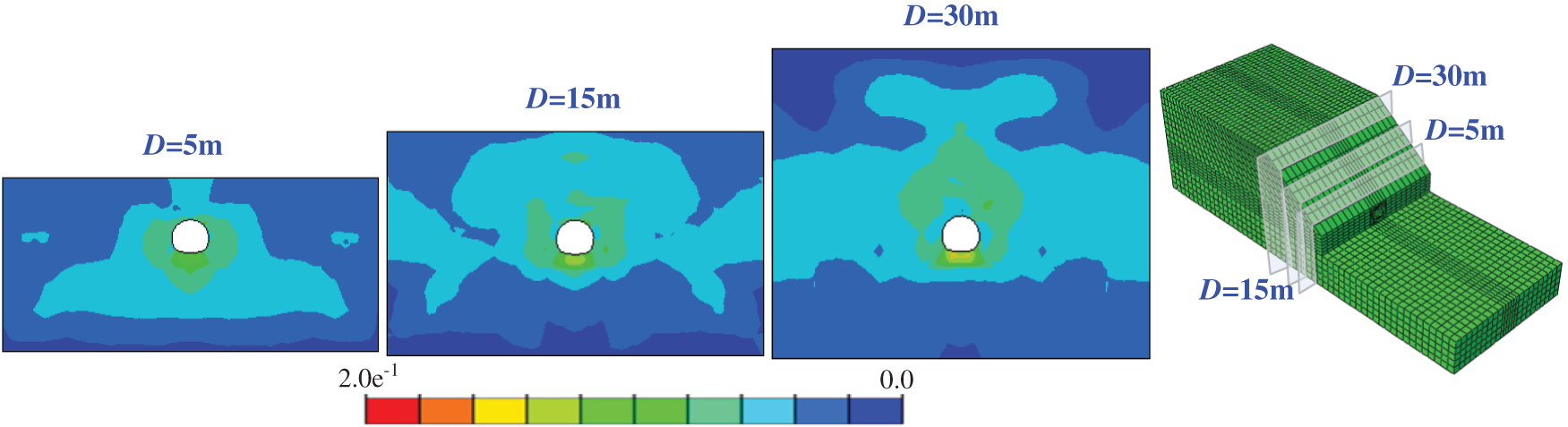
Figure 20: Damage factor contour of rock near the tunnel portal under vertically incident P waves with vibration direction perpendicular to tunnel axis

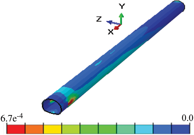
Figure 21: Maximum principal plastic strain contour of the tunnel portal under vertically incident P waves with vibration direction perpendicular to tunnel axis

Fig. 22 shows the distributions of strain components along two tunnel cross-sections for vertically incident P waves. The hoop axial strain εh and hoop shear strain γh are larger than the axial tensile strain εa. Moreover, Fig. 22 indicates that εh and γh are dominant around the tunnel haunches, and change at the same pace as the plastic strain concentrated around the tunnel haunches. Fig. 23 shows the distributions of εh and γh at the tunnel haunches along the tunnel axis. With increasing distance from the tunnel entrance, the hoop axial strain gradually decreases, whereas the hoop shear strain increases at first and then decreases.

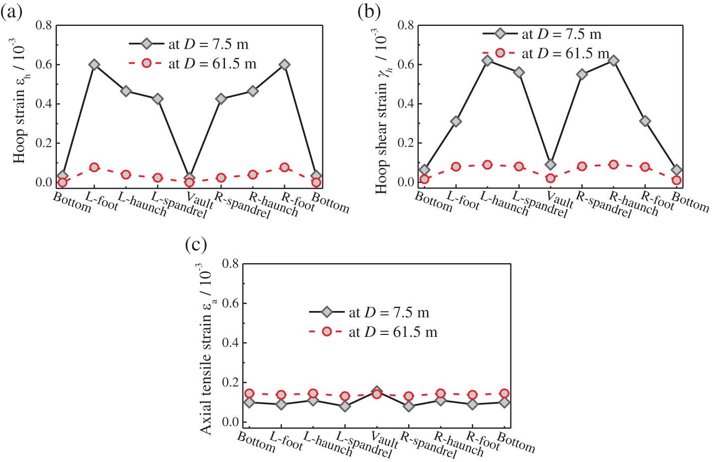
Figure 22: Distributions of strain components along lining cross-sections for vertically incident P waves with vibration direction perpendicular to tunnel axis: (a) hoop strain, (b) hoop shear strain, and (c) axial tensile strain

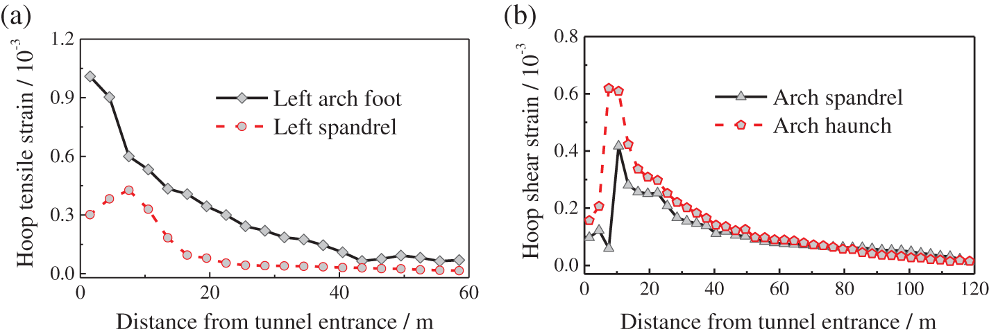
Figure 23: Distributions of strain components along tunnel axis for vertically incident P waves with perpendicular vibration direction: (a) hoop axial strain and (b) hoop shear strain

6  Summary and Conclusions

During past earthquake events, tunnel portals have suffered more serious damage than other tunnel sections. Earthquake waves may propagate in different vibration directions, producing a complex dynamic response in the tunnel portal. Based on the Galongla tunnel project, which is located in a seismic region of China, a 3-D numerical model of the tunnel portal was established to study such effects. The seismic mechanical behavior of the slope rock was simulated using an elastoplastic damage model implemented in ABAQUS through a self-compiled UMAT subroutine. The viscous-spring artificial boundary was used to simulate the radiation damping effect at the truncated boundary. Moreover, a seismic input method for the slope site was established for vertically incident earthquake waves with different vibration directions. The damage characteristics of the Galongla tunnel portal under different vibration directions of earthquake waves were then numerically studied. The conclusions are as follows:

(1)   For vertically incident S waves with a vibration direction perpendicular to the tunnel axis, the hoop tensile strain at the spandrel and arch foot and the hoop shear strain at the vault and arch bottom are the main contributors to the plastic damage of the tunnel. For vertically incident S waves with a vibration direction parallel to the tunnel axis, a very large hoop shear strain occurs at the tunnel haunches. For vertically incident P waves with a vibration direction perpendicular to the tunnel axis, the tunnel is mainly subjected to hoop tensile strain and hoop shear strain.

(2)   The vibration direction of the earthquake waves significantly influences the dynamic response of the tunnel portal. For vertically incident S waves with a vibration direction perpendicular to the tunnel axis, the hoop axial strain at the spandrel and arch foot are dominant at the tunnel entrance, and then rapidly decrease to a stable value away from the tunnel entrance. The hoop shear strain increases at first and then decreases with increasing distance from the tunnel entrance. For vertically incident S waves with a vibration direction parallel to the tunnel axis, the hoop shear strain increases and then decreases with distance from the tunnel entrance. For vertically incident P waves with a vibration direction perpendicular to the tunnel axis, the hoop axial strain decreases gradually, and the hoop shear strain first increases and then decreases with increasing distance from the tunnel entrance.

Acknowledgement: The authors wish to acknowledge financial support from the Beijing Natural Science Foundation Program (JQ19029) and the National Natural Science Foundation of China (41672289; U1839201; 51421005).

Funding Statement: The paper is supported by Beijing Natural Science Foundation Program (JQ19029), and National Natural Science Foundation of China (41672289; U1839201; 51421005).

Conflicts of Interest: The authors declare that they have no conflicts of interest to report regarding the present study.

Appendix

(1)   ∂f∂γp

∂f∂γp=−Mβσ¯1β+σ¯1β+σ¯1β3b1(b1+γp)2(A-1)

(2)   ∂f∂σ¯ij

∂f∂σij=[∂f∂σ11∂f∂σ22∂f∂σ33∂f∂σ12∂f∂σ23∂f∂σ31]=LMN(A-2)

where

L(6,3)=[∂I¯1∂σ¯11∂J¯2∂σ¯11∂J¯3∂σ¯11∂I¯1∂σ¯22∂J¯2∂σ¯22∂J¯3∂σ¯22∂I¯1∂σ¯33∂J¯2∂σ¯33∂J¯3∂σ¯33∂I¯1∂σ¯12∂J¯2∂σ¯12∂J¯3∂σ¯12∂I¯1∂σ¯23∂J¯2∂σ¯23∂J¯3∂σ¯23∂I¯1∂σ¯31∂J¯2∂σ¯31∂J¯3∂σ¯31](A-3)

M(3,3)=[∂σ¯1∂I¯1∂σ¯2∂I¯1∂σ¯3∂I¯1∂σ¯1∂J¯2∂σ¯2∂J¯2∂σ¯3∂J¯2∂σ¯1∂J¯3∂σ¯2∂J¯3∂σ¯3∂J¯3](A-4)

N(3,1)=[∂f∂σ¯1∂f∂σ¯2∂f∂σ¯3]T(A-5)

where

{I¯1=(σ¯11+σ¯22+σ¯33)/3I¯2=σ¯11σ¯22+σ¯22σ¯33+σ¯33+σ¯11−σ¯122−σ¯232−σ¯312I¯3=σ¯11σ¯22σ¯33+2σ¯12σ¯23σ¯31−σ¯11σ¯232−σ¯22σ¯312−σ¯33σ¯122J¯2=(I¯12−3I¯2)/3J¯3=(2I¯13−9I¯1I¯2+27I¯3)/27(A-6)

{σ¯1=I¯13+23J¯2cos⁡θ¯σ¯2=I¯13+23J¯2cos⁡(θ¯−23π)σ¯3=I¯13+23J¯2cos⁡(θ¯+23π)θ¯=13arccos⁡(332J¯3(J¯2)32)(θ¯∈[0,π3])(A-7)

{∂f∂σ¯1=22βσ¯1β−1(2σ¯1β−σ¯2β−σ¯3β)((σ¯1β−σ¯2β)2+(σ¯2β−σ¯3β)2+(σ¯3β−σ¯1β)2)−12−13Mβkβσ¯1β−1∂f∂σ¯2=22βσ¯2β−1(2σ¯2β−σ¯1β−σ¯3β)((σ¯1β−σ¯2β)2+(σ¯2β−σ¯3β)2+(σ¯3β−σ¯1β)2)−12−13Mβkβσ¯2β−1∂f∂σ¯3=22βσ¯3β−1(2σ¯3β−σ¯1β−σ¯2β)((σ¯1β−σ¯2β)2+(σ¯2β−σ¯3β)2+(σ¯3β−σ¯1β)2)−12−13Mβkβσ¯3β−1(A-8)

{∂I¯1∂σ¯11=∂I¯1∂σ¯22=∂I¯1∂σ¯33=1,∂I¯1∂σ¯12=∂I¯1∂σ¯23=∂I¯1∂σ¯31=0∂J¯2∂σ¯11=13(2σ¯11−σ¯22−σ¯33)∂J¯2∂σ¯22=13(2σ¯22−σ¯11−σ¯33)∂J¯2∂σ¯33=13(2σ¯33−σ¯11−σ¯22)∂J¯2∂σ¯12=2σ¯12,∂J¯2∂σ¯23=2σ¯23,∂J¯2∂σ¯31=2σ¯31∂J¯3∂σ¯11=(σ¯22−I¯13)(σ¯33−I¯13)−σ¯232+J¯23∂J¯3∂σ¯22=(σ¯11−I¯13)(σ¯33−I¯13)−σ¯312+J¯23∂J¯3∂σ¯33=(σ¯11−I¯13)(σ¯22−I¯13)−σ¯122+J¯23∂J¯3∂σ¯12=2(σ¯23σ¯31−(σ¯33−I¯13)σ¯12)∂J¯3∂σ¯23=2(σ¯12σ¯31−(σ¯11−I¯13)σ¯23)∂J¯3∂σ¯31=2(σ¯12σ¯23−(σ¯22−I¯13)σ¯31)(A-9)

{∂σ¯1∂I¯1=13,∂σ¯2∂I¯1=13,∂σ¯3∂I¯1=13∂σ¯1∂J¯2=33J¯2−12cos⁡θ¯−32J¯2−2J¯3(1−274J¯2−3J¯32)−12sin⁡θ¯∂σ¯2∂J¯2=33J¯2−12cos⁡(θ¯−23π)−32J¯2−2J¯3(1−274J¯2−3J¯32)−12sin⁡(θ¯−23π)∂σ¯3∂J¯2=33J¯2−12cos⁡(θ¯+23π)−32J¯2−2J¯3(1−274J¯2−3J¯32)−12sin⁡(θ¯+23π)∂σ¯1∂J¯3=J¯2−1(1−274J¯2−3J¯32)−12sin⁡θ¯∂σ¯2∂J¯3=J¯2−1(1−274J¯2−3J¯32)−12sin⁡(θ¯−23π)∂σ¯3∂J¯3=J¯2−1(1−274J¯2−3J¯32)−12sin⁡(θ¯+23π)(A-10)

(3)   ∂g∂σ¯ij

The expression of ∂g∂σ¯ij is similar to that of ∂f∂σ¯ij, just replacing parameter Mβ with Mg.

This work is licensed under a Creative Commons Attribution 4.0 International License, which permits unrestricted use, distribution, and reproduction in any medium, provided the original work is properly cited.