| Computer Modeling in Engineering & Sciences |
DOI: 10.32604/cmes.2022.019245
REVIEW
The Hidden-Layers Topology Analysis of Deep Learning Models in Survey for Forecasting and Generation of the Wind Power and Photovoltaic Energy
1School of Computer, Jiangsu University of Science and Technology, Zhenjiang, 212003, China
2School of Automation, Key Laboratory of Measurement and Control for CSE, Ministry of Education, Southeast University, Nanjing, 210096, China
3School of Information Science and Technology, Nantong University, Nantong, 226019, China
*Corresponding Author: Haijian Shao. Email: jsj_shj@just.edu.cn
Received: 11 September 2021; Accepted: 18 November 2021
Abstract: As wind and photovoltaic energy become more prevalent, the optimization of power systems is becoming increasingly crucial. The current state of research in renewable generation and power forecasting technology, such as wind and photovoltaic power (PV), is described in this paper, with a focus on the ensemble sequential LSTMs approach with optimized hidden-layers topology for short-term multivariable wind power forecasting. The methods for forecasting wind power and PV production. The physical model, statistical learning method, and machine learning approaches based on historical data are all evaluated for the forecasting of wind power and PV production. Moreover, the experiments demonstrated that cloud map identification has a significant impact on PV generation. With a focus on the impact of photovoltaic and wind power generation systems on power grid operation and its causes, this paper summarizes the classification of wind power and PV generation systems, as well as the benefits and drawbacks of PV systems and wind power forecasting methods based on various typologies and analysis methods.
Keywords: Deep learning; wind power forecasting; PV generation and forecasting; hidden-layer information analysis; topology optimization
As the energy crisis, environmental degradation, and climate change worsen, the usage of clean energy is becoming increasingly important. Furthermore, the proportion of wind and photovoltaic energy is growing [1, 2]. Wind and photovoltaic power generation are examples of new energy power generating technologies that are clean, low-carbon, and renewable, which have been widely used in power generation technology. China’s installed power generating capacity reached 2.26 billion kilowatts in June, gaining 9.5 percent year on year, according to statistics issued by the National Energy Administration. The installed solar power capacity was about 270 million kW, up 23.7 percent year on year. Two basic patterns in wind speed are discussed due to the low density of wind energy, atmospheric pressure, humidity, and temperature: on the other hand, wind speed distribution is volatile and has a non-stable random trend. The stability of the output power will be detrimental to power grid dependability, economics, and reduce the uncertainty of wind power due to the randomness of wind and solar power and volatility features [3–5]. Wind power forecasting with high precision is particularly important, and we must successfully carry out power system operation optimization.
To calculate the value of wind power, modeling and mathematical analyses of historical data may be employed. As a consequence, when comparing different forecasting methods, wind speed and wind power may be included in their entirety. Short-term forecasting, or utilizing physical models based on numerical weather predictions and statistical models based on wind speed and wind power data for predicting, is the current trend in wind power forecasting. Artificial intelligence-based wind power forecasting technology has grown in prominence in recent years.
The rest of this paper is organized as follows: The physical model, statistical learning technique, and machine learning method based on historical data are investigated for forecasting wind and solar photovoltaic generation, and the ensemble sequential LSTM approach with optimized Hidden-layers topology for short-term multivariable wind power forecasting is introduced in Section 2; In Section 3, STL (Seasonal-Trend decomposition procedure based on Loess) and the method of SOM cluster is successively applied to decompose the wind power time series into the seasonal and trend component with significant information and optimize the hidden-layer topology of forecasting method. VGG, ResNet and other transfer learning models are used for cloud image classification and the hidden layer feature information of cloud images are used for classification analysis.
2 The Forecasting and Generation Methods of the Wind and Photovoltaic Energy
Large-scale grid-connected power generation is the most effective approach to completely use wind and solar energy due to exposure to sun radiation. The shooting strength, temperature, humidity, cloud volume, and a variety of other parameters, as well as scenic power generation, reveal an inherent follow-up machine and volatility. With the growth of the number of scenic power stations, the demand for real-time monitoring of scenery data has developed. As a result, there is a greater demand for enhanced and safe operation, as well as the ability to evaluate meteorological and landscape data. The survey’s general framework is depicted in Fig. 1. This paper examines the experimental principle, experimental process, experimental results, and sample analysis from the perspective of different classification models in order to find a reliable method to improve the forecasting effect by combining and analyzing the current wind power forecasting system and photovoltaic forecasting system.
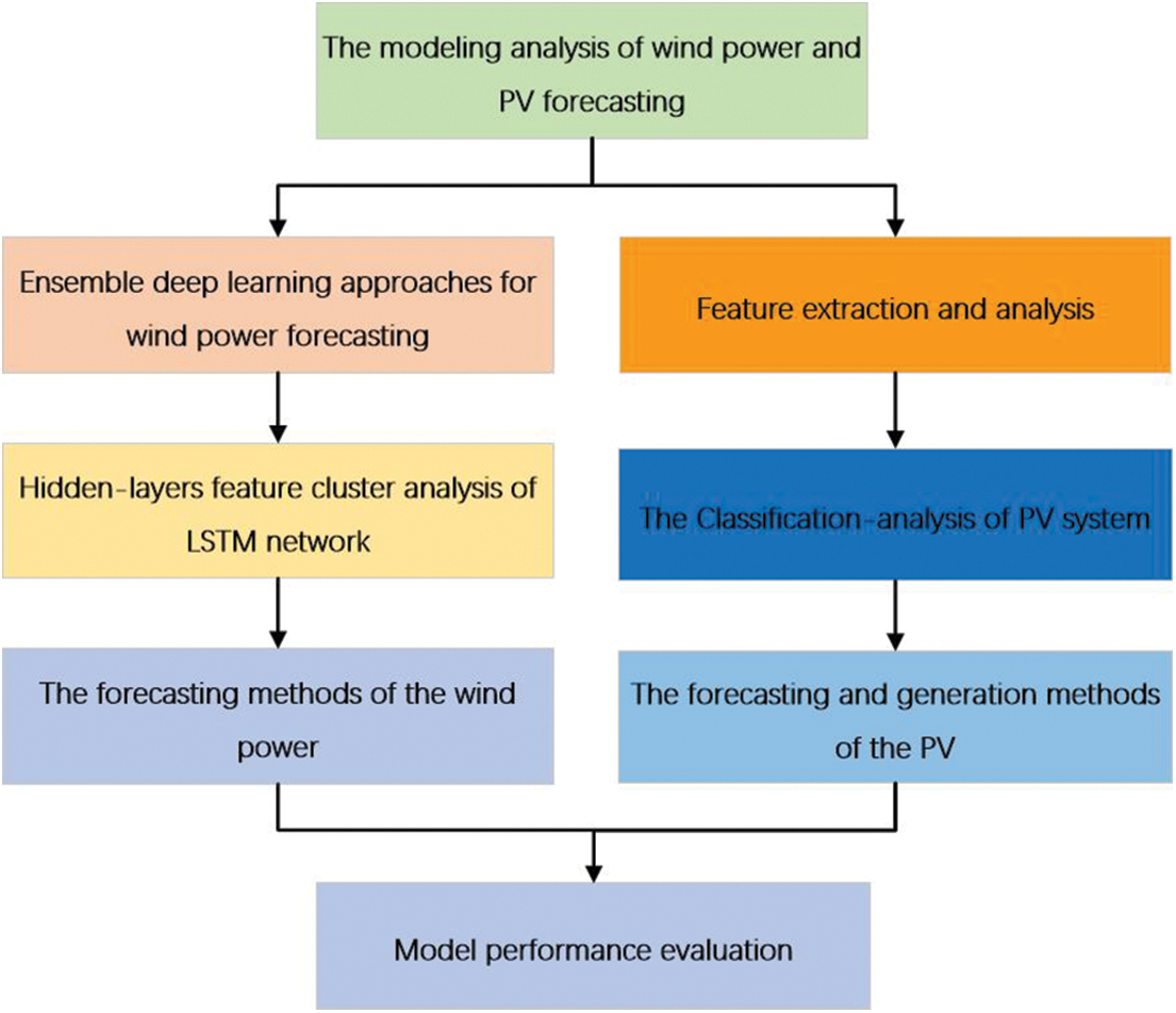
Figure 1: The overall framework of this paper
2.1 The Modeling Analysis of Wind Power Forecasting
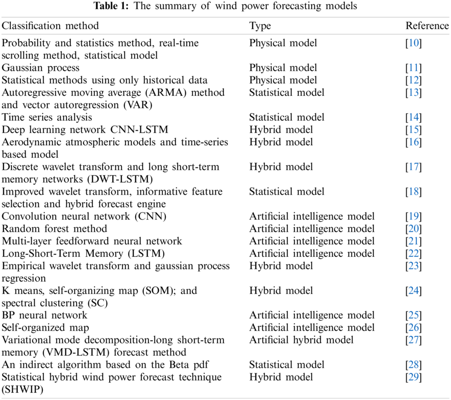
In recent years, the research on wind power forecasting model is very extensive all over the world, and the forecasting methods are also innovating constantly. There are several literatures to summarize the forecasting technology in different development periods of wind power as indicated in Table 1, in order to better apply the existing research results of wind power forecasting technology and improve the forecasting accuracy of wind power forecasting systems. Pinson [6] studied and evaluates various uncertain factors of wind power forecasting accuracy from the aspects of reliability, accuracy and resolution. Zhang et al. [7] highlighted the requirements and overall framework of uncertainty forecasting evaluation by categorizing forecasting approaches into three categories: probabilistic forecasting (parametric and non-parametric), risk index forecasting, and spatiotemporal scenario forecasting. Aggarwal et al. [8], based on NWP, statistical methods, ARIMA models and mixed technologies on different time scales, discussed wind power and important forecasting technologies related to wind speed, and divides the forecasting technologies into statistical models, physical models and mixed models. Foley et al. [9] went into great length about statistical and machine learning methodologies. Benchmarking and uncertainty analysis techniques used for forecasting are outlined and the performance of various methods over different forecast time horizons is examined. The preceding literatures are useful for researching and using wind power forecasting methodologies, as well as improving wind power forecasting accuracy.
In order to establish a more accurate wind power forecasting model, a classification research on wind power forecasting is constructed, which can be summarized as shown in the Fig. 2. According to different forecasting models, wind power forecasting is mainly classified into four categories based on distinct forecasting models: physical model, statistical model, artificial intelligence model, and hybrid model [30–32], and it is classified into ultra-short-term forecast, short-term forecast, medium-term forecast and long-term forecast [33–35] according to different time scales. The wind power forecasting at different time scales:
i) Ultra-short-term forecasting: to forecast the wind power of the next few minutes to a few hours, using the historical data of the wind tower to predict the wind power by continuous method or statistical method, mainly used for the control of wind turbines [36–39].
ii) Short-term forecasting: to forecast the power output in the next few days, often using the method of weather forecast based on data, or using historical data for forecasting, used for reasonable dispatch of the power grid, to ensure the quality of power supply [40–46].
iii) Mid-term forecasting: to forecast the power output in the next few months or weeks, generally using numerical weather forecast methods, mainly used for arranging maintenance of wind farms [47–50].
iv) Long-term forecast: the forecast unit is month or year, which usually requires decades of wind power data to calculate the annual power generation of wind farms, mainly used for feasibility study and site selection of wind farm design [51–55].
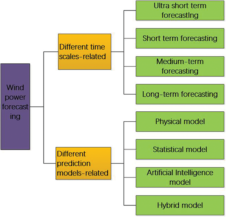
Figure 2: Different classifications of wind power forecasting
2.2 Physical and Statistical Models Related Approaches
The physical model obtains wind speed, wind direction, temperature, and other meteorological data primarily through a numerical weather forecast system (NWP), and then the power curve of a wind turbine is determined by estimating wind speed, yielding the expected power of a wind turbine [10 –12]. NWP is often implemented on supercomputers because it uses high-dimensional and complicated mathematical equations, resulting in significant computational and manpower expenses. As a result, this method’s capacity to foresee in the near term is more broad, and its output is better suited as a long-term reference standard. When observed data is scarce, statistical models must rely on historical wind data, which reduces predicting accuracy. Because actual data is typically random for a variety of reasons, the statistical characteristics of time series change over time. The corresponding mathematical expectation and variance factors will change with time, which will surely make it more difficult to forecast trends based on historical data. Statistical models such as the moving average method [13, 14, 16] and wavelet decomposition [17, 18] have limited ability to predict data with strong nonlinearity due to the random, intermittent, and seasonal changes in wind speed, and statistical models are usually only suitable for short-term forecasting.
2.3 Hybrid Forecasting Modeling Based on Neural Network-Related Approaches
Artificial intelligence models are commonly used in short-term wind power forecasting because of the benefits in dependency analysis and pattern detection [25 –27, 56–60]. Ozkan et al. [61] suggested a multi-feature convolutional neural network-based wind power forecasting approach. To begin, wind power is classed based on the waveform’s changing characteristic. Then, the convolution neural network extracts the feature of the wind power waveform (CNN). The results show that this method can effectively improve the reliability of wind forecasting. Quan et al. [62] put forward the random forest method to construct the wind power predictor before hours, the results show that the proposed model can significantly improve the forecasting accuracy, compared with the classical neural network forecasting. Haque et al. [63] adopted a new recurrent neural network called Long-Short-Term Memory (LSTM), the test results on real data sets show that the performance of LSTM model is better than typical RNN models such as Elman, exogenous nonlinear autoregressive model and other benchmark models.
Despite the stated artificial intelligence models can forecast the short-term wind power [64], the forecasting accuracy is still insufficient. Long-term and short-term memory (LSTM) networks have been widely employed in wind power forecasting because to their capacity to understand the long-distance dependency of time series. The back propagation information may not be extracted in RNN because of the multivariable with long temporal dependency, and the vanish gradient and vanish explosion issues are typically caused in the learning processing of the deep neural networks. By controlling the information updating, the LSTM network can avoid the information exponentially decaying, and effectively overcome the outlined disadvantages of the RNN, as well as improve the forecasting accuracy and robustness of the deep learning [65].
By calculating the vibrational energy distribution for each period, the time series can be viewed of a reconstruction of several periodic disturbances, which is important for identifying the periodic components of the time series [66]. High-accuracy multivariate forecasting modeling remains a challenge due to the varied distributions of time series in different areas. Periodic features may be obtained by decomposing the original time series sequence using a filtering strategy, which can help enhance multivariate time series forecasting and modeling accuracy. Spectral decomposition, wavelet transformation [23 , 67], and time series decomposition models are the most extensively used the approaches of multivariate decomposition. The raw data can be decomposed into trend component, seasonal component, and remaining component using the LOESS-based method of time series decomposition, as illustrated in Fig. 3 [68]. As a result, the forecasting models properly capture the long-term steady trend in timing across time, periodic duration and amplitude fluctuations, as well as irregular changes caused by random factors.
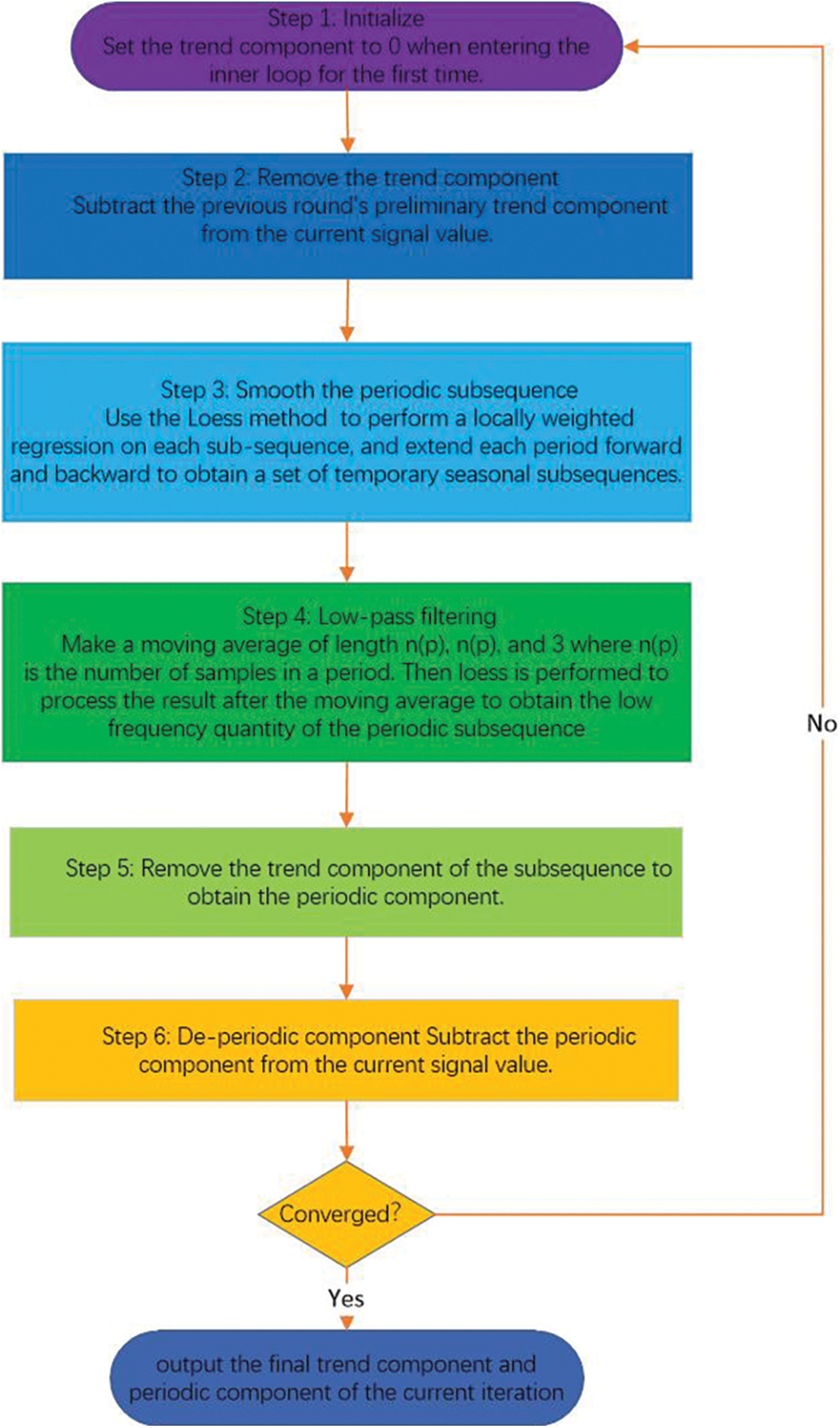
Figure 3: The STL decompresses flow chart
When comparing with a single single method, the weighted combination method can effectively reduce the upper limit of error and improve the robustness of the forecasting results, greatly improving wind speed and wind power forecasting accuracy [15, 19, 20, 22, 24, 69–74]. Neshat et al. [74] utilized a mixture of autoencoder and cluster to decrease the random noise in the original data sequence, then use Variational Mode Decomposition (VMD), Greedy Nelder Mead (GNM) search technique, and Adaptive Randomised Local Search to optimize the hyper-parameters of VMD (ARLS). Finally, a hyper-parameter optimizer combining LSTM and the Self-adaptive Differential Evolution (SaDE) algorithm and sine cosine optimisation approach is employed for modeling. Then Neshat et al. [28] proposed a hybrid model consisting of bidirectional long short-term memory neural network, hierarchical evolutionary decomposition technique and an improved generalised normal distribution optimisation algorithm, the introduced model performed best on average in the two case studies. Shang et al. [29] proposed a comprehensive system of integrated noise reduction, cluster and multi-objective optimization, and its performance in four performance indexes is superior to other comparison models. Jiang et al. [75] presented a four-part combined prediction system that includes optimum sub-model selection, point prediction using a modified multi-objective optimization method, interval forecasting using distribution fitting, and forecasting system assessment. The proposed combined system combines the advantages of the sub-models and gives accurate point and interval forecasting results. The results of the experiments show that the suggested combined forecasting system can produce accurate wind speed point and interval forecasts. A single deep learning model’s forecasting ability may be limited, and the model’s forecasting ability may also be limited due to the influence of subjective experience. Although the deep neural network can capture the descriptive qualities of a sequence with various time delays, the forecasting ability of the network might be improved further by utilizing appropriate data decomposition algorithms to reduce the sequence’s complexity. Ensemble models, in particular, are useful for predicting plausible features and then integrating all of the forecasting results, which helps to increase forecasting model forecasting accuracy and model robustness. Self Organizing Feature Map was introduced to solve the above problems [76]. First, the whole sample is automatically clustered, and then LSTM forecasting models are established according to the similar clustering results. Comparing with other neural networks, LSTM neural network has the advantages of faster budget speed and less difficulty in falling into local minimum points, so LSTM neural network is used for modeling and forecasting of samples [77].
2.4 The Ensemble Deep Learning Approaches for Wind Power Forecasting
The Fourier series principle indicates that any continuous time series or signals can be represented as the superimposing of sine wave signals with different frequencies. Similarly, STL (Seasonal-Trend decomposition procedure based on Loess) can also use the idea of overlays to decompose the time series into complex trends terms, periodic terms and remaining terms [78], which is usually defined by Eq. (1):
where Yt is the input time series, and has three variables Tt, St, and Rt after decomposition. Tt is a trending weight at t-moment, representing the long-term characteristics of the sequence. St is the corresponding periodic variable that represents the periodic characteristics of the sequence. Rt is the remaining item of Yt, which represents the jitter and interference factors that the sequence is subjected to, and is usually considered miscellaneous. One of the most extensively used methods for smoothing discrete data is the Loess (locally weighted scatterplot smoothing) approach. When estimating the value of a response variable, a subset of data is first taken from the region of the target variable, and then linear or quadratic regression is used to this subset. For regression, the weighted least square approach is used, with the weight increasing as it comes closer to the estimation data. Finally, the local regression model is used to estimate the response variable [79, 80]. STL consists of inner loop and outer loop, and the former is mainly used for trend component fitting and periodic component calculation. Through multi-round iteration, the convergence value is utilized to estimate the real value of the probability distribution of the trend and periodic component. In the outer loop, the remainder can be calculated based on the trend component and periodic component obtained in the inner loop. The remainder will not be defined where the input data is missing. Once an outlier is detected, it will produce an abnormality. The outer loop is mainly used to adjust the robustness weight and reduce the size of the remainder for generated outliers [81 , 82].
The ensemble deep learning approaches for wind power forecasting is described in Fig. 4. which is generally made up of four parts: Firstly, the dataset is divided into three groups based on the STL decomposition, trend component, seasonal component and residuals. Usually, the trend and seasonal parts can still show the significant influences to reflect the most the effective information, and the residuals is not a simply white noise, which still has some valid information. However, it has a far smaller impact on sequence predictions than the first two components. This is due to the fact that the render and seasonal components contain the majority of the original sequence’s valid information. Secondly, the data processed by the STL decomposition methods are divided as training sample, validation sample as well as testing sample which are used to train and test the performance of the forecasting models. Thirdly, by the SOM cluster, the hidden-layer information is mapped into the feature space with well sample separation to optimize the hidden topology of LSTM. The precise analysis of the hidden-layers information can reduce the risk caused by over-fitting and improve the robustness of the proposed approaches. Fourthly, the forecasting error is analyzed in mathematical analysis, and the output is constructed by the ensemble LSTM networks. Finally, the benchmarks methods, such as persistence model, multi-SVR, convnets, basic LSTM, cluster LSTM are performed to compare the performance of the proposed approaches, and the forecasting errors are mainly analyzed.
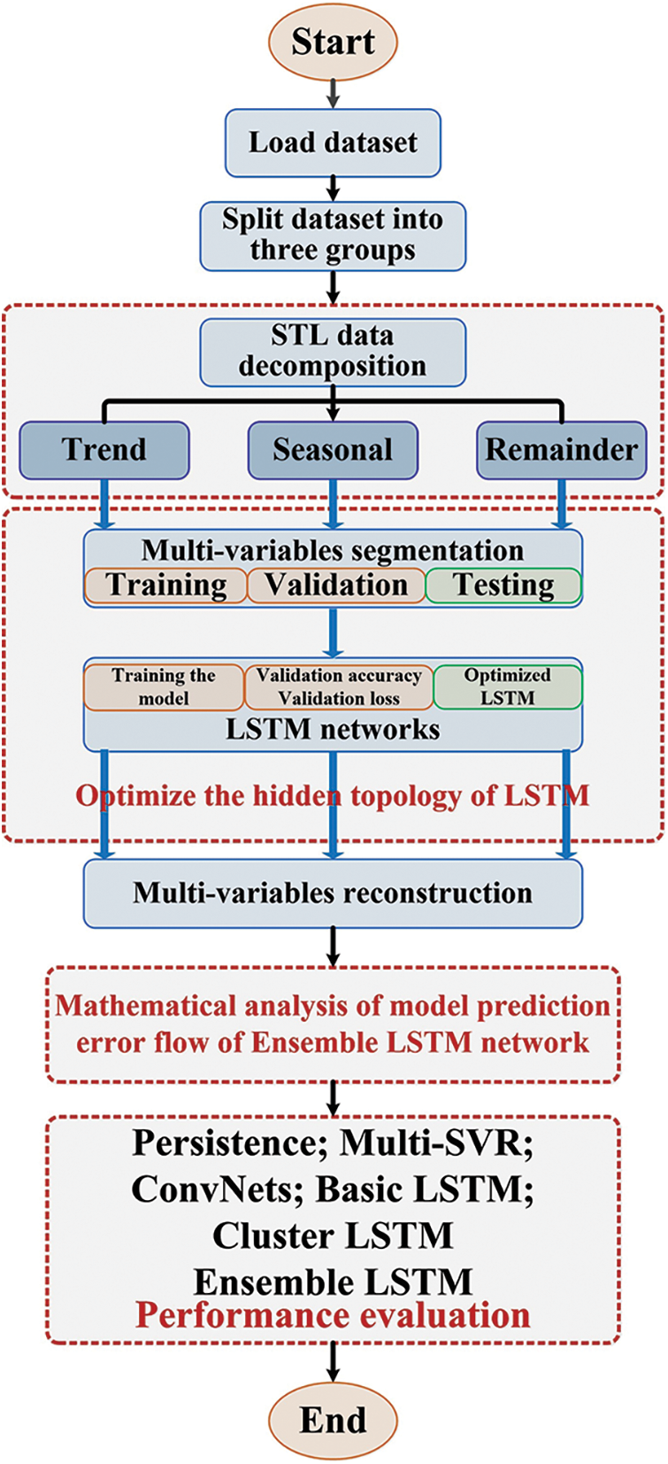
Figure 4: The framework of the multivariable wind power forecasting approaches
2.5 Hidden-Layer Topology Analysis of the LSTM Network
When RNN (Recurrent Neural Network) dealing with ling a long sequence, LSTM network are designed to solve the problem of gradient descent and gradient, as well as overcome short-term dependence. LSTM network can remember the cell state basing on the cell state, and reasonably forget the old state, then add new state and outputting new state [83]. Therefore, the final output ft is given by Eqs. (2)–(4):
The input gate determines that the number of input Xt is retained, and the input is processed by the weight matrix Wc, bias bc, and tanh function. The cell state Ct is given in Eq. (2), and it can be easily seen that a new cell state can be obtained by forgetting part of the past state and adding the existing state based on Eqs. (3) and (4). After multiplying by the cell state Ct, the output gate gets the output Ht of the next stage similar to the forget gate. Eq. (5) is the Ht expression.
Then, the partial derivative between the hidden-states at different times is calculated by Eq. (6):
More precisely, the corresponding gradient is estimated by Eq. (7):
Furthermore, estimating the approximate value of
i.e.,
where
For multipliers in Eq. (10) at any moment, the results can be weighted to be greater than 1 or less than 1. More precisely, the vanishing gradient may be happened when united results became much more smaller. The total product may be larger if the mold of the multiplier at the later moment is greater than 1 through the adjustment of the weight coefficient (i.e., the door). Thus, the long-term memory of time series is preserved. It can be seen from the above that ht has an effect on all errors at the time of
2.6 Hidden-Layers Feature Analysis of LSTM Network
To avoid the infiltration of external information and achieve long-term memory of sequence information, the LSTM network employs a complete structure including forget gates, input gates, and output gates [84, 85]. The LSTM network is commonly used to forecast the future time series output of a single time step in time series. With numerous time steps, an LSTM network can also anticipate the future time sequence output. Multiple variable sequences influence the value of the final variable sequence in a multivariate sequence group. The LSTM model, on the other hand, usually only learns information from a small amount of the time step. Because an interception sequence with a lengthy time step produces low attention value output, the final LSTM network’s predicting impact will be harmed [86 , 87].
The SOM neural network is an unsupervised network that can do unsupervised data grouping [88, 89]. The approach assumes that the input data has certain topological connections or sequences that allow for the realization of the dimensionality reduction mapping from the input n-dimensional space to the output 2-dimensional plane. A typical topological distribution of the input data is then produced on a one-dimensional or two-dimensional processing unit array. The preservation of topological properties resembles the nature of actual brain work. SOM network training adopts the method of “competitive learning” [90, 91]. Each input sample finds a node with the shortest distance from it in the output layer, that is, the most matching node, which is called activation node or winning unit. Then, the node’s parameters are then updated using the stochastic gradient descent approach. At the same time, the points adjacent to the activated node also update their parameters appropriately according to their distance from the activated node [92 –94].
When designing the SOM network, we must take into account the number of neurons in the output layer [95–97]. The number of neurons in the out-put layer is related to the final number of clusters. More neurons can be set to better map the topological structure of the sample in the case of unknowing the number of clusters. If the number of clusters is too large, the output nodes can be appropriately reduced. Therefore, when dividing and selecting ‘regions’ in the clustering plane, the “distance” between samples can be calculated and then the potential categories of different hidden-layer features can be analyzed basing on the similarity measurement between different hidden-layer information. The corresponding distance formula is obtained according to Eq. (11):
where a, b is two arbitrary information points on a two-dimensional plane, the above formula indicates that the closer the hidden layer information is, the more similar the two sample patterns are. In particularly, the patterns of the two samples are the same if the distance obtained by Eq. (11) between the information patterns is zero. In the cluster analysis of the hidden-layer information, the presented threshold is usually used to judge whether the hidden-layer information between different samples is considered as the same, or will be treated in different categories [98 , 99].
2.7 The Forecasting and Generation Methods of the PV System
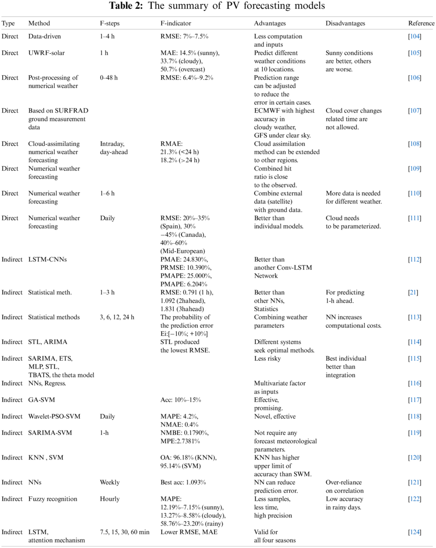
As indicated in Table 2, there are two types of photovoltaic power forecasting methods: direct forecasting based on a physical model and indirect forecasting based on historical data [100–103]. The direct forecasting methods relies heavily on weather values or weather cloud maps, as well as other data, to predict energy generation [104–111], Ground cloud map model [112], a forecasting model integrating weather values with cloud cover pictures [21], and so on. The direct forecasting approach necessitates precise weather prediction information, power station geography information, and a considerable amount of sky picture information, as well as stringent gathering equipment and methods, resulting in the forecasting method’s weak resilience. Simultaneously, the model utilized in the direct forecasting technique is unable to gather time correlation information and is incapable of recalling past data. Indirect forecasting methods include time series method [113–116], Regression analysis [117] and artificial intelligence methods such as artificial neural network [118–125]. The indirect forecasting method can overcome the difficulties such as the lack of physical mechanism of the direct forecasting method, which is suitable for short-term and ultra-short-term photovoltaic power forecasting, as well as long-term and short-term memory [126–128].
Due to the blocking of solar radiation by moving clouds, the photovoltaic power fluctuates rapidly and dramatically in minutes, posing a significant threat to the power grid’s reliability [129–132]. The traditional photovoltaic power forecasting model based on the historical power data of photovoltaic power stations and numerical weather forecast is restricted by the algorithm principle and data accuracy, and it is difficult to precisely predict the minute power fluctuation caused by cloud movement [133–136]. However, under certain weather conditions such as overcast, the surface irradiance fluctuates dramatically in minute time scale because of the influence of moving clouds [137–141]. At this time, there is almost no correlation between the irradiance fluctuation and the historical irradiance data [142, 143]. Therefore, the above phenomena pose a challenge to the extraction and forecasting of minute level meteorological features.
Zhen et al. [144] took pictures of clouds in the sky with the all-sky imager to obtain the visual cloud features, and on this basis, predicts the ultra-short-term photovoltaic power [145]. Zhen et al. [146] proposed a computing method for cloud motion velocity of solar photovoltaic power forecasting (PCPOW) sky image based on pattern classification and particle swarm optimization weight, and simulates it using real data recorded by Yunnan Electric Power Research Institute. The results confirme that PCPOW can improve the accuracy of displacement calculation. Cros et al. [147] proposed a forecasting method based on phase correlation algorithm for motion estimation between subsequent nebula-images derived from Meteosat-9 images. The forecasting of this method is 21% better than the relative RMSE persistence of the cloud index. It is found that sky images are widely used to improve weather forecast performance [148, 149], and cloud identification is one of the challenges faced by photovoltaic forecasting.
The neural network is an artificial intelligence system model that models and links the basic unit neurons of the human brain to replicate the activities of the human brain neuron system selection, pattern recognition, correlation analysis, and learning. The network learning algorithm performs network training by constantly altering the learning rate and weight of the network neuron nodes, and the model can design the learning environment using the input data samples or patterns. The training results will be dispersed across the neuron nodes that were first built. After repeated training analysis, the weight of network neuron nodes will approach a predefined value. Finally, the network can classify data samples autonomously and select the obvious qualities after learning and training.
3.1 The Short-Term Wind Power Forecasting Based on the Hidden-Layers Topology Analysis
The Kohonen neural network is a common unsupervised learning technique, whose network structure and learning algorithms have a better feature selection ability than other neural networks. In the learning or training stage, the Kohonen network structure-based clustering algorithm can adapt to the learning environment, adjust and optimize the learning rate and neuron weight, receive external data samples and environmental characteristics as input, as well as divide different categories of regions autonomously. In Fig. 6, SOM analyzes the hidden layer information of the deep neural network, reduces the dimension and maps the read hidden layer information into the two-dimensional space. The first line of Fig. 6 delicate, before the STL data decomposition, the number of clusters is not obvious, that is, the geometric relationship between clusters or the nodes that can be used as clusters in the topology are not obvious. The corresponding error trend fluctuates sharply around the peak value, which indicats that the convergence speed of the algorithm at this time will be affected by the local area of the data.
The second row to the fourth row of Fig. 5, and display the data trend, cycle, and residual items into low dimensional discrete data, the network nodes are mapped to the local area and the active point in the network. After Competitive Process, Cooperation Process and Adaptation Process, the low dimensional data clustering center of the respectively show about 1 2. The attenuation of vector corresponding with the time of learning, as well as the convergence speed of SOM have the effect of reducing, and the corresponding error is reduced gradually.
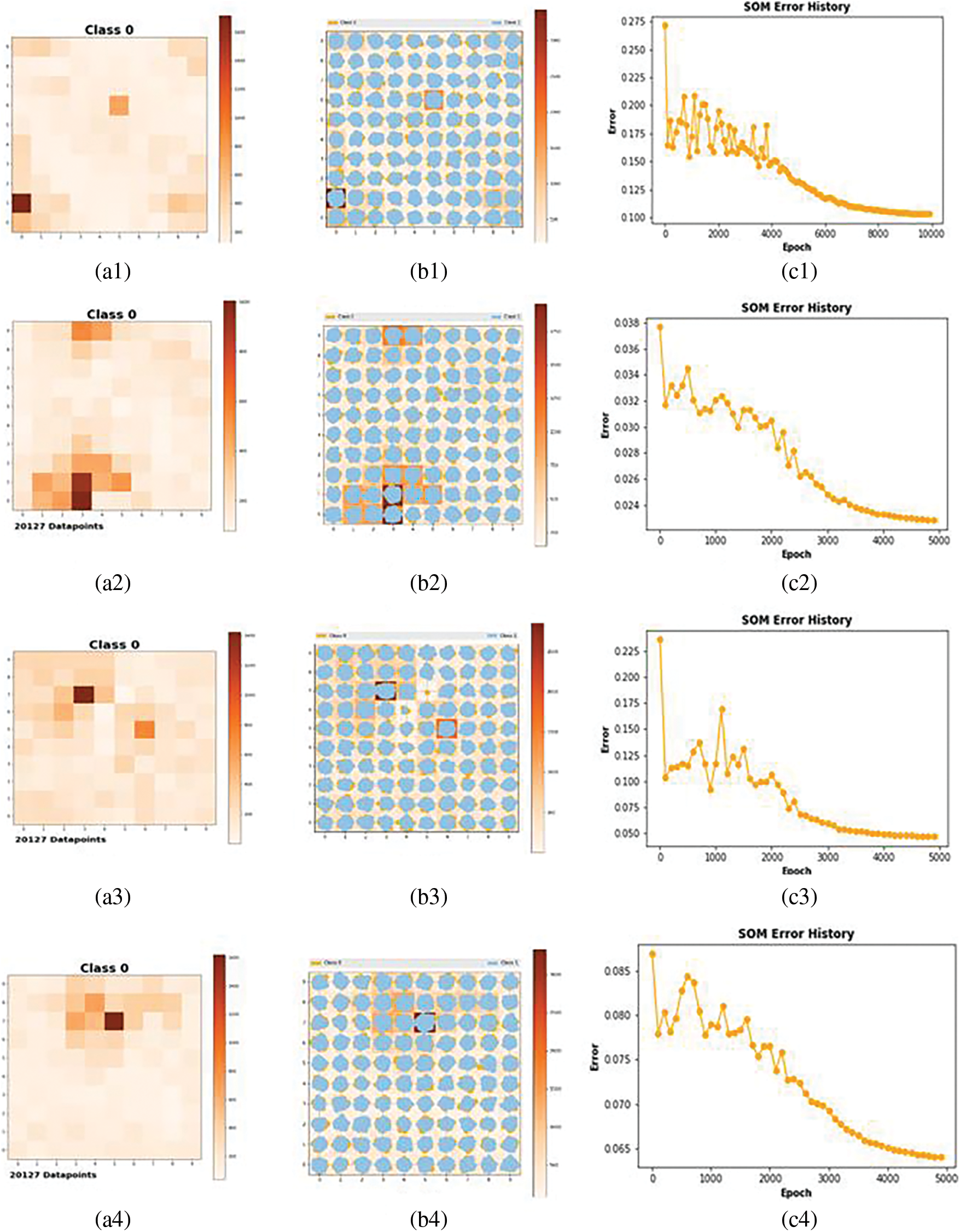
Figure 5: The hidden layer information of the deep neural network: cluster visualization and som error history
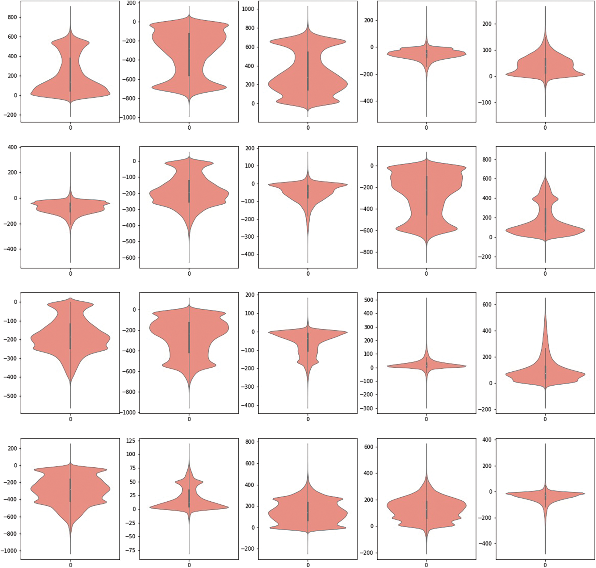
Figure 6: The hidden layer information of the deep neural network in different neurons
Designing the number of hidden nodes requires to read the information of the hidden layer. There are 40,254 pieces of output dable by LSTM, and the feature value dimension of the sample data at each time point is 20. The following Fig. 6 shows the violin chart of the data feature value, which shows the distribution and probability density of the data. The thick black bar in the middle of the violin chart is used to show the quartile, the white dot in the middle of the black thick bar represents the median. The top and bottom edges of the thick bar represent the upper quartile and the lower quartile, respectively. The value of the quartile can be seen from the value of the y-axis corresponding to the position of the edge can see the value of the quartile. The two sides of the graph reflect the density information of the data. The data density at any position can be seen from the shape of the violin graph, the feature distribution of the time series more intuitively is estimated. From the previous analysis of the hidden layer information, it can be seen that the closer the hidden layer information is, the more similar the two sample patterns are, and they can be classified into the same category. Therefore, the 20 hidden layer nodes can be reduced to 6.
For the proportion of places inhabited by a given sample of the cluster, the associated accuracy can be shown as a percentage of the map’s logarithmic sample response, or computed as a percentage of the data sample’s response on the map. BMU is the closest representation of the data sample to the above percentages, estimating accuracy through relative quantization errors and fuzzy responses (quantitative nonlinear functions and percentages of all map units). The quantitative results were analyzed by displaying a histogram (or aggregate response). In fact, if treating the data result as a table shape, a cylinder or ring graph can be visualized, and the map shapes containing flat visualization percentages also will be visualized by using self-organizing grid graphics. The statistical results show that the average algorithm quantization error of trend term, period term and residual term after original data, and STL data decomposition is 0.175, 0.032, 0.125 and 0.080. Comparing with the hidden layer characteristic analysis of the original data, the average fluctuation degree of the data characteristic after STL decomposition is reduced by about 54.85%. According to the above analysis, the number of hidden layer nodes is reduced from the original artificial experience of 20 (related to the number of inputs, which are determined by the order of the model) to 68. Thus, the preliminary optimization of hidden layer topology structure of deep LSTM network is designed.
When evaluating the prediction capacity of time series models, it is critical to use the baseline model. In general, the baseline model is easy to implement forecasting modeling and naive of problems-specific details. For example, the persistence model can quickly, simply and repeatable calculate the corresponding expected output based on the current input, so as to effectively measure the reliability and effectiveness of the forecasting model currently established [150–157]. Multiple vector regression analysis (Multi-SVR) is a common kind of time-series forecasting model, which can use statistical methods to determine the quantitative relationship of the interdependence between multiple variables [158–160]. Especially the modeling of causal forecasting in the big data, Multi-SVR is used to establish the forecasting model with high accuracy, and mainly used in the model to determine the development regularity of time series data [161–164]. CNN has the analysis ability of using the convolution kernel feature analysis, especially the hidden layer’s awareness of the deep network information [165–169]. Through the establishment of a strong expression ability of nonlinear mapping, it can effectively and accurately analyze data and on the basis of the law of the development trend of the current data, and speculated the data law of development in the future [170–172].
The LSTM network works well for evaluating and forecasting important events in time series with long gaps and delays, which have a improved classification accuracy and parallel processing power, as well as the ability to properly discern the trend development between historical data and anticipated variables. However, several factors in this model must be tweaked, particularly the calculation of topology structure, weight, and hidden-layer threshold. If the hidden-layer data cannot be adequately comprehended. In other words, accurate analysis of the deep neural network’s hidden-layer information is beneficial to the model’s generalization capacity. Furthermore, ensemble LSTM approaches can combine many trained LSTM models and increase each LSTM model’s learning ability, resulting in better and more reliable outputs.
Table 3 shows that the ensemble LSTM model has a greater forecasting accuracy than Persistence, Multi-SVR, ConvNets, Basic LSTM and Cluster LSTM, in every step in the next hour. The improvement of model accuracy also shows that memory gate and forgetting gate in LSTM network structure have significant advantages in dealing with long history dependence. More ever, When the method of SOM cluster is applied to wind power forecasting, it can provide guidance for wind power operation and dispatch. Compared with the traditional LSTM network, the forecasting accuracy of the Ensemble LSTM has been respectively improved by 44.51%, 41.90%, 41.89%, 41.39%, 38.83% and 9.42%. The detailed forecasting results are given in Table 4.
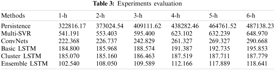
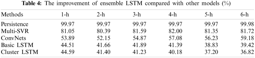
Comparing with the benchmark model such as Persistence, Multi-SVR, ConvNets, Basic LSTM and Cluster LSTM, the forecasting accuracy has been improved by (1-h ahead) 99.97%, 81.05%, 53.89%, 44.51% and 44.59%, (2-h ahead) 99.97%, 80.39%, 52.15%, 41.66% and 41.40%, (3-h ahead) 99.97%, 81.59%, 54.87%, 41.89% and 41.23%, (4-h ahead) 99.97%, 82.00%, 57.08%, 41.39% and 40.18%, (5-h ahead) 99.97%, 81.35%, 56.23%, 38.83% and 37.20%, (6-h ahead) 99.98%, 81.72%, 59.18%, 39.42% and 36.82%. Compared to the traditional LSTM network, the forecasting accuracy of the Ensemble LSTM has been respectively improved by 44.51%, 41.90%, 41.89%, 41.39%, 38.83% and 9.42%. The detailed forecasting results are given in Tables 3 and 4. It can be seen that, no matter what dataset it is, CNNs based on the new topology gets the highest accuracy. On the MNIST dataset, CNNs based on the improved topology has no obvious advantages and achieves an average accuracy improvement of 7%. However, the accuracy in other datasets has improved by 30% and 7%, which achieves a great advance of the topology-optimized network.
3.2 The PV Classification and Forecasting Based on the Hidden-Layers Topology Analysis
Although the bulk of cloud identification depends on visual observation by meteorological observers, the majority of manual identification conclusions are likely to be incorrect depending on the observers’ competence and physical state [173–175]. Furthermore, continuous long-term observation is not practicable owing to the diversity of cloud morphologies and the difficulties of manual observation, affecting cloud identification accuracy and consistency [176–178]. Intelligent cloud categorization and recognition technology has become a prominent study area in meteorology in recent years, thanks to the rapid growth of digital image processing technology. Satellite cloud image research has a wide range and span, but the description accuracy of high resolution and local cloud information is not very good, whereas ground-based cloud image classification has the advantages of ease of operation and strong local guidance, which is something that researchers are concerned about [179, 180]. The multi-category support vector machine (MSVM) is employed in the literature [181] for cloud classification of satellite radiation data, demonstrating MSVM’s promise as a cloud detection and classification system. A classification technique based on extreme learning machines and K nearest neighbors is suggested in the literature [182]. Simulation results show that the proposed model is more suitable for cloud classification than extreme learning machine (ELM) model and artificial neural network (ANN) model. Reference [183] develops a novel time update method for a probabilistic neural network (PNN) classifier to track time changes in image sequences. The results on satellite cloud image data show that the classification accuracy of this method is improved. In literature [184], the fuzzy set algorithm is used for cloud classification of satellite data. Through careful analysis of the fuzzy set, spectral channels are most suitable for the information of specific feature classification are determined. The feature extraction network architecture of nephogram is shown in Fig. 7.
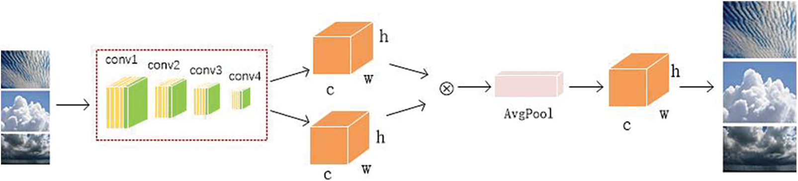
Figure 7: The model structure for feature extraction
CNN has a great capacity to extract visual features and has been used in the categorization of cloud images [133]. At present, in the field of deep learning, such as VGG16 [185–187], ResNet [188–191] and InceptionResnet-v2 [192–195]. CNN have achieved good results in classification, so these mature research results can be used as a reference cloud classification model can be built [196, 197]. In order to guarantee higher accuracy, shown in the following Table 5, this paper tests the five classical model: VGG16, ResNet18, ResNet34, ResNet50, InceptionResnnetv2 migration learning accuracy, and compared with ordinary CNN, found that ordinary CNN has the highest accuracy, at 0.8. This is because, while deeper hidden layers in deep neural networks may extract characteristics with better resolution, the model is also easier to overfit [198–201]. Fig. 8 shows the information of the first four hidden layers of the cloud image data set. It can be seen that the texture features of the cloud image in the first three layers are well retained. The fourth layer begins to learn invalid features. In order to further the cloud, a rich hierarchy of objects for feature extraction, a kind of attention mechanism making the model more focus on the characteristics of effective figure is designed. In the structure, two tensors of extended channel dimensions are firstly used to obtain features, and average pooling and max pooling are performed respectively. The former for spatial information aggregation, which can extract the texture information of the object, be able to infer updated channel information. Then, the output feature vectors are multiplied to connect the two channels, and finally the overall feature extraction of the connected channels is carried out through the two fully connected layers. The accuracy rate was finally reached 92%.
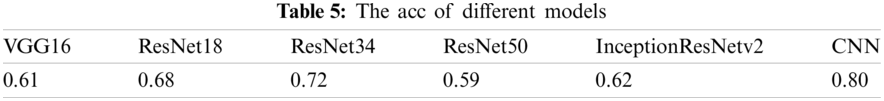
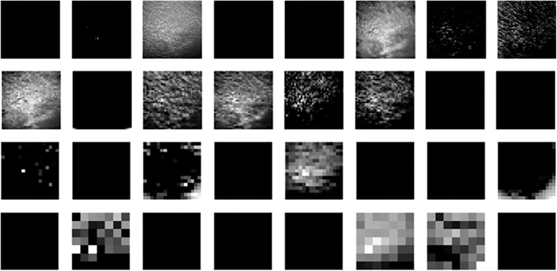
Figure 8: The hidden layer information of CNN for cloud cover
Wind power and solar power generation are widely employed in the power grid, and power system optimization is becoming increasingly important. In this paper, Firstly, the physical model, statistical model, and machine learning model for wind power forecasting are fully detailed, and the hybrid machine learning method is universal and effective, especially in short-term wind power forecasting. Secondly, the set order LSTMs method based on optimized hidden layer topology is emphatically introduced, which is utilized for short-term multivariable wind power forecasting. The STL is used to obtain the trend component, seasonal component and residuals, to reflect the most effective information for short-term wind power forecasting. And the hidden-layer information is mapped into a higher-dimensional feature space, so that the similar information of hidden-layer are well separated via the SOM clusters. The forecasting error of the ensemble LSTM network is analyzed in mathematical analysis. Thirdly, we summarizes the direct method based on physical model and the indirect method based on historical data in photovoltaic power generation forecasting, emphasiz the importance of cloud map identification photovoltaic power generation forecasting. Finally, the performance of the ensemble deep learning approaches is compared to benchmark methods such as persistent model, multi-support vector machine, convolution, basic LSTM and cluster LSTM, and the forecasting error is thoroughly examined. The accuracy of cloud image classification is compared to VGG16, ResNet18, ResNet34, ResNet50, InceptionResNetv2, CNN and other benchmark methods, and the hidden layer feature information of the model is emphatically analyzed. Through our research, it is found that wind power prediction and photovoltaic prediction have similar characteristics. Solar radiation, wind speed and cloud change are all important factors affecting the two kinds of power generation. Therefore, in order to improve the accuracy of prediction, it is the trend for future power generation prediction to extract predicted time characteristics from multiple factors.
Acknowledgement: Thanks the editors of this journal and the anonymous reviewer.
Funding Statement: This project is supported by the National Natural Science Foundation of China (NSFC) (Nos. 61806087, 61902158).
Conflicts of Interest: The authors declare that they have no conflicts of interest to report regarding the present study.
1. Zheng, Z., Chen, Y., Huo, M., Zhao, B. (2011). An overview: The development of prediction technology of wind and photovoltaic power generation. Energy Procedia, 12, 601–608. DOI 10.1016/j.egypro.2011.10.081. [Google Scholar] [CrossRef]
2. Deng, X., Shao, H., Hu, C., Jiang, D., Jiang, Y. (2020). Wind power forecasting methods based on deep learning: A survey. Computer Modeling in Engineering & Sciences, 122(1), 273. DOI 10.32604/cmes.2020.08768. [Google Scholar] [CrossRef]
3. Vargas, S. A., Esteves, G. R. T., Maçaira, P. M., Bastos, B. Q., Oliveira, F. L. C. et al. (2019). Wind power generation: A review and a research agenda. Journal of Cleaner Production, 218, 850–870. [Google Scholar]
4. Wang, X., Guo, P., Huang, X. (2011). A review of wind power forecasting models. Energy Procedia, 12, 770–778. DOI 10.1016/j.egypro.2011.10.103. [Google Scholar] [CrossRef]
5. Das, U. K., Tey, K. S., Seyedmahmoudian, M., Mekhilef, S., Idris, M. Y. I. et al. (2018). Forecasting of photovoltaic power generation and model optimization: A review. Renewable and Sustainable Energy Reviews, 81, 912–928. DOI 10.1016/j.rser.2017.08.017. [Google Scholar] [CrossRef]
6. Pinson, P. (2006). Estimation of the uncertainty in wind power forecasting (Ph.D. Thesis). École Nationale Supérieure des Mines de Paris. [Google Scholar]
7. Zhang, Y., Wang, J., Wang, X. (2014). Review on probabilistic forecasting of wind power generation. Renewable and Sustainable Energy Reviews, 32, 255–270. DOI 10.1016/j.rser.2014.01.033. [Google Scholar] [CrossRef]
8. Aggarwal, S. K., Gupta, M. (2013). Wind power forecasting: A review of statistical models-wind power forecasting. International Journal of Energy Science, 3(1), 1–10. [Google Scholar]
9. Foley, A. M., Leahy, P. G., Marvuglia, A., McKeogh, E. J. (2012). Current methods and advances in forecasting of wind power generation. Renewable Energy, 37(1), 1–8. DOI 10.1016/j.renene.2011.05.033. [Google Scholar] [CrossRef]
10. Chunyan, L., Qin, C., Lili, W. (2015). Wind-storage coupling based on actual data and fuzzy control in multiple time scales for real-time rolling smoothing of fluctuation. Electric Power Automation Equipment, 35(2), 35–41. DOI 10.16081/j.issn.1006-6047.2015.02.006. [Google Scholar] [CrossRef]
11. Fang, S., Chiang, H. D. (2016). A high-accuracy wind power forecasting model. IEEE Transactions on Power Systems, 32(2), 1589–1590. DOI 10.1109/TPWRS.2016.2574700. [Google Scholar] [CrossRef]
12. Qian, Z., Pei, Y., Cao, L., Wang, J., Jing, B. (2016). Review of wind power forecasting method. High Voltage Engineering, 42(4), 1047–1060. [Google Scholar]
13. Erdem, E., Shi, J. (2011). Arma based approaches for forecasting the tuple of wind speed and direction. Applied Energy, 88(4), 1405–1414. DOI 10.1016/j.apenergy.2010.10.031. [Google Scholar] [CrossRef]
14. Sfetsos, A. (2002). A novel approach for the forecasting of mean hourly wind speed time series. Renewable Energy, 27(2), 163–174. DOI 10.1016/S0960-1481(01)00193-8. [Google Scholar] [CrossRef]
15. Kuang, H., Guo, Q., Li, S., Zhong, H. (2021). Short-term wind power forecasting model based on multi-feature extraction and CNN-LSTM. IOP Conference Series: Earth and Environmental Science, vol. 702. Shenzhen, China, IOP Publishing. DOI 10.1088/1755-1315/702/1/012019. [Google Scholar] [CrossRef]
16. Eldali, F. A., Hansen, T. M., Suryanarayanan, S., Chong, E. K. (2016). Employing arima models to improve wind power forecasts: A case study in ercot. North American Power Symposium, Denver, CO, USA, IEEE. DOI 10.1109/NAPS.2016.7747861. [Google Scholar] [CrossRef]
17. Liu, Y., Guan, L., Hou, C., Han, H., Liu, Z. et al. (2019). Wind power short-term prediction based on LSTM and discrete wavelet transform. Applied Sciences, 9(6), 1108. DOI 10.3390/app9061108. [Google Scholar] [CrossRef]
18. Liu, Z., Hajiali, M., Torabi, A., Ahmadi, B., Simoes, R. (2018). Novel forecasting model based on improved wavelet transform, informative feature selection, and hybrid support vector machine on wind power forecasting. Journal of Ambient Intelligence and Humanized Computing, 9(6), 1919–1931. DOI 10.1007/s12652-018-0886-0. [Google Scholar] [CrossRef]
19. Huang, Q., Wang, H. (2020). Wind power forecast based on convolutional neural network with multi-feature fusion. Journal of Physics: Conference Series, 1684. DOI 10.1088/1742-6596/1684/1/012134. [Google Scholar] [CrossRef]
20. Lahouar, A., Slama, J. B. H. (2017). Hour-ahead wind power forecast based on random forests. Renewable Energy, 109, 529–541. DOI 10.1016/j.renene.2017.03.064. [Google Scholar] [CrossRef]
21. Khosravi, A., Machado, L., Nunes, R. (2018). Time-series prediction of wind speed using machine learning algorithms: A case study osorio wind farm, Brazil. Applied Energy, 224, 550–566. DOI 10.1016/j.apenergy.2018.05.043. [Google Scholar] [CrossRef]
22. Duan, J., Wang, P., Ma, W., Tian, X., Fang, S. et al. (2021). Short-term wind power forecasting using the hybrid model of improved variational mode decomposition and correntropy long short-term memory neural network. Energy, 214, 118980. DOI 10.1016/j.energy.2020.118980. [Google Scholar] [CrossRef]
23. Shao, H., Deng, X. (2018). AdaBoosting neural network for short-term wind speed forecasting based on seasonal characteristics analysis and lag space estimation. Computer Modeling in Engineering & Sciences, 114(3), 277–293. DOI 10.3970/cmes.2018.114.277. [Google Scholar] [CrossRef]
24. Shi, J., Ding, Z., Lee, W. J., Yang, Y., Liu, Y. et al. (2013). Hybrid forecasting model for very-short term wind power forecasting based on grey relational analysis and wind speed distribution features. IEEE Transactions on Smart Grid, 5(1), 521–526. DOI 10.1109/TSG.2013.2283269. [Google Scholar] [CrossRef]
25. Wang, S., Liu, X., Jin, Y., Qu, K. (2015). A short term forecasting method for wind power generation system based on BP neural networks. Advanced Science and Technology Letters, 83, 71–75. DOI 10.14257/astl.2015.83.14. [Google Scholar] [CrossRef]
26. Sideratos, G., Hatziargyriou, N. D. (2007). An advanced statistical method for wind power forecasting. IEEE Transactions on Power Systems, 22(1), 258–265. DOI 10.1109/TPWRS.2006.889078. [Google Scholar] [CrossRef]
27. Alexiadis, M., Dokopoulos, P., Sahsamanoglou, H., Manousaridis, I. (1998). Short-term forecasting of wind speed and related electrical power. Solar Energy, 63(1), 61–68. DOI 10.1016/S0038-092X(98)00032-2. [Google Scholar] [CrossRef]
28. Sideratos, G., Hatziargyriou, N. D. (2007). An advanced statistical method for wind power forecasting. IEEE Transactions on Power Systems, 22(1), 258–265. DOI 10.1016/j.enconman.2021.114002. [Google Scholar] [CrossRef]
29. Alexiadis, M., Dokopoulos, P., Sahsamanoglou, H., Manousaridis, I. (1998). Short-term forecasting of wind speed and related electrical power. Solar Energy, 63(1), 61–68. DOI 10.1016/j.energy.2021.122024. [Google Scholar] [CrossRef]
30. Soman, S. S., Zareipour, H., Malik, O., Mandal, P. (2010). A review of wind power and wind speed forecasting methods with different time horizons. North American Power Symposium 2010, Arlington, TX, USA, IEEE. [Google Scholar]
31. Costa, A., Crespo, A., Navarro, J., Lizcano, G., Madsen, H. et al. (2008). A review on the young history of the wind power short-term prediction. Renewable and Sustainable Energy Reviews, 12(6), 1725–1744. DOI 10.1016/j.rser.2007.01.015. [Google Scholar] [CrossRef]
32. Wang, J., Song, Y., Liu, F., Hou, R. (2016). Analysis and application of forecasting models in wind power integration: A review of multi-step-ahead wind speed forecasting models. Renewable and Sustainable Energy Reviews, 60, 960–981. DOI 10.1016/j.rser.2016.01.114. [Google Scholar] [CrossRef]
33. Chandra, D. R., Kumari, M. S., Sydulu, M. (2013). A detailed literature review on wind forecasting. International Conference on Power, Energy and Control, Dindigul, India, IEEE. [Google Scholar]
34. Colak, I., Sagiroglu, S., Yesilbudak, M. (2012). Data mining and wind power prediction: A literature review. Renewable Energy, 46, 241–247. DOI 10.1016/j.renene.2012.02.015. [Google Scholar] [CrossRef]
35. Maldonado-Correa, J., Solano, J., Rojas-Moncayo, M. (2021). Wind power forecasting: A systematic literature review. Wind Engineering, 45(2), 413–426. DOI 10.1177/0309524X19891672. [Google Scholar] [CrossRef]
36. Ren, L., Zhao, X. (2014). Studies on ultra-short term wind speed forecast based on nwp of multi-location. Power System and Clean Energy, 30(5), 99–104. [Google Scholar]
37. Zhang, J., Wang, C. (2013). Application of arma model in ultra-short term prediction of wind power. 2013 International Conference on Computer Sciences and Applications, Wuhan, China, IEEE. [Google Scholar]
38. Gangui, Y., Yu, L., Gang, M., Yang, C., Junhui, L. et al. (2012). The ultra-short term prediction of wind power based on chaotic time series. Energy Procedia, 17, 1490–1496. DOI 10.1016/j.egypro.2012.02.271. [Google Scholar] [CrossRef]
39. Zhong, H. Y., Gao, Y., Xu, A. R., Xia, Z. G., Cong, J. C. et al. (2016). Application of gr neural network in ultra-short term wind speed forecast. Journal of Modeling and Optimization, 8(1). [Google Scholar]
40. Catalao, J. P. D. S., Pousinho, H. M. I., Mendes, V. M. F. (2011). Short-term wind power forecasting in Portugal by neural networks and wavelet transform. Renewable Energy, 36(4), 1245–1251. DOI 10.1016/j.renene.2010.09.016. [Google Scholar] [CrossRef]
41. Du, P., Wang, J., Yang, W., Niu, T. (2019). A novel hybrid model for short-term wind power forecasting. Applied Soft Computing, 80, 93–106. DOI 10.1016/j.asoc.2019.03.035. [Google Scholar] [CrossRef]
42. Juban, J., Siebert, N., Kariniotakis, G. N. (2007). Probabilistic short-term wind power forecasting for the optimal management of wind generation. IEEE Lausanne Power Tech, Lausanne, Switzerland. [Google Scholar]
43. Abdoos, A. A. (2016). A new intelligent method based on combination of VMD and ELM for short term wind power forecasting. Neurocomputing, 203, 111–120. [Google Scholar]
44. Ramirez-Rosado, I. J., Fernandez-Jimenez, L. A., Monteiro, C., Sousa, J., Bessa, R. (2009). Comparison of two new short-term wind-power forecasting systems. Renewable Energy, 34(7), 1848–1854. DOI 10.1016/j.renene.2008.11.014. [Google Scholar] [CrossRef]
45. Ding, M., Zhou, H., Xie, H., Wu, M., Nakanishi, Y. et al. (2019). A gated recurrent unit neural networks based wind speed error correction model for short-term wind power forecasting. Neurocomputing, 365, 54–61. DOI 10.1016/j.neucom.2019.07.058. [Google Scholar] [CrossRef]
46. Dhivya, S., Ulagammai, M., Devi, R. K. (2011). Performance evaluation of different ann models for medium term wind speed forecasting. Wind Engineering, 35(4), 433–444. DOI 10.1260/0309-524X.35.4.443. [Google Scholar] [CrossRef]
47. Jahangir, L., Babbar, S. M. (2020). Medium term wind speed using random forest algorithm. International Research Journal in Computer Science and Technology, 1(1), 47–53. [Google Scholar]
48. Wu, G. Z., Zhang, Y. B., Su, C., Liu, Y. J. (2013). Study on medium-term and short-term wind power forecasting methods. Applied Mechanics and Materials, 361, 361–363. DOI 10.4028/www.scientific.net/AMM.361-363.318. [Google Scholar] [CrossRef]
49. Sankar, S., Amudha, S., Madhavan, P., Lamba, D. K. (2021). Energy efficient medium-term wind speed prediction system using machine learning models. IOP Conference Series: Materials Science and Engineering, vol. 1130. Chennai, India, IOP Publishing. [Google Scholar]
50. Kanna, B., Singh, S. N. (2016). Long term wind power forecast using adaptive wavelet neural network. IEEE Uttar Pradesh Section International Conference on Electrical, Computer and Electronics Engineering, Varanasi, India, IEEE. [Google Scholar]
51. Ouyang, T., Huang, H., He, Y. (2019). Ramp events forecasting based on long-term wind power prediction and correction. IET Renewable Power Generation, 13(15), 2793–2801. DOI 10.1049/iet-rpg.2019.0093. [Google Scholar] [CrossRef]
52. Azad, H. B., Mekhilef, S., Ganapathy, V. G. (2014). Long-term wind speed forecasting and general pattern recognition using neural networks. IEEE Transactions on Sustainable Energy, 5(2), 546–553. DOI 10.1109/TSTE.2014.2300150. [Google Scholar] [CrossRef]
53. Colak, I., Sagiroglu, S., Yesilbudak, M., Kabalci, E., Bulbul, H. I. (2015). Multi-time series and-time scale modeling for wind speed and wind power forecasting part II: Medium-term and long-term applications. International Conference on Renewable Energy Research and Applications, Palermo, Italy, IEEE. [Google Scholar]
54. Borunda, M., Rodrguez-Vázquez, K., Garduno-Ramirez, R., de la Cruz-Soto, J., Antunez-Estrada, J. et al. (2020). Long-term estimation of wind power by probabilistic forecast using genetic programming. Energies, 13(8), 1885. DOI 10.3390/en13081885. [Google Scholar] [CrossRef]
55. Früh, W. (2012). Evaluation of simple wind power forecasting methods applied to a long-term wind record from Scotland. International Conference on Renewable Energies and Power Quality, Santiago de Compostela. [Google Scholar]
56. Chitsaz, H., Amjady, N., Zareipour, H. (2015). Wind power forecast using wavelet neural network trained by improved clonal selection algorithm. Energy Conversion and Management, 89, 588–598. DOI 10.1016/j.enconman.2014.10.001. [Google Scholar] [CrossRef]
57. Wang, Z., Wang, B., Liu, C., Wang, W. S. (2017). Improved bp neural network algorithm to wind power forecast. The Journal of Engineering, 2017(13), 940–943. DOI 10.1049/joe.2017.0469. [Google Scholar] [CrossRef]
58. Godinho, M., Castro, R. (2021). Comparative performance of ai methods for wind power forecast in Portugal. Wind Energy, 24(1), 39–53. DOI 10.1002/we.2556. [Google Scholar] [CrossRef]
59. Mana, M., Burlando, M., Meissner, C. (2017). Evaluation of two ann approaches for the wind power forecast in a mountainous site. International Journal of Renewable Energy Research, 7(4), 1629–1638. [Google Scholar]
60. Pinson, P., Papaefthymiou, G., Klockl, B., Verboomen, J. (2009). Dynamic sizing of energy storage for hedging wind power forecast uncertainty. IEEE Power & Energy Society General Meeting, Calgary, AB, Canada, IEEE. [Google Scholar]
61. Ozkan, M. B., Karagoz, P. (2015). A novel wind power forecast model: Statistical hybrid wind power forecast technique (SHWIP). IEEE Transactions on Industrial Informatics, 11(2), 375–387. DOI 10.1109/TII.2015.2396011. [Google Scholar] [CrossRef]
62. Quan, D. M., Ogliari, E., Grimaccia, F., Leva, S., Mussetta, M. (2013). Hybrid model for hourly forecast of photovoltaic and wind power. IEEE International Conference on Fuzzy Systems, Hyderabad, India, IEEE. [Google Scholar]
63. Haque, A. U., Nehrir, M. H., Mandal, P. (2014). A hybrid intelligent model for deterministic and quantile regression approach for probabilistic wind power forecasting. IEEE Transactions on Power Systems, 29(4), 1663–1672. DOI 10.1109/TPWRS.2014.2299801. [Google Scholar] [CrossRef]
64. Sahay, K. B., Singh, K. (2018). Short-term price forecasting by using ann algorithms. International Electrical Engineering Congress, Krabi, Thailand, IEEE. [Google Scholar]
65. Chniti, G., Bakir, H., Zaher, H. (2017). E-commerce time series forecasting using LSTM neural network and support vector regression. Proceedings of the International Conference on Big Data and Internet of Thing, pp. 80–84. DOI 10.1145/3175684.3175695. [Google Scholar] [CrossRef]
66. Verbesselt, J., Hyndman, R., Newnham, G., Culvenor, D. (2010). Detecting trend and seasonal changes in satellite image time series. Remote Sensing of Environment, 114(1), 106–115. DOI 10.1016/j.rse.2009.08.014. [Google Scholar] [CrossRef]
67. Shao, H., Deng, X., Cui, F. (2016). Short-term wind speed forecasting using the wavelet decomposition and adaboost technique in wind farm of East China. IET Generation, Transmission & Distribution, 10(11), 2585–2592. DOI 10.1049/iet-gtd.2015.0911. [Google Scholar] [CrossRef]
68. Cleveland, R. B., Cleveland, W. S., McRae, J. E., Terpenning, I. (1990). STL: A seasonal-trend decomposition. Journal of Official Statistics, 6(1), 3–73. [Google Scholar]
69. Dong, Y., Zhang, H., Wang, C., Zhou, X. (2021). A novel hybrid model based on bernstein polynomial with mixture of gaussians for wind power forecasting. Applied Energy, 286, 116545. DOI 10.1016/j.apenergy.2021.116545. [Google Scholar] [CrossRef]
70. Dong, Q., Sun, Y., Li, P. (2017). A novel forecasting model based on a hybrid processing strategy and an optimized local linear fuzzy neural network to make wind power forecasting: A case study of wind farms in China. Renewable Energy, 102, 241–257. DOI 10.1016/j.renene.2016.10.030. [Google Scholar] [CrossRef]
71. Azimi, R., Ghofrani, M., Ghayekhloo, M. (2016). A hybrid wind power forecasting model based on data mining and wavelets analysis. Energy Conversion and Management, 127, 208–225. DOI 10.1016/j.enconman.2016.09.002. [Google Scholar] [CrossRef]
72. Liu, Y., Gao, X., Yan, J., Han, S., Infield, D. G. (2014). Clustering methods of wind turbines and its application in short-term wind power forecasts. Journal of Renewable and Sustainable Energy, 6(5), 053119. DOI 10.1063/1.4898361. [Google Scholar] [CrossRef]
73. Wang, H. Z., Li, G. Q., Wang, G. B., Peng, J. C., Jiang, H. et al. (2017). Deep learning based ensemble approach for probabilistic wind power forecasting. Applied Energy, 188, 56–70. [Google Scholar]
74. Neshat, M., Nezhad, M. M., Abbasnejad, E., Mirjalili, S., Groppi, D. et al. (2021). Wind turbine power output prediction using a new hybrid neuro-evolutionary method. Energy, 229, 120617. DOI 10.1016/j.energy.2021.120617. [Google Scholar] [CrossRef]
75. Jiang, P., Liu, Z., Niu, X., Zhang, L. (2021). A combined forecasting system based on statistical method, artificial neural networks, and deep learning methods for short-term wind speed forecasting. Energy, 217, 119361. DOI 10.1016/j.energy.2020.119361. [Google Scholar] [CrossRef]
76. Mangiameli, P., Chen, S. K., West, D. (1996). A comparison of som neural network and hierarchical clustering methods. European Journal of Operational Research, 93(2), 402–417. DOI 10.1016/0377-2217(96)00038-0. [Google Scholar] [CrossRef]
77. Gangopadhyay, T., Tan, S. Y., Huang, G., Sarkar, S. (2018). Temporal attention and stacked LSTMs for multivariate time series prediction. NIPS 2018 Workshop Spatiotemporal Blind Submission. [Google Scholar]
78. Chen, D., Zhang, J., Jiang, S. (2020). Forecasting the short-term metro ridership with seasonal and trend decomposition using Loess and LSTM neural networks. IEEE Access, 8, 91181–91187. DOI 10.1109/access.2020.2995044. [Google Scholar] [CrossRef]
79. Huo, Y., Yan, Y., Du, D., Wang, Z., Zhang, Y. et al. (2019). Long-term span traffic prediction model based on stl decomposition and LSTM. 20th Asia-Pacific Network Operations and Management Symposium (APNOMS), Matsue, Japan, IEEE. [Google Scholar]
80. Lim, B., Zohren, S. (2021). Time-series forecasting with deep learning: A survey. Philosophical Transactions of the Royal Society A, 379(2194), 20200209. [Google Scholar]
81. Jin, D., Yin, H., Gu, Y., Yoo, S. J. (2019). Forecasting of vegetable prices using STL-LSTM method. 6th International Conference on Systems and Informatics, Shanghai, China, IEEE. [Google Scholar]
82. Li, Y., Bao, T., Gong, J., Shu, X., Zhang, K. (2020). The prediction of dam displacement time series using stl, extra-trees, and stacked LSTM neural network. IEEE Access, 8, 94440–94452. DOI 10.1109/access.2020.2995592. [Google Scholar] [CrossRef]
83. Zhuge, Q., Xu, L., Zhang, G. (2017). LSTM neural network with emotional analysis for prediction of stock price. Engineering Letters, 25(2), 2. [Google Scholar]
84. Kumar, S. D., Subha, D. (2019). Prediction of depression from eeg signal using long short term memory (LSTM). 3rd International Conference on Trends in Electronics and Informatics, Tirunelveli, India, IEEE. [Google Scholar]
85. Bergmeir, C., Hyndman, R. J., Bentez, J. M. (2016). Bagging exponential smoothing methods using STL decomposition and box-cox transformation. International Journal of Forecasting, 32(2), 303–312. DOI 10.1016/j.ijforecast.2015.07.002. [Google Scholar] [CrossRef]
86. Malhotra, P., Vig, L., Shroff, G., Agarwal, P. (2015). Long short term memory networks for anomaly detection in time series. 23rd European Symposium on Artificial Neural Networks, Computational Intelligence and Machine Learning, vol. 89, Bruges, Belgium. [Google Scholar]
87. Yu, R., Gao, J., Yu, M., Lu, W., Xu, T. et al. (2019). LSTM-EFG for wind power forecasting based on sequential correlation features. Future Generation Computer Systems, 93, 33–42. DOI 10.1016/j.future.2018.09.054. [Google Scholar] [CrossRef]
88. Succetti, F., Rosato, A., Araneo, R., Panella, M. (2020). Multidimensional feeding of LSTM networks for multivariate prediction of energy time series. IEEE International Conference on Environment and Electrical Engineering and 2020 IEEE Industrial and Commercial Power Systems Europe, Madrid, Spain, IEEE. [Google Scholar]
89. Guo, L., Chen, X., Liu, Z., Kang, J., Liu, S. (2019). Detection method for power theft based on SOM neural network and k-means clustering algorithm. 22nd International Conference on Electrical Machines and Systems, Harbin, China. IEEE. [Google Scholar]
90. Ma, F., Yin, Y., Sun, K. (2019). Fault diagnosis of microbial fuel cell based on wavelet packet and SOM neural network. Chinese Control and Decision Conference, Nanchang, China, IEEE. [Google Scholar]
91. Fandidarma, B., Jazidie, A., Kadier, R. E. A. (2019). Forming formation of particle swarm using artificial neural network self organizing map (ANN-SOM) with 2-leveled strategy. International Conference of Artificial Intelligence and Information Technology, Yogyakarta, Indonesia, IEEE. [Google Scholar]
92. Kunarak, S. (2019). Stereo echo cancellation based on self-organizing maps neural networks. 7th International Electrical Engineering Congress, Thailand, IEEE. [Google Scholar]
93. Sun, J., Yang, Y., Wang, Y., Wang, L., Song, X. et al. (2020). Survival risk prediction of esophageal cancer based on self-organizing maps clustering and support vector machine ensembles. IEEE Access, 8, 131449–131460. DOI 10.1109/ACCESS.2020.3007785. [Google Scholar] [CrossRef]
94. Morajda, J., Paliwoda-Pekosz, G. (2020). An enhancement of kohonen neural networks for predictive analytics: Self-organizing prediction maps, AI and Semantic Tech for Intelligent Info Systems, 6. [Google Scholar]
95. Shakhovska, N., Yakovyna, V., Kryvinska, N. (2020). An improved software defect prediction algorithm using self-organizing maps combined with hierarchical clustering and data preprocessing. International Conference on Database and Expert Systems Applications, Springer. [Google Scholar]
96. Amimo, M., Rakesh, K. (2021). Kohonen self organizing map (SOM) kohonen self organizing map (SOM)-aided predictions of aided predictions of aquifer water struck levels in the merti aquifer, northern aquifer water struck levels in the merti aquifer, northern aquifer water struck levels in the merti aquifer, northern Kenya. International Journal of Multidisciplinary Research and Explorer, 1(6), 18. [Google Scholar]
97. du Jardin, P. (2021). Dynamic self-organizing feature map-based models applied to bankruptcy prediction. Decision Support Systems, 147, 113576. DOI 10.1016/j.dss.2021.113576. [Google Scholar] [CrossRef]
98. Zhao, C., Guo, D. (2020). Particle swarm optimization algorithm with self-organizing mapping for nash equilibrium strategy in application of multiobjective optimization. IEEE Transactions on Neural Networks and Learning Systems, 32(11), 5179–5193. DOI 10.1109/TNNLS.2020.3027293. [Google Scholar] [CrossRef]
99. Aly, S., Almotairi, S. (2020). Deep convolutional self-organizing map network for robust handwritten digit recognition. IEEE Access, 8, 107035–107045. DOI 10.1109/ACCESS.2020.3000829. [Google Scholar] [CrossRef]
100. Kudo, M., Takeuchi, A., Nozaki, Y., Endo, H., Sumita, J. (2009). Forecasting electric power generation in a photovoltaic power system for an energy network. Electrical Engineering in Japan, 167(4), 16–23. DOI 10.1002/eej.20755. [Google Scholar] [CrossRef]
101. Akhter, M. N., Mekhilef, S., Mokhlis, H., Shah, N. M. (2019). Review on forecasting of photovoltaic power generation based on machine learning and metaheuristic techniques. IET Renewable Power Generation, 13(7), 1009–1023. DOI 10.1049/iet-rpg.2018.5649. [Google Scholar] [CrossRef]
102. van der Meer, D. W., Widén, J., Munkhammar, J. (2018). Review on probabilistic forecasting of photovoltaic power production and electricity consumption. Renewable and Sustainable Energy Reviews, 81, 1484–1512. DOI 10.1016/j.rser.2017.05.212. [Google Scholar] [CrossRef]
103. Li, F., Chen, Z., Chi, C., Duan, S. (2011). Review on forecast methods for photovoltaic power generation. Advances in Climate Change Research, 7(2), 136. [Google Scholar]
104. Pierro, M., de Felice, M., Maggioni, E., Moser, D., Perotto, A. et al. (2017). Data-driven upscaling methods for regional photovoltaic power estimation and forecast using satellite and numerical weather prediction data. Solar Energy, 158, 1026–1038. DOI 10.1016/j.solener.2017.09.068. [Google Scholar] [CrossRef]
105. Gamarro, H., Gonzalez, J. E., Ortiz, L. E. (2019). On the assessment of a numerical weather prediction model for solar photovoltaic power forecasts in cities. Journal of Energy Resources Technology, 141(6), 061203. DOI 10.1115/1.4042972. [Google Scholar] [CrossRef]
106. Pelland, S., Galanis, G., Kallos, G. (2013). Solar and photovoltaic forecasting through post-processing of the global environmental multiscale numerical weather prediction model. Progress in Photovoltaics: Research and Applications, 21(3), 284–296. DOI 10.1002/pip.1180. [Google Scholar] [CrossRef]
107. Mathiesen, P., Kleissl, J. (2011). Evaluation of numerical weather prediction for intra-day solar forecasting in the continental United States. Solar Energy, 85(5), 967–977. DOI 10.1016/j.solener.2011.02.013. [Google Scholar] [CrossRef]
108. Mathiesen, P., Collier, C., Kleissl, J. (2013). A high-resolution, cloud-assimilating numerical weather prediction model for solar irradiance forecasting. Solar Energy, 92, 47–61. DOI 10.1016/j.solener.2013.02.018. [Google Scholar] [CrossRef]
109. Murata, A., Ohtake, H., Oozeki, T. (2018). Modeling of uncertainty of solar irradiance forecasts on numerical weather predictions with the estimation of multiple confidence intervals. Renewable Energy, 117, 193–201. DOI 10.1016/j.renene.2017.10.043. [Google Scholar] [CrossRef]
110. Jin, H., Shi, L., Chen, X., Qian, B., Yang, B. et al. (2021). Probabilistic wind power forecasting using selective ensemble of finite mixture Gaussian process regression models. Renewable Energy, 174, 1–18. DOI 10.1016/j.renene.2021.04.028. [Google Scholar] [CrossRef]
111. Perez, R., Lorenz, E., Pelland, S., Beauharnois, M., van Knowe, G. et al. (2013). Comparison of numerical weather prediction solar irradiance forecasts in the US, Canada and Europe. Solar Energy, 94, 305–326. DOI 10.1016/j.solener.2013.05.005. [Google Scholar] [CrossRef]
112. Wang, K., Qi, X., Liu, H. (2019). Photovoltaic power forecasting based LSTM-convolutional network. Energy, 189, 116225. DOI 10.1016/j.energy.2019.116225. [Google Scholar] [CrossRef]
113. Sharadga, H., Hajimirza, S., Balog, R. S. (2020). Time series forecasting of solar power generation for large-scale photovoltaic plants. Renewable Energy, 150, 797–807. DOI 10.1016/j.renene.2019.12.131. [Google Scholar] [CrossRef]
114. de Giorgi, M. G., Congedo, P. M., Malvoni, M. (2014). Photovoltaic power forecasting using statistical methods: Impact of weather data. IET Science, Measurement & Technology, 8(3), 90–97. DOI 10.1049/iet-smt.2013.0135. [Google Scholar] [CrossRef]
115. Phinikarides, A., Makrides, G., Kindyni, N., Kyprianou, A., Georghiou, G. E. (2013). Arima modeling of the performance of different photovoltaic technologies. IEEE 39th Photovoltaic Specialists Conference, Tampa, FL, USA, IEEE. [Google Scholar]
116. Yang, D., Dong, Z. (2018). Operational photovoltaics power forecasting using seasonal time series ensemble. Solar Energy, 166, 529–541. DOI 10.1016/j.solener.2018.02.011. [Google Scholar] [CrossRef]
117. Verma, T., Tiwana, A., Reddy, C., Arora, V., Devanand, P. (2016). Data analysis to generate models based on neural network and regression for solar power generation forecasting. 7th International Conference on Intelligent Systems, Modelling and Simulation, Bangkok, Thailand, IEEE. [Google Scholar]
118. Wang, J., Ran, R., Song, Z., Sun, J. (2017). Short-term photovoltaic power generation forecasting based on environmental factors and GA-SVM. Journal of Electrical Engineering and Technology, 12(1), 64–71. DOI 10.5370/JEET.2017.12.1.064. [Google Scholar] [CrossRef]
119. Eseye, A. T., Zhang, J., Zheng, D. (2018). Short-term photovoltaic solar power forecasting using a hybrid Wavelet-PSO-SVM model based on SCADA and meteorological information. Renewable Energy, 118, 357–367. DOI 10.1016/j.renene.2017.11.011. [Google Scholar] [CrossRef]
120. Bouzerdoum, M., Mellit, A., Pavan, A. M. (2013). A hybrid model (SARIMA-SVM) for short-term power forecasting of a small-scale grid-connected photovoltaic plant. Solar Energy, 98, 226–235. DOI 10.1016/j.solener.2013.10.002. [Google Scholar] [CrossRef]
121. Wang, F., Zhen, Z., Wang, B., Mi, Z. (2018). Comparative study on KNN and SVM based weather classification models for day ahead short term solar pv power forecasting. Applied Sciences, 8(1), 28. DOI 10.3390/app8010028. [Google Scholar] [CrossRef]
122. Oudjana, S. H., Hellal, A., Mahamed, I. H. (2012). Short term photovoltaic power generation forecasting using neural network. 11th International Conference on Environment and Electrical Engineering, Venice, Italy, IEEE. [Google Scholar]
123. Mao, Y., Yang, F., Wang, C. (2011). Short term photovoltaic generation forecasting system based on fuzzy recognition. Transactions of China Electrotechnical Society. DOI 10.1080/17415993.2010.547197. [Google Scholar] [CrossRef]
124. Zhou, H., Zhang, Y., Yang, L., Liu, Q., Yan, K. et al. (2019). Short-term photovoltaic power forecasting based on long short term memory neural network and attention mechanism. IEEE Access, 7, 78063–78074. DOI 10.1109/access.2019.2923006. [Google Scholar] [CrossRef]
125. Arshad, J., Zameer, A., Khan, A. (2014). Wind power prediction using genetic programming based ensemble of artificial neural networks (GPeANN). 12th International Conference on Frontiers of Information Technology, IEEE. [Google Scholar]
126. Shepero, M., Munkhammar, J., Widén, J., Bishop, J. D., Boström, T. (2018). Modeling of photovoltaic power generation and electric vehicles charging on city-scale: A review. Renewable and Sustainable Energy Reviews, 89, 61–71. DOI 10.1016/j.rser.2018.02.034. [Google Scholar] [CrossRef]
127. Chaouachi, A., Kamel, R. M., Ichikawa, R., Hayashi, H., Nagasaka, K. et al. (2009). Neural network ensemble-based solar power generation short-term forecasting. World Academy of Science, Engineering and Technology, 54, 54–59. DOI 10.20965/jaciii.2010.p0069. [Google Scholar] [CrossRef]
128. Han, S., Qiao, Y. h., Yan, J., Liu, Y. Q., Li, L. et al. (2019). Mid-to-long term wind and photovoltaic power generation prediction based on copula function and long short term memory network. Applied Energy, 239, 181–191. [Google Scholar]
129. Voyant, C., Notton, G., Kalogirou, S., Nivet, M. L., Paoli, C. et al. (2017). Machine learning methods for solar radiation forecasting: A review. Renewable Energy, 105, 569–582. DOI 10.1016/j.renene.2016.12.095. [Google Scholar] [CrossRef]
130. Barbieri, F., Rajakaruna, S., Ghosh, A. (2017). Very short-term photovoltaic power forecasting with cloud modeling: A review. Renewable and Sustainable Energy Reviews, 75, 242–263. DOI 10.1016/j.rser.2016.10.068. [Google Scholar] [CrossRef]
131. Antonanzas, J., Osorio, N., Escobar, R., Urraca, R., Martinez-de Pison, F. J. et al. (2016). Review of photovoltaic power forecasting. Solar Energy, 136, 78–111. DOI 10.1016/j.solener.2016.06.069. [Google Scholar] [CrossRef]
132. Zhu, Y., Tian, J. (2011). Application of least square support vector machine in photovoltaic power forecasting. Power System Technology, 7(7), 54–58. DOI 10.3354/cr00999. [Google Scholar] [CrossRef]
133. Gorjian, S., Zadeh, B. N., Eltrop, L., Shamshiri, R. R., Amanlou, Y. (2019). Solar photovoltaic power generation in Iran: Development, policies, and barriers. Renewable and Sustainable Energy Reviews, 106, 110–123. [Google Scholar]
134. Sobri, S., Koohi-Kamali, S., Rahim, N. A. (2018). Solar photovoltaic generation forecasting methods: A review. Energy Conversion and Management, 156, 459–497. DOI 10.1016/j.enconman.2017.11.019. [Google Scholar] [CrossRef]
135. Wolff, B., Kühnert, J., Lorenz, E., Kramer, O., Heinemann, D. (2016). Comparing support vector regression for PV power forecasting to a physical modeling approach using measurement, numerical weather prediction, and cloud motion data. Solar Energy, 135, 197–208. DOI 10.1016/j.solener.2016.05.051. [Google Scholar] [CrossRef]
136. Ahmed, R., Sreeram, V., Mishra, Y., Arif, M. (2020). A review and evaluation of the state-of-the-art in pv solar power forecasting: Techniques and optimization. Renewable and Sustainable Energy Reviews, 124, 109792. DOI 10.1016/j.rser.2020.109792. [Google Scholar] [CrossRef]
137. Abdel-Nasser, M., Mahmoud, K. (2019). Accurate photovoltaic power forecasting models using deep LSTM-rnn. Neural Computing and Applications, 31(7), 2727–2740. DOI 10.1007/s00521-017-3225-z. [Google Scholar] [CrossRef]
138. Rana, M., Koprinska, I., Agelidis, V. G. (2016). Univariate and multivariate methods for very short-term solar photovoltaic power forecasting. Energy Conversion and Management, 121, 380–390. DOI 10.1016/j.enconman.2016.05.025. [Google Scholar] [CrossRef]
139. Shao, H., Deng, X., Jiang, Y. (2018). A novel deep learning approach for short-term wind power forecasting based on infinite feature selection and recurrent neural network. Journal of Renewable and Sustainable Energy, 10(4), 043303. [Google Scholar]
140. Yadav, H. K., Pal, Y., Tripathi, M. M. (2015). Photovoltaic power forecasting methods in smart power grid. Annual IEEE India Conference, IEEE. [Google Scholar]
141. Chow, C. W., Urquhart, B., Lave, M., Dominguez, A., Kleissl, J. et al. (2011). Intra-hour forecasting with a total sky imager at the UC san diego solar energy testbed. Solar Energy, 85(11), 2881–2893. DOI 10.1016/j.solener.2011.08.025. [Google Scholar] [CrossRef]
142. Alonso-Montesinos, J., Batlles, F., Portillo, C. (2015). Solar irradiance forecasting at one-minute intervals for different sky conditions using sky camera images. Energy Conversion and Management, 105, 1166–1177. DOI 10.1016/j.enconman.2015.09.001. [Google Scholar] [CrossRef]
143. Yu, D., Lee, S., Lee, S., Choi, W., Liu, L. (2020). Forecasting photovoltaic power generation using satellite images. Energies, 13(24), 6603. DOI 10.3390/en13246603. [Google Scholar] [CrossRef]
144. Zhen, Z., Wang, F., Sun, Y., Mi, Z., Liu, C. et al. (2015). Svm based cloud classification model using total sky images for PV power forecasting. IEEE Power & Energy Society Innovative Smart Grid Technologies Conference, IEEE. [Google Scholar]
145. Gandoman, F. H., Aleem, S. H. A., Omar, N., Ahmadi, A., Alenezi, F. Q. (2018). Short-term solar power forecasting considering cloud coverage and ambient temperature variation effects. Renewable Energy, 123, 793–805. DOI 10.1016/j.renene.2018.02.102. [Google Scholar] [CrossRef]
146. Zhen, Z., Pang, S., Wang, F., Li, K., Li, Z. et al. (2019). Pattern classification and pso optimal weights based sky images cloud motion speed calculation method for solar pv power forecasting. IEEE Transactions on Industry Applications, 55(4), 3331–3342. DOI 10.1109/tia.2019.2904927. [Google Scholar] [CrossRef]
147. Cros, S., Liandrat, O., Sebastien, N., Schmutz, N. (2014). Extracting cloud motion vectors from satellite images for solar power forecasting. IEEE Geoscience and Remote Sensing Symposium, IEEE. [Google Scholar]
148. Baum, B. A., Tovinkere, V., Titlow, J., Welch, R. M. (1997). Automated cloud classification of global avhrr data using a fuzzy logic approach. Journal of Applied Meteorology, 36(11), 1519–1540. DOI 10.1175/1520-0450(1997)036¡1519:ACCOGA¿2.0.CO;2. [Google Scholar] [CrossRef]
149. Bankert, R. L., Mitrescu, C., Miller, S. D., Wade, R. H. (2009). Comparison of goes cloud classification algorithms employing explicit and implicit physics. Journal of Applied Meteorology and Climatology, 48(7), 1411–1421. DOI 10.1175/2009JAMC2103.1. [Google Scholar] [CrossRef]
150. Zhang, Y., Qin, C., Srivastava, A. K., Jin, C., Sharma, R. K. (2020). Data-driven day-ahead pv estimation using autoencoder-LSTM and persistence model. IEEE Transactions on Industry Applications, 56(6), 7185–7192. DOI 10.1109/tia.2020.3025742. [Google Scholar] [CrossRef]
151. Kumar, S. D., Subha, D. (2019). Prediction of depression from eeg signal using long short term memory (LSTM). 3rd International Conference on Trends in Electronics and Informatics, IEEE. [Google Scholar]
152. Shahid, F., Zameer, A., Muneeb, M. (2021). A novel genetic LSTM model for wind power forecast. Energy, 223, 120069. DOI 10.1016/j.energy.2021.120069. [Google Scholar] [CrossRef]
153. Liu, B., Zhao, S., Yu, X., Zhang, L., Wang, Q. (2020). A novel deep learning approach for wind power forecasting based on WD-LSTM model. Energies, 13(18), 4964. DOI 10.3390/en13184964. [Google Scholar] [CrossRef]
154. Banik, A., Behera, C., Sarathkumar, T. V., Goswami, A. K. (2020). Uncertain wind power forecasting using LSTM-based prediction interval. IET Renewable Power Generation, 14(14), 2657–2667. DOI 10.1049/iet-rpg.2019.1238. [Google Scholar] [CrossRef]
155. Liu, H., Chen, D., Lin, F., Wan, Z. (2021). Wind power short-term forecasting based on LSTM neural network with dragonfly algorithm. Journal of Physics: Conference Series, 1748. IOP Publishing. DOI 10.1088/1742-6596/1748/3/032015. [Google Scholar] [CrossRef]
156. Ayyavu, S., Maragatham, G., Prabu, M., Boopathi, K. (2021). Short-term wind power forecasting using R-LSTM. International Journal of Renewable Energy Research, 11(1), 392–406. [Google Scholar]
157. Wang, Z., Yang, C., Oh, S. K., Fu, Z., Pedrycz, W. (2020). Robust multi-linear fuzzy SVR designed with the aid of fuzzy c-means clustering based on insensitive data information. IEEE Access, 8, 184997–185011. DOI 10.1109/access.2020.3030083. [Google Scholar] [CrossRef]
158. Lo, W. L., Zhu, M., Fu, H. (2020). Meteorology visibility estimation by using multi-support vector regression method. Journal of Advances in Information Technology, 11(2), DOI 10.12720/jait.11.2.40-47. [Google Scholar] [CrossRef]
159. Li, L. L., Cen, Z. Y., Tseng, M. L., Shen, Q., Ali, M. H. (2021). Improving short-term wind power prediction using hybrid improved cuckoo search arithmetic-support vector regression machine. Journal of Cleaner Production, 279, 123739. DOI 10.1016/j.jclepro.2020.123739. [Google Scholar] [CrossRef]
160. Li, J. J., Shi, Q., Hu, Q. Y., He, L. X. (2020). Wind power prediction based on EEMD-SVR model. Low Voltage Apparatus, (11), 22. DOI 10.16628/j.cnki.2095-8188.2020.11.004. [Google Scholar] [CrossRef]
161. Ku, J., Kovoor, B. C. (2020). A wavelet-based hybrid multi-step wind speed forecasting model using LSTM and SVR. Wind Engineering. DOI 10.1177/0309524X20964762. [Google Scholar] [CrossRef]
162. Wang, S., Chen, C. (2020). Short-term wind power prediction based on dbscan clustering and support vector machine regression. 5th International Conference on Computer and Communication Systems, IEEE. [Google Scholar]
163. Yan, L., Liu, M. (2020). A simplified prediction model for energy use of air conditioner in residential buildings based on monitoring data from the cloud platform. Sustainable Cities and Society, 60, 102194. DOI 10.1016/j.scs.2020.102194. [Google Scholar] [CrossRef]
164. Wan, T., Li, H., Wang, C., Kou, P. (2019). Turbine location wind speed forecast using convolutional neural network. IEEE 8th International Conference on Advanced Power System Automation and Protection, IEEE. [Google Scholar]
165. Zhu, X., Liu, R., Chen, Y., Gao, X., Wang, Y. et al. (2021). Wind speed behaviors feather analysis and its utilization on wind speed prediction using 3D-CNN. Energy, 236, 121523. DOI 10.1016/j.energy.2021.121523. [Google Scholar] [CrossRef]
166. Dolatabadi, A., Abdeltawab, H. H., Mohamed, Y. A. R. (2021). Deep spatial-temporal 2-D CNN-BLSTM model for ultra-short-term lidar-assisted wind turbine’s power and fatigue load forecasting. IEEE Transactions on Industrial Informatics. DOI 10.1109/TII.2021.3097716. [Google Scholar] [CrossRef]
167. Li, Y., Yang, F., Zha, W., Yan, L. (2020). Combined optimization prediction model of regional wind power based on convolution neural network and similar days. Machines, 8(4), 80. DOI 10.3390/machines8040080. [Google Scholar] [CrossRef]
168. Scheepens, D., Hlavackova-Schindler, K., Plant, C., Schicker, I. (2021). A deep cnn model for medium-range spatio-temporal wind speed prediction for wind energy applications. Technical Report. Copernicus Meetings. [Google Scholar]
169. Yildiz, C., Acikgoz, H., Korkmaz, D., Budak, U. (2021). An improved residual-based convolutional neural network for very short-term wind power forecasting. Energy Conversion and Management, 228, 113731. DOI 10.1016/j.enconman.2020.113731. [Google Scholar] [CrossRef]
170. Sari, A. P., Suzuki, H., Kitajima, T., Yasuno, T., Prasetya, D. A. et al. (2020). Prediction model of wind speed and direction using convolutional neural network-long short term memory. IEEE International Conference on Power and Energy, IEEE. [Google Scholar]
171. Su, Y., Yu, J., Tan, M., Wu, Z., Xiao, Z. et al. (2019). A LSTM based wind power forecasting method considering wind frequency components and the wind turbine states. 22nd International Conference on Electrical Machines and Systems, IEEE. [Google Scholar]
172. Cao, Y., Gui, L. (2018). Multi-step wind power forecasting model using LSTM networks, similar time series and lightgbm. 5th International Conference on Systems and Informatics, IEEE. [Google Scholar]
173. Ye, L., Cao, Z., Xiao, Y., Li, W. (2015). Ground-based cloud image categorization using deep convolutional visual features. IEEE International Conference on Image Processing, IEEE. [Google Scholar]
174. Buch Jr, K. A., Sun, C. H. (1995). Cloud classification using whole-sky imager data. Technical Report. Sandia National Labs., Albuquerque, NM, USA. [Google Scholar]
175. Taravat, A., Del Frate, F., Cornaro, C., Vergari, S. (2014). Neural networks and support vector machine algorithms for automatic cloud classification of whole-sky ground-based images. IEEE Geoscience and Remote Sensing Letters, 12(3), 666–670. DOI 10.1109/LGRS.2014.2356616. [Google Scholar] [CrossRef]
176. Martnez-Chico, M., Batlles, F., Bosch, J. (2011). Cloud classification in a Mediterranean location using radiation data and sky images. Energy, 36(7), 4055–4062. DOI 10.1016/j.energy.2011.04.043. [Google Scholar] [CrossRef]
177. Zhuo, W., Cao, Z., Xiao, Y. (2014). Cloud classification of ground-based images using texture–structure features. Journal of Atmospheric and Oceanic Technology, 31(1), 79–92. DOI 10.1175/JTECH-D-13-00048.1. [Google Scholar] [CrossRef]
178. Zhang, J., Liu, P., Zhang, F., Iwabuchi, H., e Ayres, A. A. D. H. et al. (2020). Ensemble meteorological cloud classification meets internet of dependable and controllable things. IEEE Internet of Things Journal, 8(5), 3323–3330. DOI 10.1109/JIoT.6488907. [Google Scholar] [CrossRef]
179. Shi, C., Wang, C., Wang, Y., Xiao, B. (2017). Deep convolutional activations-based features for ground-based cloud classification. IEEE Geoscience and Remote Sensing Letters, 14(6), 816–820. DOI 10.1109/LGRS.2017.2681658. [Google Scholar] [CrossRef]
180. Ye, L., Cao, Z., Xiao, Y., Li, W. (2015). Ground-based cloud image categorization using deep convolutional visual features. IEEE International Conference on Image Processing, IEEE. [Google Scholar]
181. Lee, Y., Wahba, G., Ackerman, S. A. (2004). Cloud classification of satellite radiance data by multicategory support vector machines. Journal of Atmospheric and Oceanic Technology, 21(2), 159–169. DOI 10.1175/1520-0426(2004)021¡0159:CCOSRD¿2.0.CO;2. [Google Scholar] [CrossRef]
182. Xia, M., Lu, W., Yang, J., Ma, Y., Yao, W. et al. (2015). A hybrid method based on extreme learning machine and k-nearest neighbor for cloud classification of ground-based visible cloud image. Neurocomputing, 160, 238–249. DOI 10.1016/j.neucom.2015.02.022. [Google Scholar] [CrossRef]
183. Bankert, R. L. (1994). Cloud classification of AVHRR imagery in maritime regions using a probabilistic neural network. Journal of Applied Meteorology and Climatology, 33(8), 909–918. DOI 10.1175/1520-0450(1994)033¡0909:CCOAII¿2.0.CO;2. [Google Scholar] [CrossRef]
184. Key, J., Maslanik, J., Barry, R. G. (1989). Cloud classification from satellite data using a fuzzy sets algorithm: A polar example. International Journal of Remote Sensing, 10(12), 1823–1842. DOI 10.1080/01431168908904014. [Google Scholar] [CrossRef]
185. Rezende, E., Ruppert, G., Carvalho, T., Theophilo, A., Ramos, F. et al. (2018). Malicious software classification using VGG16 deep neural networks’ bottleneck features. In: Information technology–New generations, vol. 738, pp. 51–59. Springer. [Google Scholar]
186. Liu, B., Zhang, X., Gao, Z., Chen, L. (2017). Weld defect images classification with VGG16-based neural network. International Forum on Digital TV and Wireless Multimedia Communications, Springer. [Google Scholar]
187. Wang, H. (2020). Garbage recognition and classification system based on convolutional neural network VGG16. 3rd International Conference on Advanced Electronic Materials, Computers and Software Engineering, IEEE. [Google Scholar]
188. Tschandl, P., Sinz, C., Kittler, H. (2019). Domain-specific classification-pretrained fully convolutional network encoders for skin lesion segmentation. Computers in Biology and Medicine, 104, 111–116. DOI 10.1016/j.compbiomed.2018.11.010. [Google Scholar] [CrossRef]
189. Kumar, V., Arora, H., Sisodia, J. et al. (2020). Resnet-based approach for detection and classification of plant leaf diseases. International Conference on Electronics and Sustainable Communication Systems, IEEE. [Google Scholar]
190. Alves, A. N., Souza, W. S., Borges, D. L. (2020). Cotton pests classification in field-based images using deep residual networks. Computers and Electronics in Agriculture, 174, 105488. DOI 10.1016/j.compag.2020.105488. [Google Scholar] [CrossRef]
191. Seidaliyeva, U., Alduraibi, M., Ilipbayeva, L., Smailov, N. (2020). Deep residual neural network-based classification of loaded and unloaded UAV images. Fourth IEEE International Conference on Robotic Computing, IEEE. [Google Scholar]
192. Ferreira, C. A., Melo, T., Sousa, P., Meyer, M. I., Shakibapour, E. et al. (2018). Classification of breast cancer histology images through transfer learning using a pre-trained inception Resnet V2. International Conference Image Analysis and Recognition, Springer. [Google Scholar]
193. Kamble, R. M., Chan, G. C., Perdomo, O., Kokare, M., Gonzalez, F. A. et al. (2018). Automated diabetic macular edema (DME) analysis using fine tuning with inception-Resnet-V2 on oct images. EMBS Conference on Biomedical Engineering and Sciences, IEEE. [Google Scholar]
194. Thomas, A., Harikrishnan, P., Palanisamy, P., Gopi, V. P. (2020). Moving vehicle candidate recognition and classification using inception-Resnet-V2. IEEE 44th Annual Computers, Software, and Applications Conference, IEEE. [Google Scholar]
195. Wang, J., Yang, Y., Mao, J., Huang, Z., Huang, C. et al. (2016). CNN-RNN: A unified framework for multi-label image classification. Proceedings of the IEEE Conference on Computer Vision and Pattern Recognition. [Google Scholar]
196. Zhang, M., Li, W., Du, Q. (2018). Diverse region-based CNN for hyperspectral image classification. IEEE Transactions on Image Processing, 27(6), 2623–2634. DOI 10.1109/TIP.2018.2809606. [Google Scholar] [CrossRef]
197. Ciocca, G., Napoletano, P., Schettini, R. (2018). CNN-based features for retrieval and classification of food images. Computer Vision and Image Understanding, 176, 70–77. DOI 10.1016/j.cviu.2018.09.001. [Google Scholar] [CrossRef]
198. Lei, X., Pan, H., Huang, X. (2019). A dilated CNN model for image classification. IEEE Access, 7, 124087–124095. DOI 10.1109/access.2019.2927169. [Google Scholar] [CrossRef]
199. Farooq, A., Anwar, S., Awais, M., Rehman, S. (2017). A deep cnn based multi-class classification of Alzheimer’s disease using MRI. IEEE International Conference on Imaging Systems and Techniques, IEEE. [Google Scholar]
200. Sun, Y., Xue, B., Zhang, M., Yen, G. G., Lv, J. (2020). Automatically designing cnn architectures using the genetic algorithm for image classification. IEEE Transactions on Cybernetics, 50(9), 3840–3854. DOI 10.1109/TCYB.6221036. [Google Scholar] [CrossRef]
201. Gong, D., Cao, C. (2014). Plant leaf classification based on CNN. Computer and Modernization, 4, 12–15. [Google Scholar]
 | This work is licensed under a Creative Commons Attribution 4.0 International License, which permits unrestricted use, distribution, and reproduction in any medium, provided the original work is properly cited. |