| Computer Modeling in Engineering & Sciences |
DOI: 10.32604/cmes.2022.019430
ARTICLE
A Map Construction Method Based on the Cognitive Mechanism of Rat Brain Hippocampus
Department of Information Science, Beijing University of Technology, Beijing, 100124, China
*Corresponding Author: Naigong Yu. Email: yunaigong@bjut.edu.cn
Received: 24 September 2021; Accepted: 03 November 2021
Abstract: The entorhinal-hippocampus structure in the mammalian brain is the core area for realizing spatial cognition. However, the visual perception and loop detection methods in the current biomimetic robot navigation model still rely on traditional visual SLAM schemes and lack the process of exploring and applying biological visual methods. Based on this, we propose a map construction method that mimics the entorhinal-hippocampal cognitive mechanism of the rat brain according to the response of entorhinal cortex neurons to eye saccades in recent related studies. That is, when mammals are free to watch the scene, the entorhinal cortex neurons will encode the saccade position of the eyeball to realize the episodic memory function. The characteristics of this model are as follows: 1) A scene memory algorithm that relies on visual saccade vectors is constructed to imitate the biological brain's memory of environmental situation information matches the current scene information with the memory; 2) According to the information transmission mechanism formed by the hippocampus and the activation theory of spatial cells, a localization model based on the grid cells of the entorhinal cortex and the place cells of the hippocampus was constructed; 3) Finally, the scene memory algorithm is used to correct the errors of the positioning model and complete the process of constructing the cognitive map. The model was subjected to simulation experiments on publicly available datasets and physical experiments using a mobile robot platform to verify the environmental adaptability and robustness of the algorithm. The algorithm will provide a basis for further research into bionic robot navigation.
Keywords: Entorhinal-Hippocampus; visual SLAM; episodic memory; spatial cell; cognitive map
Simultaneous Localization and Mapping (SLAM) of mobile robots is one of the key areas of robotics research [1] and it is also the basis for supporting robot navigation. After long-term research, biologists have found that spatial cognition [2] and episodic memory [3] are the basic abilities of mammals when performing environmental exploration tasks [4]. Hafting et al. [5] in 2005 identified grid cell neurons with a hexagonal firing pattern in the internal olfactory cortex of the rat, whose activation firing pattern can cover the entire two-dimensional environmental space that the rat is exposed to, and which constitute the key to path integration during rat locomotion [6]. However, as early as 1971, O'Keefe discovered that there is a special kind of nerve cell in the hippocampus of the rat brain [7]. This cell is activated whenever the rat is in a certain place in space. Therefore, this cell is defined as place cell and its location-specific discharge provides the rat with relevant information about the current environmental location [8]. Activated place cell firing field can express a definite environmental location and the motion path of the robot can be described by the discharge activity of place cells in some locations [9]. Using place cells in the environment can maintain a stable spatial representation in a short period of time but will eventually accumulate errors over a longer period. These errors will cause large-scale deviations of path information, so external sensory cues need to be used for correction [10]. The activation of grid cells comes from the drive of self-motion and external environmental cues and provides a stable metric for place cells. Effective physiological experiments show that the grid cell is the forward input neuron of the place cell, which is also the basic cell that forms the cognitive map in the brain [11–14].
Interestingly, in the process of visual perception in mammals, there are also activated firing neurons similar to grid cells and place cells to encode visual space and the focus of the eye. Recent electrophysiological and neuroimaging studies have shown that the internal olfactory cortex exhibits hexagonal neuronal firing fields encoding the direction of eye gaze [15], and that similar hippocampal formation mechanisms supporting navigation also regulate world-centered visuospatial representation (i.e., where the viewer is looking) during pure visual exploration [16,17]. Visual information is converted from eye-centric coordinates to world-centric coordinates using a similar reference system transformation computation as during navigation [18], and the two main neurons involved in the computation are named visual grid cells [19] and spatial view cells [20,21]. When a mammal observes a visual situation or identify an object, the eyeball will generate a sequence of saccade movement and sensory input forming a sensorimotor sequence [22,23]. Separating the sensory input (that is the focus of the eye) from the saccadic movement of the eyeball, a series of saccadic movement paths can be regarded as mazy trajectories on the two-dimensional visual plane [24]. Contrast with the process of spatial navigation, the trajectory information of the rat moving freely on the two-dimensional plane forms a stable spatial expression for the entire two-dimensional visual field and the focus of the eye can be regarded as a place to stay [25]. This can jointly encode visual perception and recognition in the process of episodic memory.
How the brain recognizes familiar scenes and objects at the neural level is a com-plex problem. The current visual SLAM loop detection scheme has proposed a bag-of-words model [26], supervised learning [27,28] and unsupervised learning methods [29,30]. However, these methods either stay in the parallel processing of low-level features or require a complex learning and training process and are highly dependent on the later processing stage. Since the groundbreaking study of the eyeball by Yarbus et al. [31], it has been known that visual cognition is dependent on the saccade movement of the eyeball [32,33]. The mammal will calculate the position of the next eye focus of the stimulus according to the stimulus identity of the current eye focus and scan to the characteristic position [34]. In the cognitive stage, the image or scene being looked at is regarded as a set of sensory features and the vector relationship at the feature points is established through saccade movement to form a memory representation of the image scene [35]. To this end, we propose a map construction model based on the rat brain hippocampus, which uses saccade sensory motor sequences to simulate visual memory pathways and calculates the similarity information between the current environment and the visual template library for obtaining the closed-loop points in the odometer. This closed-loop detection method is combined with the entorhinal-hippocampal pathway calculation model that performs accurate path integration of self-motion cues can generate an accurate environmental cognitive map.
2.1 The Overall Framework of the Model
In this section, based on the activation theory and information transmission mechanism of hippocampal space cells, a calculation model of grid cells and place cells is constructed to obtain the current spatial positioning information of the robot. By fusing the spatial positioning information of the robot with the visual cognitive image information based on the sensory motion sequence, an accurate cognitive map is established. The establishment of this cognitive map is based on mammals’ spatial and visual cognitive mechanism, which realizes environmental perception and memory functions and has sufficient biological interpretability. The framework of the cognitive map construction model is shown in Fig. 1. The model mainly contains two pathways: one is the view memory unit, which uses sensorimotor sequences to encode visual information; the other is an information transmission model that mimics rat brain entorhinal-hippocampus self-motion, which uses the information transmission model from grid cells to place cells to encode position information. Among them, the forward input of the grid cell is the velocity and direction information obtained by the robot body [36]. Finally, the two channels are merged to construct a map memory unit and the situational information recorded by the view memory model is used to correct the formed cognitive map in a closed loop to form an accurate environmental cognitive map.
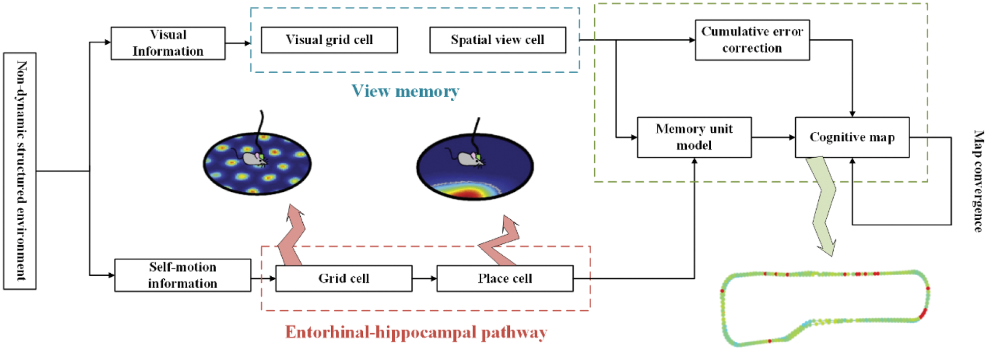
Figure 1: Map construction of the hippocampal cognitive mechanism in the rat-like brain
2.2 Visual Cognitive Memory Calculation Method
In the process of visual cognition, our eyes acquire a stable image from outside and we usually do not notice that our eyeball perform multiple saccades per second. When the eye scans to the next focus, many visual cortex neurons that indicate a specific stimulus predict it before the stimulus reaches the visual receptive field. This process can be described as a series of sensorimotor sequences and predictions after motion positioning. It is not yet clear how the neural network in the brain extracts available information from continuous sensation and movement or how to use the acquired information to predict subsequent sensory stimulation results. Roughly remembering the saccade movement sequence will lead to a huge learning process, because the perceptual movement sequence arrangement can be random for each perceived image.
Therefore, the visual cognitive memory computing model we suggested draws inspiration from how the hippocampus structure predicts the spatial position in the environment. It uses visual grid cells like the grid cell firing pattern to characterize input image information and associates the eyeball focus position with sensory input. It can predict the next position of the eye focus by using the saccade motion signal and then call the sensory features related to that position to predict the sensory input. We set each eye focus sensory input from a small sensory block, including two parallel circuits that use sensory motion sequences to learn and recognize image blocks.
The network structure of this algorithm simulates the mechanism by which visual grid cells provide visual field metrics. We consider that the visual grid cells encode the vectors between the salient stimulus features within the field of view to drive the saccade movement in the period of visual episodic memory. And each time the focus of the eye stays is coded with spatial view cells. The computational framework of the visual cognitive memory model is shown in Fig. 2. In short, the set of visual grid cells uniformly encodes the location points focused in the visual field and any two such locations can be used as input to a vector cell model. The model generates a displacement vector between these two locations from the activity of the visual grid cells and combines this with visual processing. In the learning phase, the gray image collected by the robot body camera is sampled by the square fovea. The feature detector detects the features of the local pixel block encoded by the visual grid cell and establishes the Hebbian connection between the local feature unit and the frame node. Then, learn the relationship between local feature units and the location of these features in the field of view. Finally, all local feature units on this image establishes a two-way connection with the frame node, that is, each frame receives the connection from the local feature unit constituting the feature of the frame and corresponding also has a reverse projection to this local feature unit set.
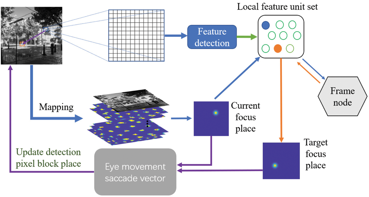
Figure 2: Visual cognitive memory model. The gray image is sampled by the square fovea (blue plaid). The feature detector drives local feature units (blue and orange circles) and each local feature unit encodes a specific salient feature. During learning, each local feature unit is associated with a focal position encoded by a spatial view cell. Local feature unit set is bidirectionally connected to the frame node, which is used to encode the frame being learned. In the recognition stage, when the detected local feature unit triggers the frame node, the local feature unit set selects the focus position of the next local feature unit to be activated (orange feature and orange arrow). The current and target focus positions indicate that the next eye movement saccade vector will be generated
Once the visual memory model has learned the necessary connection relationship, it will test its recognition memory through the next input frame image of the robot. A closed-loop point detection mechanism includes the following processes: 1) The foveal array is centered on a given local feature and the feature detector drives the local feature unit to participate in feature matching; 2) The locally activated feature unit drives its related frame nodes to generate competitive hypotheses about the visual stimulus frame. The most exciting frame node then determines the calculation of the next saccade motion vector from the local feature unit group, which generates a saccade vector. The previously activated local feature unit is reset to zero, and the most exciting frame node uses its return vector to select and detect the next local feature unit to be activated. The gray-scale image is associated with the visual grid cells. The saccade vector of two local features are calculated by the visual grid cells. The spatial view cell coding of the gaze position of the eyeball is activated, which forward input is derived from the coding vector of the visual grid cells. While repeating this step cyclically, the local feature unit will accumulate discharge in the entire recognition cycle until the frame node activation “decision threshold” is reached. That is, the main assumption about the frame node is accepted.
The spatial periodicity of different scales of visual grid cells indicates that they furnish a compact encoding for the two-dimensional space environment and uniquely encode the location information in the space. Similarly, we assume that the visual grid cells also have such characteristics and what is encoded is not a two-dimensional space, but a two-dimensional view plane. For the focal position information in the two-dimensional view plane, we also use spatial view cells with similar place cell characteristics to perform activation discharge expression. The visual grid cell is used as a canonical emissivity map as a table of eyeball focus positions. Each map consists of a matrix of the same size as the focal position table, and is calculated as a 60-degree offset, using Eqs. (1)–(3) to superimpose the cosine wave:
where
For calculating the displacement vector between the two eye focal points, we refer to the oscillating interference model from grid cells to place cells to simulate the activation process from visual grid cells to spatial view cells. Briefly, a given location in the two-dimensional plane is uniquely represented by a set of visual grid cells, a visual grid cell with the appropriate phase in each module is projected to the focal location and activates a spatial view cell. And the relative encoding difference between the two sets of neurons calibrates the sweep vector between the origin and target locations. The connection between activation of the spatial view cell and the eye focal stimulus is generic (independent of the features of the stimulus) and can be established during development. We can consider a two-dimensional vector navigation problem such as this: given the position representation of the sweep starting point
where M denotes the x and y axes, i represents the module scale, and
Among them,
In the learning and memory stage, the location of the gaze point is randomly selected from the input image and coded by visual grid cells and the first gaze focus of each frame will be recorded. Dozens of pixels around the gaze focus are grouped into local pixel blocks. Feature detection is done by a crowd of sensory cells (gaussian adjustment of the preferred gray value) react to the content of each pixel in the part pixel set. The preferred pixel value of the gaussian tuning curve of sensory cell is derived from the blurred image during the memory stage. Depending on the content of the feature detectors, different subsets of these sensory neurons will be in their most active state. That is, for a given feature detector content, the sum of all sensory neurons drives the given local feature label unit to the greatest extent, thus realizing a simple feature detection model. The fuzzy of feature acquisition may result in incorrect initial assumptions about participating stimuli, that is, incorrect frame node are the most active. This assumption will produce saccade positions that will not bring the detector to the expected features. Therefore, sensory cells can drive many local feature units because of accidental partial overlap between their preferred features and what is detected by the fovea. These local feature units transfer certain activities to their related frame nodes.
2.3 Imitation Entorhinal-Hippocampus Self-Motion Information Localization Algorithm
2.3.1 Grid Cell Binary Matrix Acquisition
Place cells are the main dependent neurons for rats to determine their current spatial location and it is also the basis for the establishment of cognitive maps. The grid cell that exist in the entorhinal cortex are also the main input neurons for the place cells in the hippocampus, so there is a need to build a transmission circuit from grid cells to place cells. We propose an iterative model to realize this transfer circuit, which can meet the precise positioning requirements of the robot's position in the current space area. In addition, by adding real-time detection of a single position field in the calculation process of the iterative model, the number of grid field iterations can be dynamically adjusted to increase the precision and efficiency of the algorithm. This algorithm includes the following steps: 1) Get the grid cell firing rate matrix about current area; 2) Binarize the matrix according to the corresponding discharge rate; 3) Iterate successively the binarized matrix obtained from each different grid parameter; 4) Real-time detection of whether there is a single-place field formed. If it has not been generated, it will continue to execute the iteration, otherwise it will stop. The operating process of the iterative model is shown in Fig. 3.
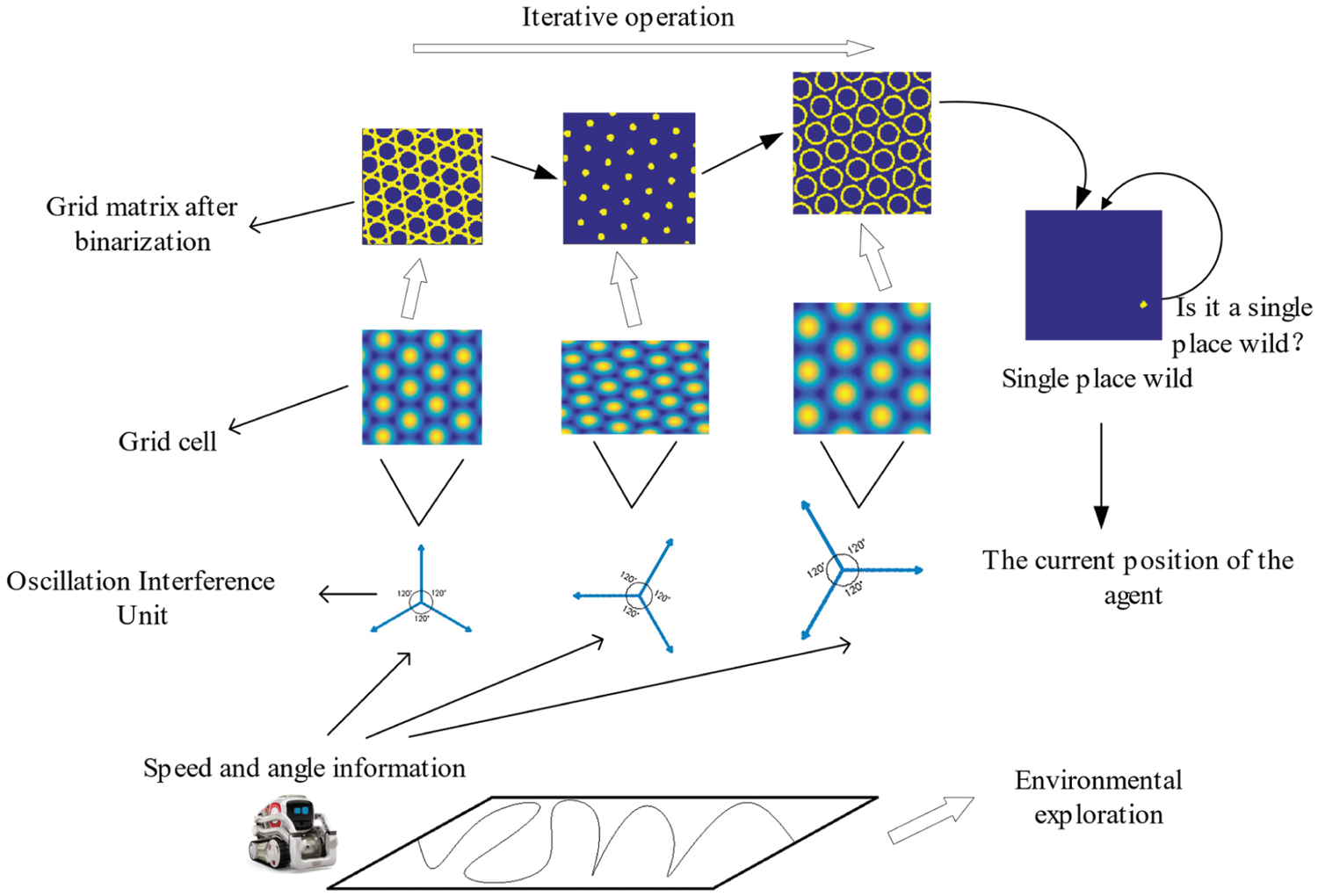
Figure 3: Obtaining robot body position information through iterative models
First, the mathematical expression of the discharge rate
Among them,
where
Suppose the area is a rectangular area with length and width respectively L and D. The grid field of the grid cells in the rectangular area is essentially a matrix
In the Eq. (9), T represents the current grid cell discharge rate;
2.3.2 Iterative Solution of Place Cell Discharge Field
Suppose there are i grid fields, after the discharge rate matrix and binarization solution, i binary matrix
After each iteration of the calculation, the binary matrix will transfer its location information to the place matrix. With the increase of the number of iterations, the possible locations of the agent on the position matrix gradually decrease, which indicates the position of the agent is gradually clear. Numerous calculation experiments have found that simply using the iterative model to solve the position field may result in multiple position fields on the obtained position matrix. This situation may be caused by insufficient number of iterations, or it may be that a single position field has been generated on the position matrix when the number of iterations is less than the set number. Therefore, the number of iterative calculations must be reasonable. The solution algorithm with a fixed number of iterations cannot guarantee the accuracy and efficiency of the algorithm, a method of changing the number of iterations is required. A real-time detection process for the position matrix is added. After each iteration calculation is completed, it is judged whether a single position field has been generated on the position matrix, and this is the basis for judging whether it is necessary to increase the number of iterations. The schematic diagram of the iterative solution process of place field detection is shown in Fig. 4.
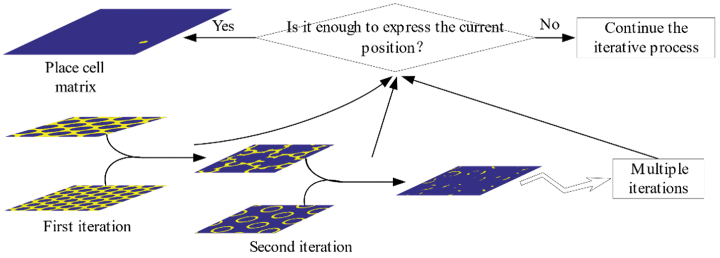
Figure 4: Place field detection iterative solving process
Search for the element of
2.4 Cognitive Map Construction Method
Cognitive map is an internal expression of the external space environment. We refer to the construction method of experience map in RatSLAM algorithm [37] to construct cognitive map, as shown in Fig. 5 for a schematic diagram of cognitive map construction.
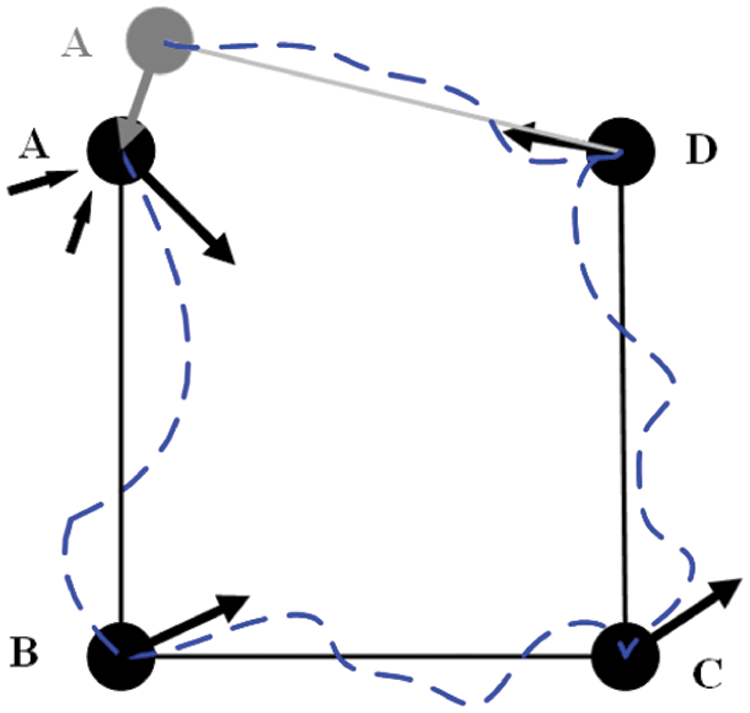
Figure 5: Cognitive map diagram
This cognitive map is a topological structure, which contains information about the firing field activity of the place cell and the environmental information of visual memory. The cognitive map is composed of many cognitive nodes e with topological relationships, and the cognitive nodes are represented by the relationship
In the Eq. (11),
As the robot continues to move in the environment, the scale of the environment map will continue to increase. However, since the iterative model from grid cells to place cells is only limited to cognition in a given spatial area, we introduce the concept of local location recognition reset for this purpose. The specific strategy is that when the robot reaches the boundary of the predetermined coding area, the grid cell phase will be periodically reset, so that the mobile robot is again at the center of the rectangular area covered by the grid field after the reset. Through this method, each time the grid cell phase is reset, the place cell can immediately generate a position code for a new spatial region to realize the position recognition of the rat in any size spatial region. The local location recognition reset process is shown in Fig. 6.
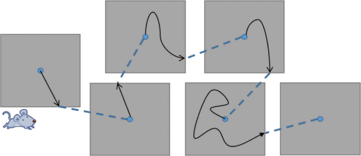
Figure 6: Mechanisms of position perception under periodic resetting of grid cell phase
With the continuous exploration of the robot in the environment, the location-specific discharge activity of the cells will fill the entire environmental space that it walks over time. At the same time, the cognitive nodes of the cognitive map will continue to increase with the discharge of the place cells. Setting an initial position recognition to the node
Among them,
An evaluation parameter S is used to compare the matching degree between the activity information of the cell at the current position and the corresponding position information in the existing cognitive node as Eq. (13).
When S does not reach the set threshold, detect the local feature unit and its corresponding vector relationship in the visual image memory. If the visual memory reaches the recognition threshold condition, it means that the current position information and environmental characteristics of the robot have passed by here during the previous movement. That is, it is considered that it has returned to the place that the robot has experienced before, which is the so-called closed loop point. When S exceeds the set threshold, only a new cognitive map node is created, and the visual inspection process is not performed.
As the cognitive node e continues to accumulate, its relative error is also accumulating. When the closed loop point is reached, the position integrated by the path on the cognitive map will be mismatched with the current actual position. The relative relaxation of the topological structure of the experience map is to minimize the error between the change of the integral error and the absolute position and use its topological structure to adjust the position of the cognitive node as shown in Eq. (14). The correction mechanism of cognitive map is continuous, and the error correction is more obvious at the closed loop point.
Among them,
With the accumulation of time in construction, the above algorithm will inevitably cause the redundancy of experience points resulting in a cognitive map with too many redundant nodes, which is difficult to maintain and manage a map sequence. Therefore, the sequence of cognitive nodes must be maintained at a level that can be managed and preserved. The pruning of the cognitive map is achieved by setting the maximum node density threshold in the space, so that the finally formed cognitive map has nothing to do with the exploration time of the robot and is proportional to the size of the exploration space. Its realization method is as shown in Eq. (15).
Among them, e is a collection of cognitive nodes and g is a collection of cognitive map grid blocks. As shown in Fig. 7, when the cognitive node A already exists in a grid block and the new cognitive node B also appears in the grid, the cognitive node B is deleted, the nodes related to B are linked to A.
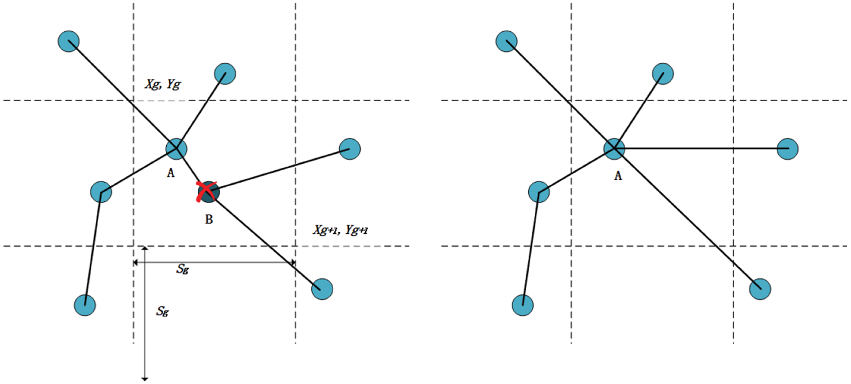
Figure 7: Deletion of cognitive nodes. Before trimming (left), after trimming (right)
3.1 Simulation Experiment Results of the Iterative Algorithm
The cognitive map constructed in this article is a dynamic incremental location cognitive map model based on the activation of the firing process of place cells at a specific location and the integration of visual memory units. Therefore, the accuracy of the iterative model algorithm designed in the previous article. It is essential to establish a complete spatial cognitive map. In the experiment, the rectangular area of cell activation at a given single location was set to a space size of 40 cm × 40 cm and 8 grid cell modules were used to generate the corresponding grid cell binary matrix. The characteristic parameters of the grid field corresponding to the 8 grid cell modules are: grid field orientation
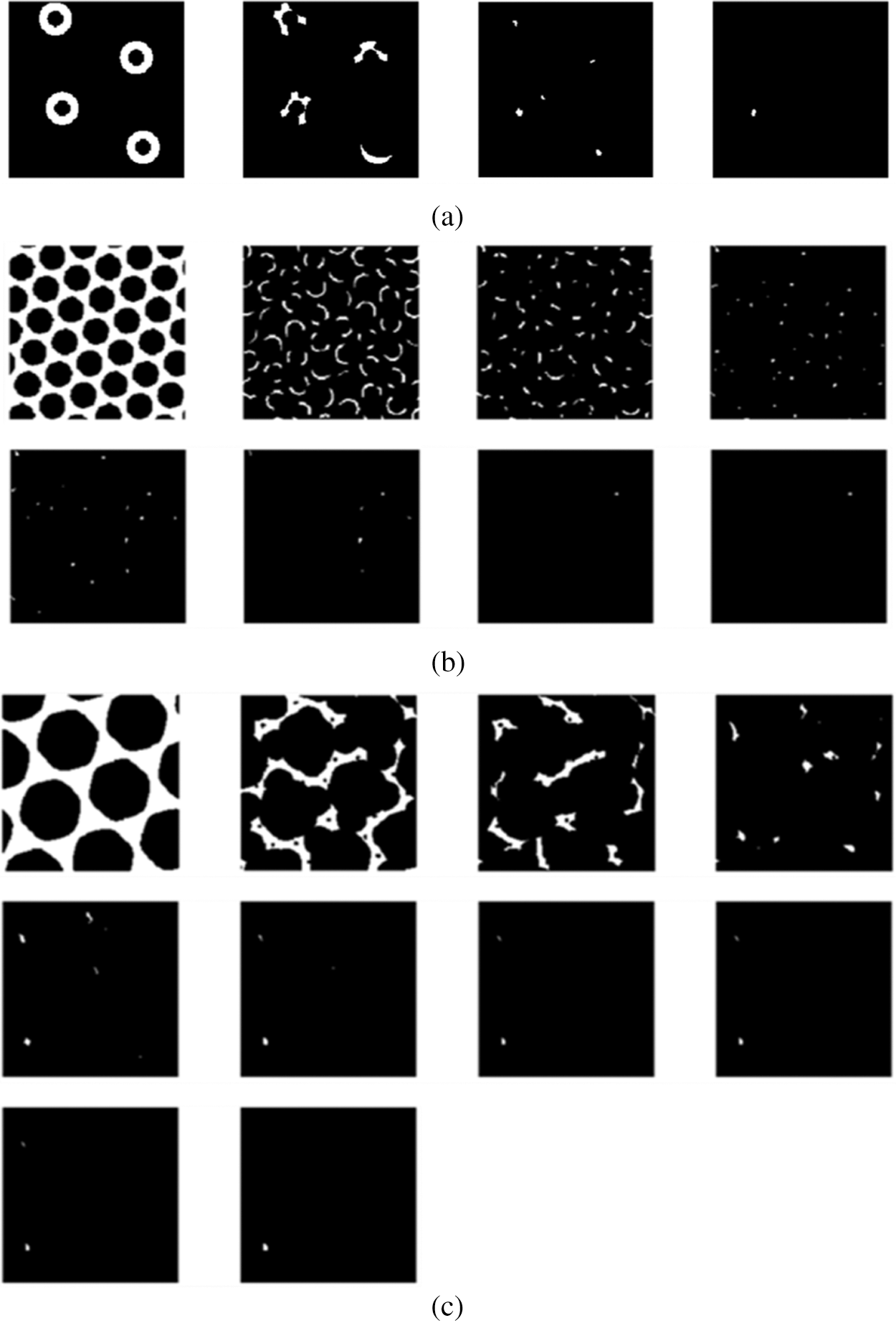
Figure 8: Schematic diagram of single-place field activation discharge calculated by iterative algorithm. Comparing the results of the three times, too many or too few iterative calculations cannot guarantee the accuracy of position expression. (a) After 4 iterations of calculation, the process of forming a place cell discharge field at a single location. (b) After 7 iterations of calculation, the process of forming a single place cell discharge field. (c) After 10 iterations of calculation, the process of forming a single place cell discharge field
3.2 Visual Cognitive Memory Experiment
When the robot starts to move from the initial position, the image frames recorded by the camera will be learned at regular intervals. Frame nodes, local feature unit set, and visual grid cells will be associated. Next, the images collected by the mobile robot will be compared with the recorded image frames. The recognition memory driven by the visual grid cells will take over this process and calculate the saccade vectors for the predicted positions of other stimulus features. Detecting the first perceptual local feature unit also means generating a hypothesis of the scene experienced in the past, and the main hypothesis (this mean the most active frame node neuron) determines the continuous saccade to confirm the hypothesis. Fig. 9 shows the image frame recognition process of this model when running the Bicocca data set [38]. Each eye vector saccade means moving a different local feature part to the focus of the eye. Once the feature detection reaches the recognition threshold, it will continue to scan to the next local feature. We set a recognition (decision) threshold of 0.9, and each sweep represents a move of the local feature stimulus to the eye focus. When the cumulative local feature recognition reaches the recognition threshold, it means that this frame has been learned and remembered before, and this frame is also the closed-loop point for the mobile robot to build a map, at which point the cumulative error with the previous closed-loop point on the map is corrected.
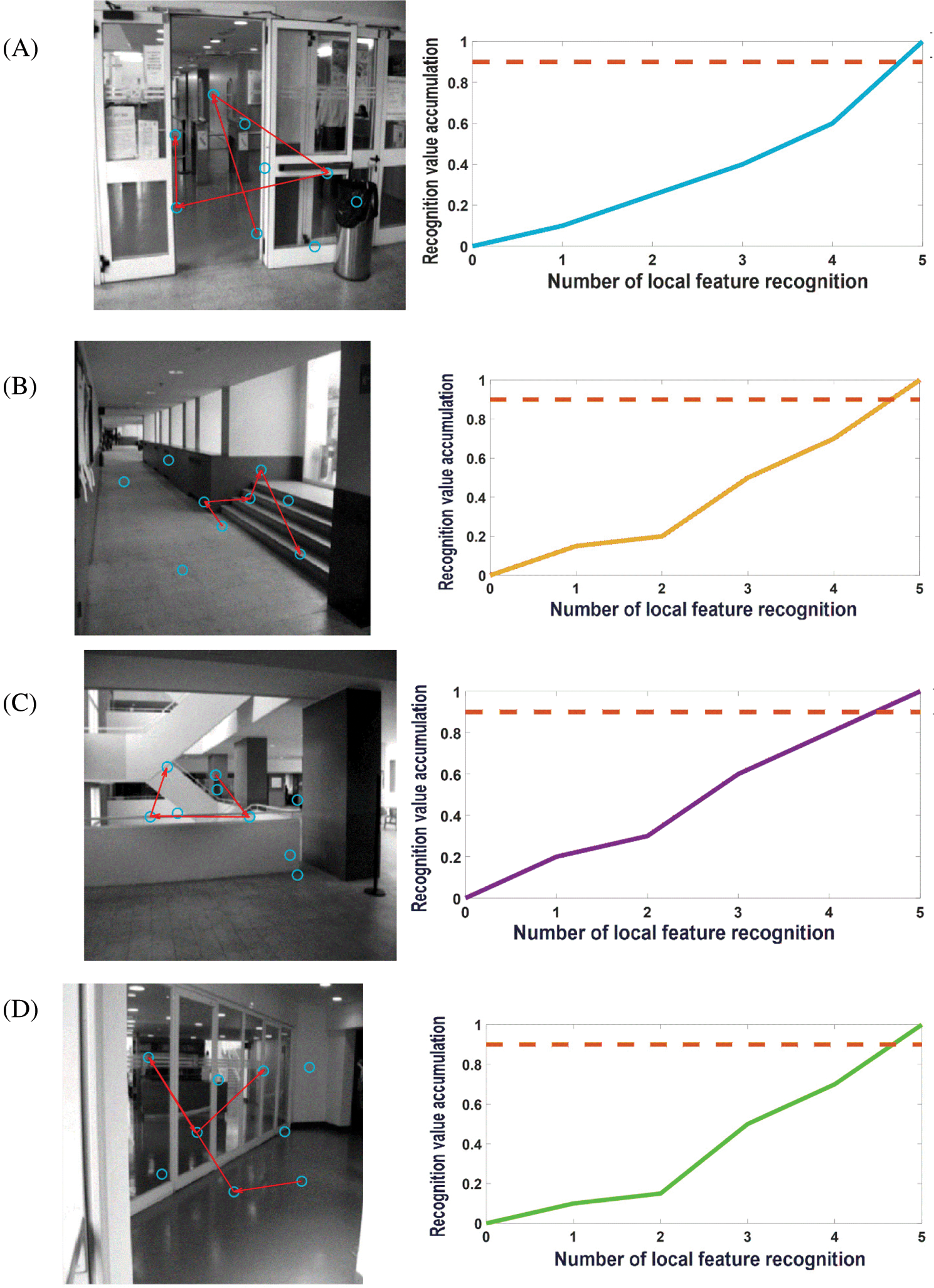
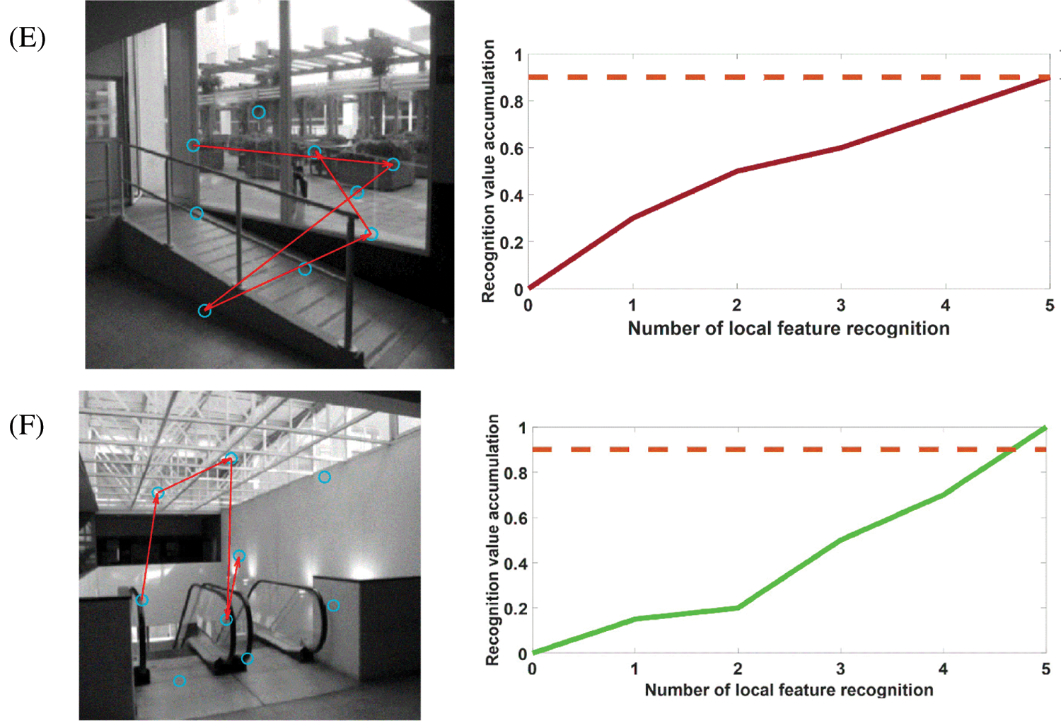
Figure 9: Pictures A–F are examples of recognition of some image frames when running the Bicocca data set [38]. Most images can be recognized in the process of four saccades. The blue circle represents the center of the image's local features; the red line represents the saccade movement of the eyeball; the dotted line represents the decision threshold. For each local feature, after the recognition is successful, the recognition activation rate of the image frame will increase until it reaches the recognition threshold
3.3 Cognitive Map Construction
To verify the validity of the cognitive map construction method proposed, we designed three experiments: 1) Simulation experiments based on the public data set Bicocca; 2) Use the robot platform equipped with this model to explore the scene in the laboratory and record the data to build a cognitive map; 3) Compare the model in this article with the classic rat-like brain mapping algorithm RatSLAM.
The public data set Bicocca (indoor) was collected by a mobile robot in a building of the University of Bicocca in Milan. The data set contains 68083 images. The part of the location explored by the robot during the collection of the data set consists of the ground floor of the office building and the corresponding floor of the adjacent building. The two buildings are connected by a glass-walled bridge with a roof. A plan view of the dataset building is shown in Fig. 10a, while Fig. 10b shows the path trajectory of part of the dataset used in the experiment.
Figure 10: (a) Building plan of the Bicocca data set. (b) Path trajectory diagram of part of the data set used in the algorithm of this article (red line)
Before the model runs, it is necessary to pre-train the grid cells to pre-encode the position of each pixel in the input image area to calculate the eye focus and eye saccade vector during the run. Before the model runs, it is necessary to pretrain the grid cells to pre-encode the position of each pixel in the input image area to calculate the eye focus and eye saccade vector during the run. In addition, in the model calculation process, all RGB images in the input data set will be uniformly converted into grayscale images to reduce the amount of calculation and one frame per 100 frames is selected as a visual memory point. Fig. 11 shows the running results of the constructed cognitive map at different times. It can be seen from Figs. 11a–11d that as the robot moves, the cumulative error of sensors such as the odometer becomes larger and larger. Cause the trajectory of the robot deviates from the original trajectory, which has a large deviation from the actual path and the trajectory is relatively messy. However, the cognitive map can successfully detect the closed loop, correct the path and successfully construct the environmental map.
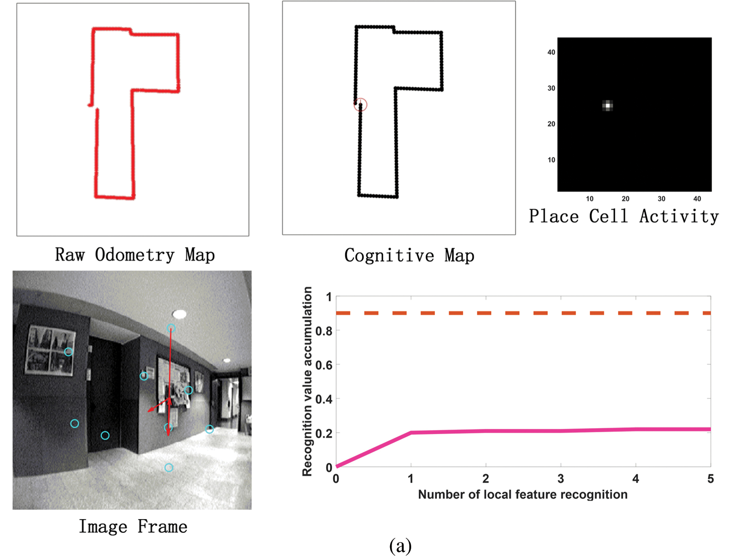
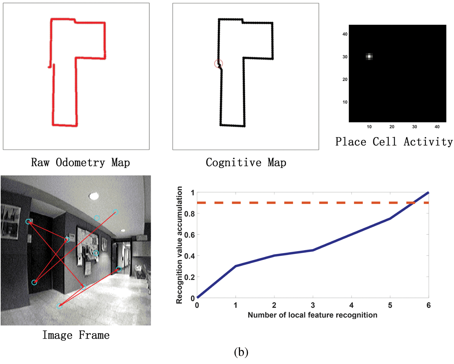
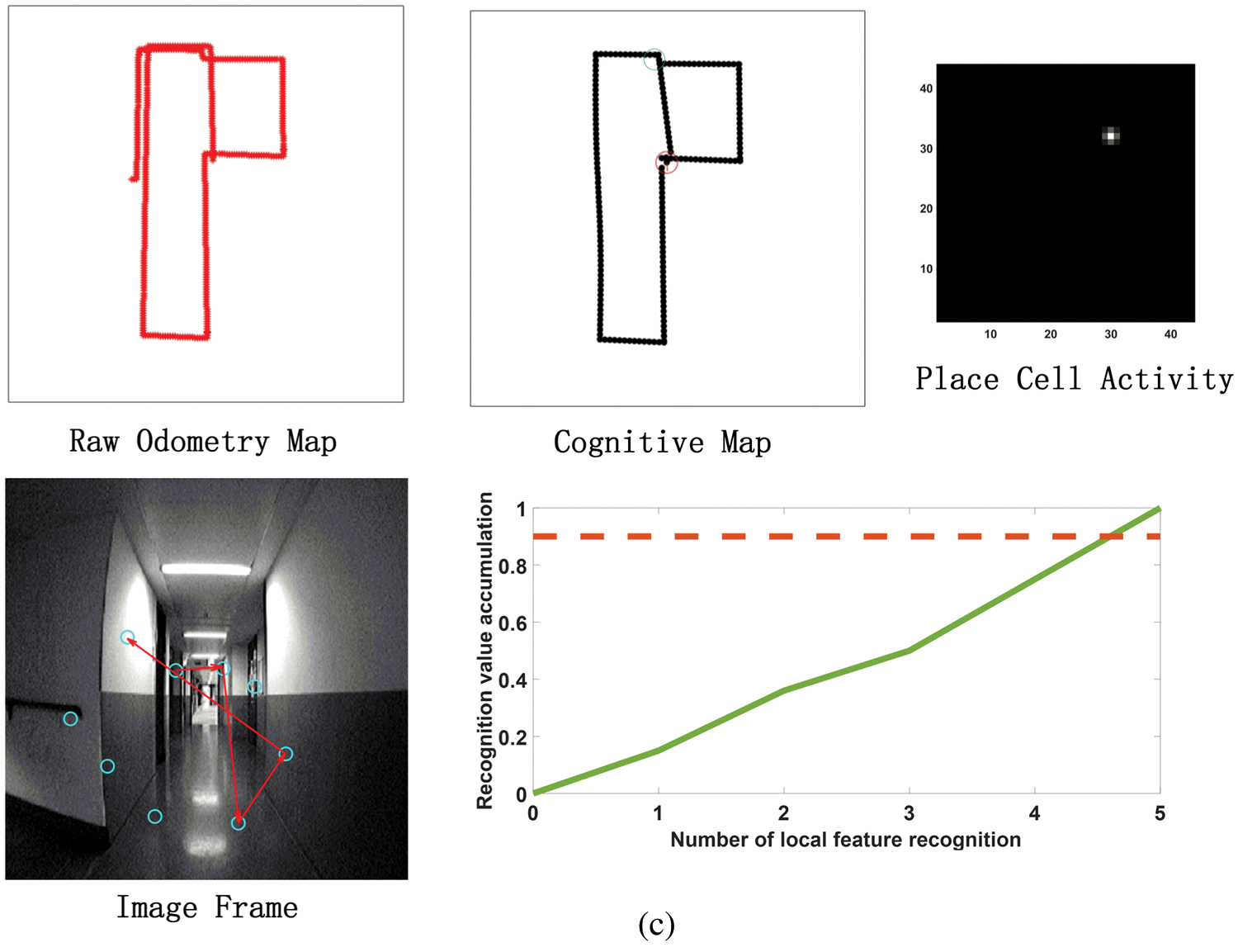
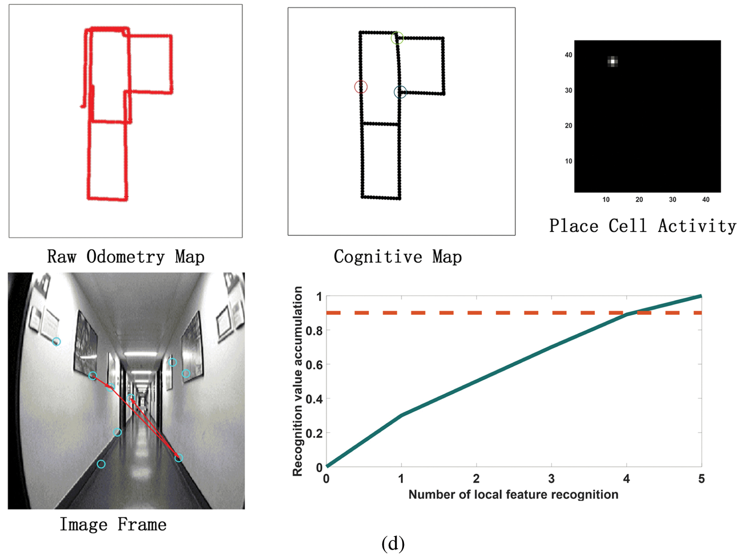
Figure 11: The process of building a cognitive map. (a) The mapping situation of the algorithm model when it is close to the closed-loop point but does not reach the closed-loop point when the algorithm model has nearly completed a week. Before reaching the closed loop point, the original odometer and the constructed cognitive map are almost the same. Since the closed-loop point of the map has not been reached, the first local feature of the image frame detected an incorrect assumption, and the subsequent appropriate amount of motion failed to be detected, so the closed-loop point was not reached. (b) The mapping situation of the algorithm model at the closed loop point after the completion of a week. At the closed-loop point, the original odometer has a deviation and fails to close with the position at the closed-loop point. The visual memory model recognizes the closed loop points, and the cognitive map achieves closure. (c) After the algorithm model passes through the closed-loop point (the green circle on the cognitive map) for the second time, the map is shifted due to the influence of the error caused by the original odometer. (d) After passing through two closed-loop points (the green and blue circles in the cognitive map), the method of setting the maximum node density threshold described in this article is used to correct the map offset in Fig. 11c
The Turtlebot2 robotic platform was used to provide the physical basis for this experiment. It has a mobile robot base, a red-green-blue-depth (RGB-D) camera, two motor encoders (providing odometer information) and a micro-inertial measurement unit (MIMU, providing angular information). When the robot is building a cognitive map, it needs to receive the motion instructions sent by the computer. Therefore, it is necessary to place the laptop on the robot platform and control the robot to move in the environment through the wireless keyboard, and receive the speed, direction and image information. We control the mobile robot to explore in a 3 m × 10 m laboratory environment, the exploration time is 240 s, the sampling period is 0.2 s, and the maximum moving speed of the mobile robot platform during the collection process is set to 0.5 m/s. Fig. 12a the actual robot motion trajectory (shown by the blue line) and Fig. 12b are the robot platform used in the experiment and the images collected in some laboratories.
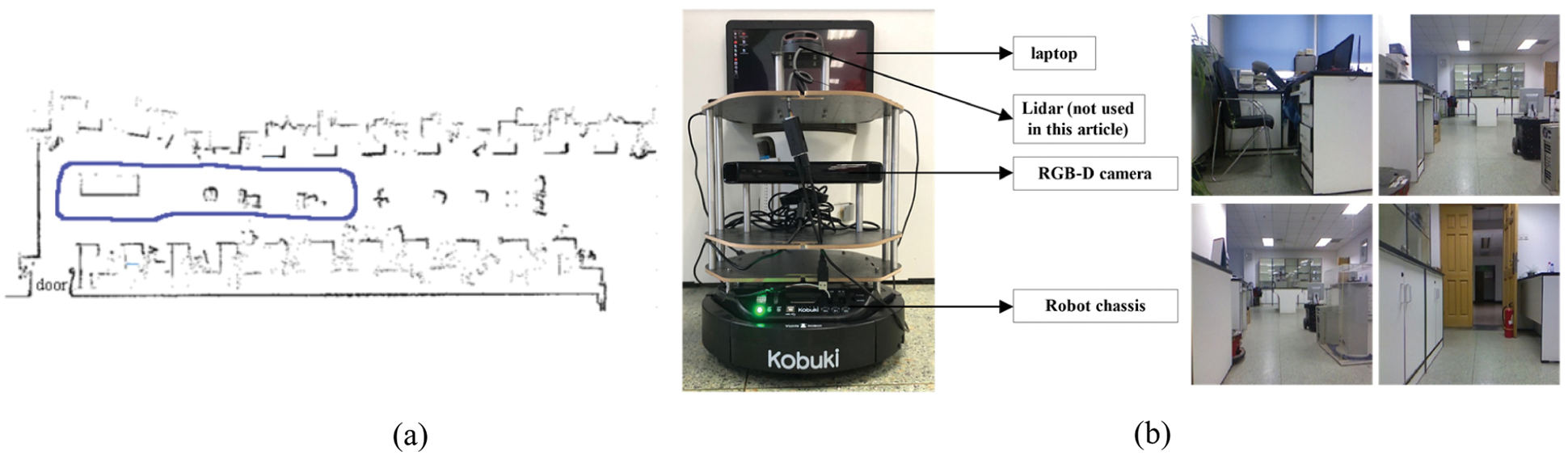
Figure 12: (a) The actual trajectory of the robot. (b) Mobile robot platform and some laboratory images collected
We use the algorithm in this article to build a cognitive map of an indoor laboratory and the RatSLAM algorithm builds a map under this data set for comparison experiments. The closed-loop detection method adopted by the RatSLAM algorithm is to use the scanline intensity profile in the depth image to match the view template and then complete the correction of the cumulative error of the cognitive map. Fig. 13 shows the comparison of the original odometer movement route (left), the RatSLAM algorithm (middle) and the cognitive map established by the algorithm of this article (right). From the experimental results, the cognitive map established by the algorithm in this paper is basically the same as the odometer map. However, as the robot moves, the cumulative error of sensors such as the odometer becomes larger and larger, which causes the robot trajectory to deviate from the original trajectory, which has a large deviation from the actual path, and the trajectory is relatively messy. However, the cognitive map can successfully detect the closed loop, correct the path and draw an accurate cognitive map. From the comparison chart in Figs. 13c and 13d, both the algorithm in this article and the RatSLAM algorithm can detect closed loop points and correct the path. However, with the increase of operation time, the cognitive map established by RatSLAM has drifted, but the algorithm in this article still maintains good robustness.
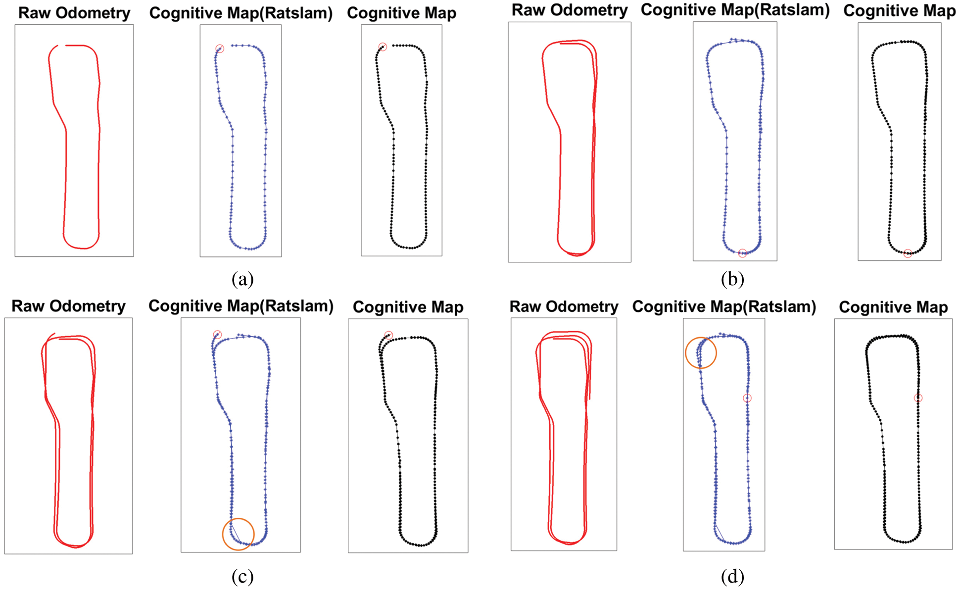
Figure 13: At different time nodes, the original odometer (left), RatSLAM algorithm (middle) are compared with our algorithm. (a) Comparison of experimental results at 80 s. The cognitive map and odometer map established by the two algorithms are basically the same, but the cognitive map established by our algorithm is denser. Compared with the pose cells proposed by RatSLAM, the iterative algorithm in this paper can generate more accurate position recognition nodes. (b) Comparing the experimental results at 140 s, the trajectory recorded by the odometer began to drift. After running around the map for a week, the RatSLAM algorithm failed to achieve the closed loop of the map. The algorithm we proposed successfully achieved the closed loop of the map. (c) Comparison of experimental results at 180 s. The cognitive map established by RatSLAM's algorithm shows large positional shifts (orange circles), but the algorithm in this article is still accurate. (d) Compared with the experimental results at 240 s, the RatSLAM algorithm failed to correct the cumulative error after detecting the closed loop point, and realized the map closure, while our algorithm established a complete cognitive map
Our algorithm uses the relative positions of visual image features to identify closed-loop points to correct the established cognitive map. We discuss how spatially separated sensory inputs (encoding eye focus positions with visual grid cells) can collaborate in parallel to identify closed-loop points, and this is the first approach to identify map closed-loop points using spatially separated sensory inputs. The core theoretical basis of this approach is that visual recognition memory will use visual grid cells to encode the relative layout of multiple features. The model has been simplified accordingly to focus on the basic mechanisms proposed, such as pre-processing of the input image with conventional feature detection methods.
It is inevitable that physical factors such as wheel slip will cause cumulative errors during robot movement, but our algorithm does a good job of correcting for map errors, demonstrating the better environmental adaptability and robustness. Although the RatSLAM algorithm is a classic rat brain hippocampus mapping scheme, the pose cell it uses is a virtual cell type that assists in mapping and navigation and is not a real biological brain cell. However, the various cell types used in our mapping algorithm (especially grid cells and place cells, which are key cell types for mammalian positioning and navigation) are present in the mammalian brain. In addition, the visual memory model proposed by our algorithm characterizes the perceptual mechanism of biological vision, establishes the encoding of the position of the eye during image recognition and the encoding of information at the eye focus, and corresponds one-to-one to the recognition cognitive mechanism of mammals found in biological experiments, so our algorithm is more suitable for the study of robotic bionics.
We propose a bionic cognitive map construction system incorporating bio-vision, which features an iterative model computational approach to establish a grid cell to location cell discharge activation process for robot localization in space. Furthermore, inspired by the results of experiments in mammalian physiology, this model employs an image memory algorithm based on visual grid cells and spatial view cells to close the loop on the established cognitive maps and correct for errors in spatial cell path integration. Grid cells and place cells underlie spatial localization and navigation in rats, however, similar firing activity in the visual paradigm suggests that the same neural circuits may also contribute to visual processing. Sensory signals from rat vestibular and proprioceptive movements can drive grid cells and position cells during path integration and large-scale spatial navigation, and when an intelligent body is engaged in a visual recognition task, oculomotor sweep neural inputs can update similar cells for scene memory. This visual memory approach shows how one-shot learning occurs in the robot's environment, like one-shot learning in the hippocampal structure of the rat brain. The model ultimately constructs a topological metric map containing the coordinates of environmental location points, visual scene cues and bit-specific topological relationships. Unlike the traditional closed-loop detection approach in SLAM algorithms, our closed-loop detection algorithm plays a specific role of visual grid cells in visual recognition, which is consistent with recent evidence on visual grid cells driven by eye movements [39–41]. Comparing the rat-like brain map building algorithm RatSLAM, our algorithm performs better in terms of environmental adaptation and robustness, and the whole algorithmic framework is more in line with facts from biophysiological studies rather than using virtual pose cells. Our proposed cognitive map construction method is based on biological environmental cognitive mechanisms and visual situational memory mechanisms and will provide a basis for further research on bionic robot navigation.
Acknowledgement: Thanks to the Key Laboratory of Computational Intelligence and Intelligent Systems, Beijing University of Technology for their help in the experiments in this article.
Funding Statement: This research was funded by the National Science Foundation of China, Grant No. 62076014, as well as the Beijing Natural Science Foundation under Grant No. 4162012.
Conflicts of Interest: The authors declare that they have no conflicts of interest to report regarding the present study.
1. Dissanayake, M. W. M. G., Newman, P., Clark, S., Durrant-Whyte, H. F., Csorba, M. (2013). A solution to the simultaneous localization and map building (SLAM) problem. IEEE Transactions on Robotics and Automation, 17(3), 229–241. DOI 10.1109/70.938381. [Google Scholar] [CrossRef]
2. Barbara, L., Ray, J. (1993). “What” and “where” in spatial language and spatial cognition. Behavioral & Brain Sciences, 16(2), 217–238. DOI 10.1017/S0140525X00029733. [Google Scholar] [CrossRef]
3. Burgess, N., Maguire, E. A., O'Keefe, J. (2002). The human hippocampus and spatial and episodic memory. Neuron, 35(4), 625–641. DOI 10.1016/S0896-6273(02)00830-9. [Google Scholar] [CrossRef]
4. Robin, J. (2018). Spatial scaffold effects in event memory and imagination. Wiley Interdisciplinary Reviews Cognitive Science, 9(4), e1462. DOI 10.1002/wcs.1462. [Google Scholar] [CrossRef]
5. Bonnevie, T., Dunn, B., Fyhn, M., Hafting, T., Derdikman, D. et al. (2013). Grid cells require excitatory drive from the hippocampus. Nature Neuroscience, 16(3), 309–317. DOI 10.1038/nn.3311. [Google Scholar] [CrossRef]
6. Moser, E. I., Kropff, E., Moser, M. B. (2008). Place cells, grid cells, and the brain's spatial representation system. Annual Review of Neuroscience, 31(1), 69–89. DOI 10.1146/annurev.neuro.31.061307.090723. [Google Scholar] [CrossRef]
7. Harvey, C. D., Collman, F., Dombeck, D. A., Tank, D. W. (2009). Intracellular dynamics of hippocampal place cells during virtual navigation. Nature, 461(7266), 941–946. DOI 10.1038/nature08499. [Google Scholar] [CrossRef]
8. Foster, D., Wilson, M. (2006). Reverse replay of behavioural sequences in hippocampal place cells during the awake state. Nature, 440(7084), 680–683. DOI 10.1038/nature04587. [Google Scholar] [CrossRef]
9. Jauffret, A., Cuperlier, N., Gaussier, P. (2015). From grid cells and visual place cells to multimodal place cell: A new robotic architecture. Frontiers in Neurorobotics, 9, 1. DOI 10.3389/fnbot.2015.00001. [Google Scholar] [CrossRef]
10. Yu, N., Wang, L., Jiang, X., Yuan, Y. (2020). An improved bioinspired cognitive map-building system based on episodic memory recognition. International Journal of Advanced Robotic Systems, 17(3), 172988142093094. DOI 10.1177/1729881420930948. [Google Scholar] [CrossRef]
11. Savelli, F., Luck, J. D., Knierim, J. J. (2017). Framing of grid cells within and beyond navigation boundaries. Elife, 6, e21354. DOI 10.7554/eLife.21354. [Google Scholar] [CrossRef]
12. Krupic, J., Bauza, M., Burton, S., O'Keefe, J. (2018). Local transformations of the hippocampal cognitive map. Science, 359(6380), 1143. DOI 10.1126/science.aao4960. [Google Scholar] [CrossRef]
13. Yan, C., Wang, R., Qu, J., Chen, G. (2016). Locating and navigation mechanism based on place-cell and grid-cell models. Cognitive Neurodynamics, 10(4), 1–8. DOI 10.1007/s11571-016-9384-2. [Google Scholar] [CrossRef]
14. Huhn, Z., Somogyvári, Z., Kiss, T., Erdi, P. (2009). Distance coding strategies based on the entorhinal grid cell system. Neural Networks, 22(5–6), 536–543. DOI 10.1016/j.neunet.2009.06.029. [Google Scholar] [CrossRef]
15. Nau, M., Navarro Schröder, T., Bellmund, J. L. S., Doeller, C. F. (2018). Hexadirectional coding of visual space in human entorhinal cortex. Nature Neuroscience, 21(2), 188–190. DOI 10.1038/s41593-017-0050-8. [Google Scholar] [CrossRef]
16. Lucas, H. D., Duff, M. C., Cohen, N. J. (2019). The Hippocampus promotes effective saccadic information gathering in humans. Journal of Cognitive Neuroscience, 31(2), 186–201. DOI 10.1162/jocn_a_01336. [Google Scholar] [CrossRef]
17. Hoffman, K. L., Dragan, M. C., Leonard, T. K., Micheli, C., Montefusco-Siegmund, R. et al. (2013). Saccades during visual exploration align hippocampal 3–8 Hz rhythms in human and non-human primates. Frontiers in Systems Neuroscience, 7, 43. DOI 10.3389/fnsys.2013.00043. [Google Scholar] [CrossRef]
18. Fraedrich, E. M., Flanagin, V. L., Duann, J. R., Brandt, T., Glasauer, S. (2012). Hippocampal involvement in processing of indistinct visual motion stimuli. Journal of Cognitive Neuroscience, 24(6), 1344–1357. DOI 10.1162/jocn_a_00226. [Google Scholar] [CrossRef]
19. Matthias, N., Julian, J. B., Doeller, C. F. (2018). How the brain's navigation system shapes our visual experience. Trends in Cognitive Sciences, 22(9), 810–825. DOI 10.1016/j.tics.2018.06.008. [Google Scholar] [CrossRef]
20. Robertson, R. G., Rolls, E. T., Ois, G. F. (1998). Spatial view cells in the primate hippocampus: Effects of removal of view details. Journal of Neurophysiology, 79(3), 1145–1156. DOI 10.1152/jn.1998.79.3.1145. [Google Scholar] [CrossRef]
21. Rolls, E. T. (1999). Spatial view cells and the representation of place in the primate hippocampus. Hippocampus, 9(4), 467–480. DOI 10.1002/(ISSN)1098-1063. [Google Scholar] [CrossRef]
22. Duhamel, C. L., Goldberg, M. E. (1992). The updating of the representation of visual space in parietal cortex by intended eye movements. Science, 255(5040), 90–92. DOI 10.1126/science.1553535. [Google Scholar] [CrossRef]
23. Stigchel, S., Meeter, M., Theeuwes, J. (2006). Eye movement trajectories and what they tell us. Neuroscience & Biobehavioral Reviews, 30(5), 666–679. DOI 10.1016/j.neubiorev.2005.12.001. [Google Scholar] [CrossRef]
24. Jeff, H., Subutai, A., Cui, Y. (2017). A theory of How columns in the neocortex enable learning the structure of the world. Frontiers in Neural Circuits, 11, 81. DOI 10.3389/fncir.2017.00081. [Google Scholar] [CrossRef]
25. Keech, T. D., Resca, L. (2010). Eye movement trajectories in active visual search: Contributions of attention, memory, and scene boundaries to pattern formation. Attention Perception & Psychophysics, 72(1), 114–141. DOI 10.3758/APP.72.1.114. [Google Scholar] [CrossRef]
26. Nicosevici, T., Garcia, R. (2012). Automatic visual Bag-of-words for online robot navigation and mapping. IEEE Transactions on Robotics, 28(4), 886–898. DOI 10.1109/TRO.2012.2192013. [Google Scholar] [CrossRef]
27. Mitash, C., Bekris, K. E., Boularias, A. (2017). A self-supervised learning system for object detection using physics simulation and multi-view pose estimation. IEEE/RSJ International Conference on Intelligent Robots and Systems, pp. 545–551. Vancouver, BC, Canada. [Google Scholar]
28. Wu, H., Wu, Y. X., Liu, C. A., Yang, G. T., Qin, S. Y. et al. (2016). Fast robot localization approach based on manifold regularization with sparse area features. Cognitive Computation, 8(5), 1–21. DOI 10.1007/s12559-016-9427-3. [Google Scholar] [CrossRef]
29. Li, R., Wang, S., Gu, D. (2020). DeepSLAM: A robust monocular SLAM system with unsupervised deep learning. IEEE Transactions on Industrial Electronics, 68(4), 3577–3587. DOI 10.1109/TIE.2020.2982096. [Google Scholar] [CrossRef]
30. Werner, F., Sitte, J., Maire, F. (2012). Topological map induction using neighbourhood information of places. Autonomous Robots, 32(4), 405–418. DOI 10.1007/s10514-012-9276-1. [Google Scholar] [CrossRef]
31. Yarbus, A. L. (1967). Eye movements during perception of complex objects. In: Eye movements & vision, pp. 171–211. Boston, MA: Springer. [Google Scholar]
32. Rayner, K. (1978). Eye movements in reading and information processing: 20 years of research. Psychological Bulletin, 85(3), 618–660. DOI 10.1037/0033-2909.85.3.618. [Google Scholar] [CrossRef]
33. Martinez-Conde, S., Macknik, S. L., Hubel, D. H. (2004). The role of fixational eye movements in visual perception. Nature Reiview Neuroscience, 5(3), 229–240. DOI 10.1038/nrn1348. [Google Scholar] [CrossRef]
34. Hawkins, J., Lewis, M., Klukas, M., Purdy, S., Ahmad, S. (2019). A framework for intelligence and cortical function based on grid cells in the neocortex. Frontiers in Neural Circuits, 12, 121. DOI 10.3389/fncir.2018.00121. [Google Scholar] [CrossRef]
35. Bicanski, A., Burgess, N. (2019). A computational model of visual recognition memory via grid cells. Current Biology, 29(6), 979–990.e4. DOI 10.1016/j.cub.2019.01.077. [Google Scholar] [CrossRef]
36. Laptev, D., Burgess, N. (2019). Neural dynamics indicate parallel integration of environmental and self-motion information by place and grid cells. Frontiers in Neural Circuits, 13, 59. DOI 10.3389/fncir.2019.00059. [Google Scholar] [CrossRef]
37. Ball, D., Heath, S., Wiles, J., Wyeth, G., Corke, P. et al. (2013). OpenRatSLAM: An open source brain-based SLAM system. Autonomous Robots, 34(3), 149–176. DOI 10.1007/s10514-012-9317-9. [Google Scholar] [CrossRef]
38. Civera, J., Grasa, O. G., Davison, A. J., Montiel, J. M. M. (2009). 1-Point RANSAC for EKF-based structure from motion. IEEE/RSJ International Conference on Intelligent Robots & Systems, pp. 3498–3504. St. Louis, MO, USA. [Google Scholar]
39. Killian, N. J., Jutras, M. J., Buffalo, E. A. (2012). A map of visual space in the primate entorhinal cortex. Nature, 491(7426), 761–764. DOI 10.1038/nature11587. [Google Scholar] [CrossRef]
40. Killian, N. J., Potter, S. M., Buffalo, E. A. (2016). Saccade direction encoding in the primate entorhinal cortex during visual exploration. Proceedings of the National Academy of Sciences of the United States of America, 112(51), 15743–15748. DOI 10.1073/pnas.1417059112. [Google Scholar] [CrossRef]
41. Jutras, M. J., Fries, P., Buffalo, E. A. (2013). Oscillatory activity in the monkey hippocampus during visual exploration and memory formation. Proceedings of the National Academy of Sciences of the United States of America, 110(32), 13144–13149. DOI 10.1073/pnas.1302351110. [Google Scholar] [CrossRef]
 | This work is licensed under a Creative Commons Attribution 4.0 International License, which permits unrestricted use, distribution, and reproduction in any medium, provided the original work is properly cited. |