| Computer Modeling in Engineering & Sciences |
DOI: 10.32604/cmes.2022.018596
ARTICLE
Isogeometric Analysis with Local Adaptivity for Vibration of Kirchhoff Plate
College of Civil Engineering and Architecture, Key Laboratory of Disaster Prevention and Structural Safety of Ministry of Education, Guangxi Key Laboratory of Disaster Prevention and Structural Safety, Guangxi University, Nanning, 530000, China
*Corresponding Author: Sheng He. Email: hesheng@gxu.edu.cn
Received: 10 August 2021; Accepted: 30 August 2021
Abstract: Based on our proposed adaptivity strategy for the vibration of Reissner–Mindlin plate, we develop it to apply for the vibration of Kirchhoff plate. The adaptive algorithm is based on the Geometry-Independent Field approximaTion (GIFT), generalized from Iso-Geometric Analysis (IGA), and it can characterize the geometry of the structure with NURBS (Non-Uniform Rational B-Splines), and independently apply PHT-splines (Polynomial splines over Hierarchical T-meshes) to achieve local refinement in the solution field. The MAC (Modal Assurance Criterion) is improved to locate unique, as well as multiple, modal correspondence between different meshes, in order to deal with error estimation. Local adaptivity is carried out by sweeping modes from low to high frequency. Numerical examples show that a proper choice of the spline space in solution field (with GIFT) can deliver better accuracy than using NURBS solution field. In addition, for vibration of heterogeneous Kirchhoff plates, our proposed method indicates that the adaptive local h-refinement achieves a better solution accuracy than the uniform h-refinement.
Keywords: Isogeometric analysis; local refinement; adaptivity; vibration; kirchhoff plate
Isogeometric analysis (IGA) was proposed in [1] to assemble analysis in Computer Aided Engineering (CAE) and Computer Aided Design (CAD). Due to high continuity of NURBS basic functions [1,2], NURBS-based IGA is widely used in the field of engineering structure, such as shape optimization of structure [3–5], vibration of plates, including Kirchoff plate [6–9] and Reissner–Mindlin plate [10–13]. These studies have shown that IGA results are often better than traditional finite element method (FEM) based approaches. Since for d ≥ 2, NURBS are defined with tensor product form, the refinement is constrained by the global structured grid (see Fig. 1a). Unfortunately, this leads to extra computational costs as the mesh is refined for the solution field. Moreover, the tensor product based refinement does not facilitate local refinement to capture local phenomenon, e.g., sharp gradients or boundary layer.
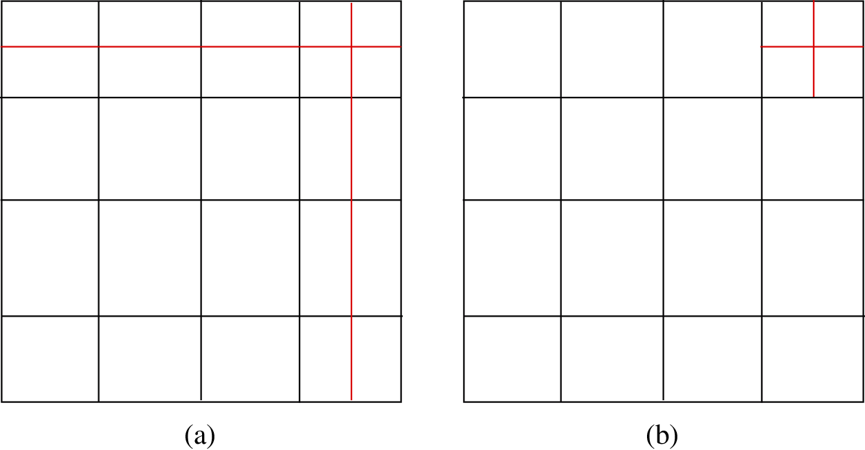
Figure 1: (a) NURBS global refinement and (b) expected local refinement
To address this problem, two approaches have been used in the literature. In [14], authors consider NURBS local prolongation operators which are based on multigrid principles. However, this approach needs to construct an operator by marking some extra elements for refinement, thereby, the resulting adaptive mesh is not the most efficient one. This situation can be partially alleviated by the use of hierarchical refinements of NURBS [15]. Another approach is to use splines with local refinement properties [14–19]. In authors’ opinion, the most commonly used splines with local refinement possibility are (truncated) hierarchical B-splines [20–23], T-splines [16,17], and PHT-splines (polynomial splines over hierarchical T-meshes) [18]. Because of a convenient local cross insertion and removal algorithm, we use PHT-splines in this study. PHT-splines have been used to solve static elastic solid issues. Numerical results show that the adaptive PHT refinement enjoys a higher convergence rate than uniform NURBS refinement [24]. However, since PHT-splines are polynomial functions, they are not able to exactly represent the geometry of shapes with conic sections, e.g., circles, ellipsoids, and spheres, which typically arise in engineering design and analysis. To tackle with this limitation, rational splines over hierarchical T-meshes (RHT-splines) have been recently introduced in [25]. Nevertheless, the continuity of RHT-splines is limited to only C1. Though the continuity of C1 is sufficient for the analysis of many engineering problems, for the description of geometry requiring higher continuity, RHT-splines will suffer from the geometry inexactness. To weaker this tight coupling between geometry and simulation, a new approach called Geometry-Independent Field approximaTion (GIFT) has been proposed [26]. This approach utilizes spline spaces for solution field independently of that for the geometry representation, and thus, offers the advantages of both the worlds. For instance, NURBS is used for the geometry representation (taken directly from the CAD model), and PHT-splines are use for the solution field. Thereby, the geometry information is preserved, and the local refinement is (independently) performed only on solution field. There are three main contributions of this article. (1) The GIFT method is employed to investigate the structural vibration based on the Kirchhoff plate theory. (2) In case of vibration, the advantage of GIFT is demonstrated with a feasible selection of spline domain of physical field. (3) Based on our established adaptive method for the vibration of thick plate problem [27], we extend to the adaptivity for thin plate vibration by sweeping the mode driven by a-posteriori error estimation, with the help of MAC method to recognize the correspondence between two different mesh spaces.
The organization of this paper is as follows. In Section 2, the variational form of linear elasto-dynamics, based on Kirchhoff plate theory, is set up. The weak form, based on IGA and GIFT framework, is introduced in Section 3. In Section 4, a-posteriori error estimation and the hierarchical local refinement process is developed. In Section 5, the a-posteriori error estimates and hierarchical local refinement of proposed in Section 4 is combined with MAC for modal analysis, and the resulting error-driven local adaptivity for vibration is presented. In Section 6, several numerical examples are presented. These results using GIFT approach show two major achievements: (1) Despite a poor geometric parameterization, an accurate numerical approximation can be obtained by adopting an appropriate parameterization in solution field. (2) When structural vibration is localized, the proposed adaptive refinement delivers a better convergence rate than the uniform refinement.
Let
where w is the deflection of the neutral plane of the plate in the z-direction. Thereby, w is the only independent variable, and we obtain a simple relationship
Moreover, the relationship between the three components of strain and the deflection is given by
By introducing the differential matrices
the relations (1) and (2) can be written as
Let C be the matrix of material stiffness constants. The in-plane (normal and shear) stresses σxx, σyy, and σxy can then be obtained, by substituting the value of
To evaluate the strain at the neutral plane of the plate, hence independent of the coordinate z, we introduce the pseudostrain
Let the parameter D = Eh312(1 − ν2) denote the bending stiffness of the plate, where E is the Young's modulus, and ν is the Poisson's ratio. Furthermore, let Mxx, Myy, and Mxy denote the bending moments, and twisting moments, respectively, which are defined as
These three components of the moments then define the pseudostress as
Let D denote the constant matrix of the material property and the plate thickness, which is defined as
For a thin plate, the generalized Hooke's law then gives the relation of pseudostress and pseudostrain as
Now let Vxz and Vyz denote the shear forces. Considering the moment equilibrium of the plate cell with respect to the x- (and y-) axis, and neglecting the second order small terms, leads to a relation in terms of moments
Let ρ denote the mass density of the plate material. The plate cell is then subjected to the inertial force
where bz is the external force. Using d Vxz = ∂ Vxz∂ x dx, and d Vyz = ∂ Vyz∂ y dy, we get
Substituting the relations of shear forces from (11), and the moments from (7), we get the following equation for homogeneous and isotropic plates
For free vibration analysis, with bz = 0, we get
We consider the clamped boundary conditions on all side, i.e.,
We now introduce the function space V0 = {v ∈ H2(ω) : v = ∂ v∂ n = 0 on γ }. Then the elasto-dynamic vibration problem in variational form reads [7,28]
where u is the displacement field,
3 The Discrete Form Using GIFT
Let P be the parametric domain. The physical domain ω is parametrized on P by a geometrical mapping F
We assume that the domain ω may consist sub-domains such that
where Ni1, i2, …, id(ɛ) can be a d-dimensional tensor product of NURBS, B-splines, T-splines, PHT-splines, etc. For brevity reasons, we introduce two sets of multi-indices (i1, i2, …, id) of NURBS basis functions by
Moreover, wherever suitable, for multi-index (i1, i2, …, id) we will interchangeably use the collapsed notation k Thence, Eqs. (17) and (18) are written as
In what follows, we will refer to the set
The GIFT method is presented in detail by Atroshchenko et al. [26]. In IGA, the solution field uI is represented through the same spline functions which are used for the geometry
where
where
Now, using the basis functions M k( ), we approximate the deflection w in Eq. (16) as
where M k(ɛ) are basis functions, and w kare unknown control variables. Substituting (25) in (16), we obtain the discrete form of the dynamical equation as follows:
where w denotes the vector of deflections at the control points, and K and M respectively denote the stiffness and mass matrices, which are defined as follows
where M xdenotes the basis functions from the space VG, and the matrix m the mass matrix
The general solution of the free vibration Eq. (26) can be expressed as
where i is the imaginary unit, is the eigenvector, and λ is the natural frequency. Substituting (29) into (26), and ignoring the virtual quantity, the natural frequency λ of thin plates can be calculated by solving the following generalized eigenproblem:
As eigenproblem (30) does not include the essential boundary conditions, it is necessary to find a proper way to impose essential boundary conditions. Some of the methods proposed in the literature to impose essential boundary conditions, e.g., [29,30] can be extended to the isogeometric framework. However, for efficiency reasons, we prefer another approach [31].
In this approach, simply supported boundary condition can be imposed through fixing the z-component of the first row of control variables for the respective boundary. Clamped boundary conditions can be imposed by fixing the z-component of the first two rows of control variables for the respective boundary.
In the next section, we introduce the error in the energy norm, and then define the hierarchical local refinement process. Unless otherwise stated, in what follows, we only compute the energy norm of the variables.
4 Hierarchical Local Refinement
For the complex cases, it is difficult to obtain the analytical solution for generalized eigenproblem (30). Therefore, to compute the errors in our numerical solution, we compute the solution on a refined mesh. This mesh is called the refined mesh, and the solution on it is called the better solution. Let
Now Let N denote the total number of elements in the domain. Then, the energy norm of error in the whole domain is defined as
Let η denote the error tolerance, i.e., if the error in any element is above this threshold, then the element is marked for refinement. For element marking, we employ the mean-value strategy with some simple modification. To be specific, we first select the elements for which the error satisfies
Thence, we mark the elements where
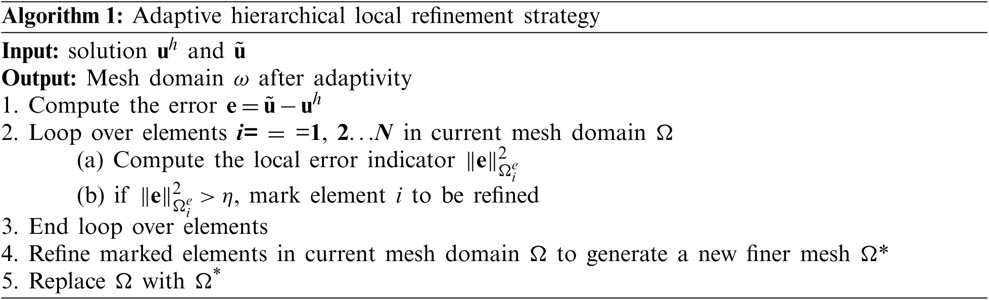
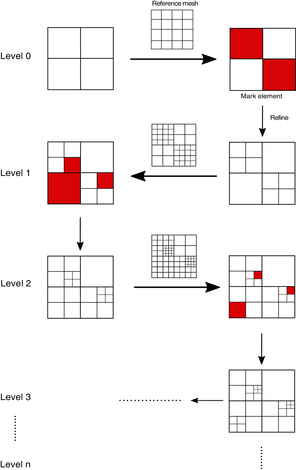
Figure 2: Adaptive refinement process of Algorithm 1 in 2D
5 Error-Driven Local Adaptivity for Vibration
In this section, error-driven local adaptivity based on the Algorithm 1 combined with MAC for vibration is presented. The purpose of our adaptive local refinement method for vibration is to get more accurate solution by less computing resources. Supposed that
wherein
Modal Assurance Criterion (MAC) is a statistical indicator originally proposed for orthogonality check [32] and has been developed as one of the most well-known method to compare modal vectors quantitatively [33]. In this paper, it is utilized for assistance for error estimation between two different mesh systems. The value of MAC is computed as the scalar product of the two sets of normalized eigenvectors
where ||⋅||m is the mass norm and defined by
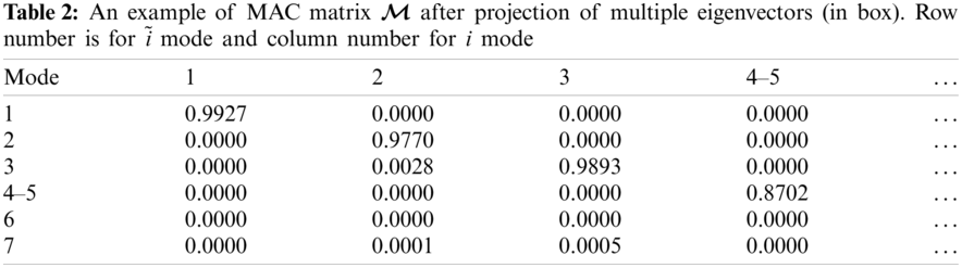
and m is the mass matrix defined in Eq. (28). The values of the MAC matrix are located in the interval [0, 1], where 0 means no consistent resemblance whereas 1 means a consistent correspondence. Generally, it is accepted that large values denote relatively consistent correlation whilst smaller value represents poor association of the two modal vectors. For instance, an example of MAC matrix
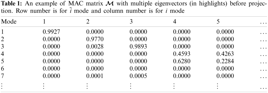
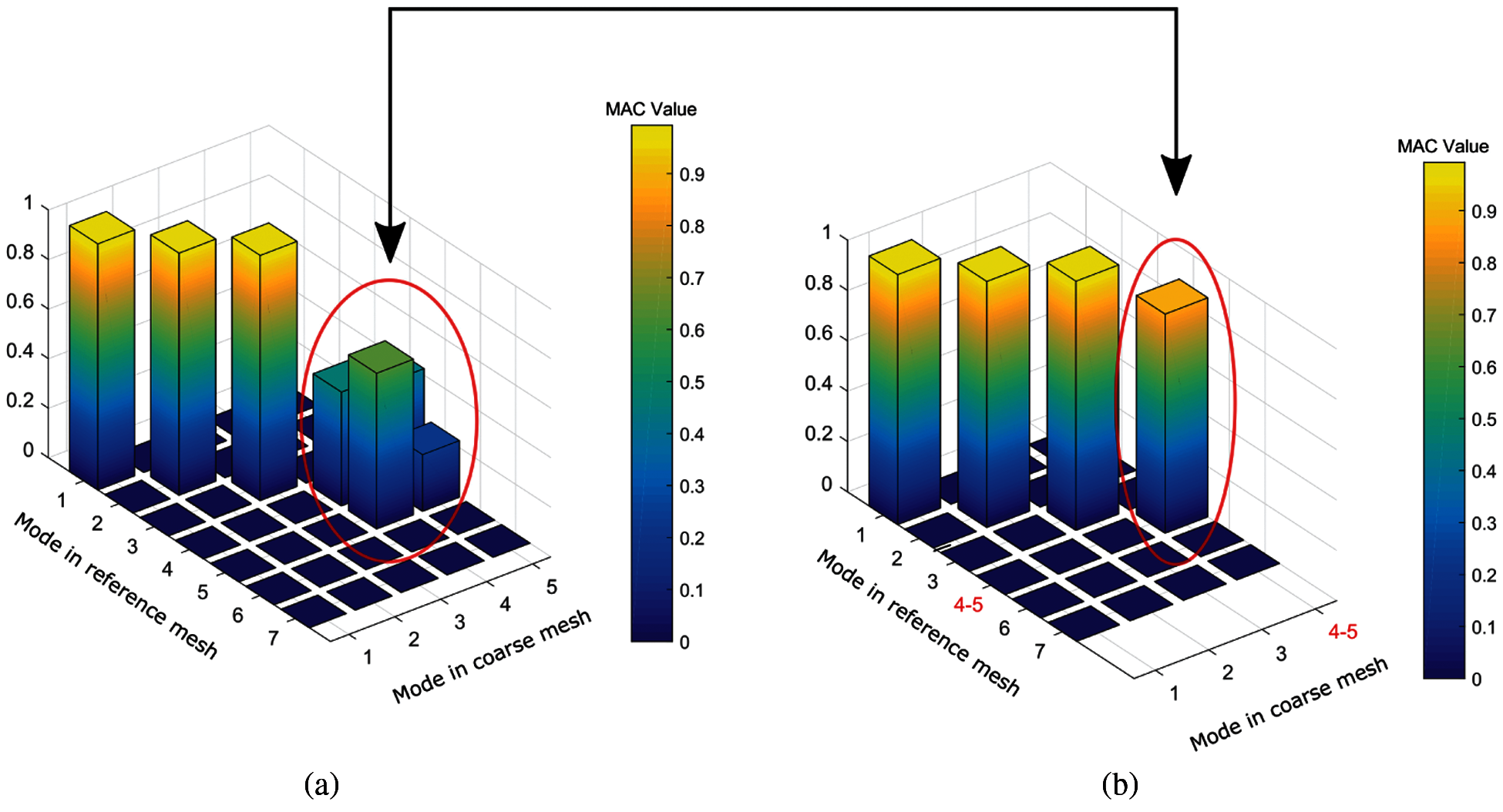
Figure 3: An example of 3D view for MAC values. (a) MAC matrix with multiple eigenvectors (in red circle) before projection; (b) MAC matrix after projection of multiple eigenvectors (in red circle)
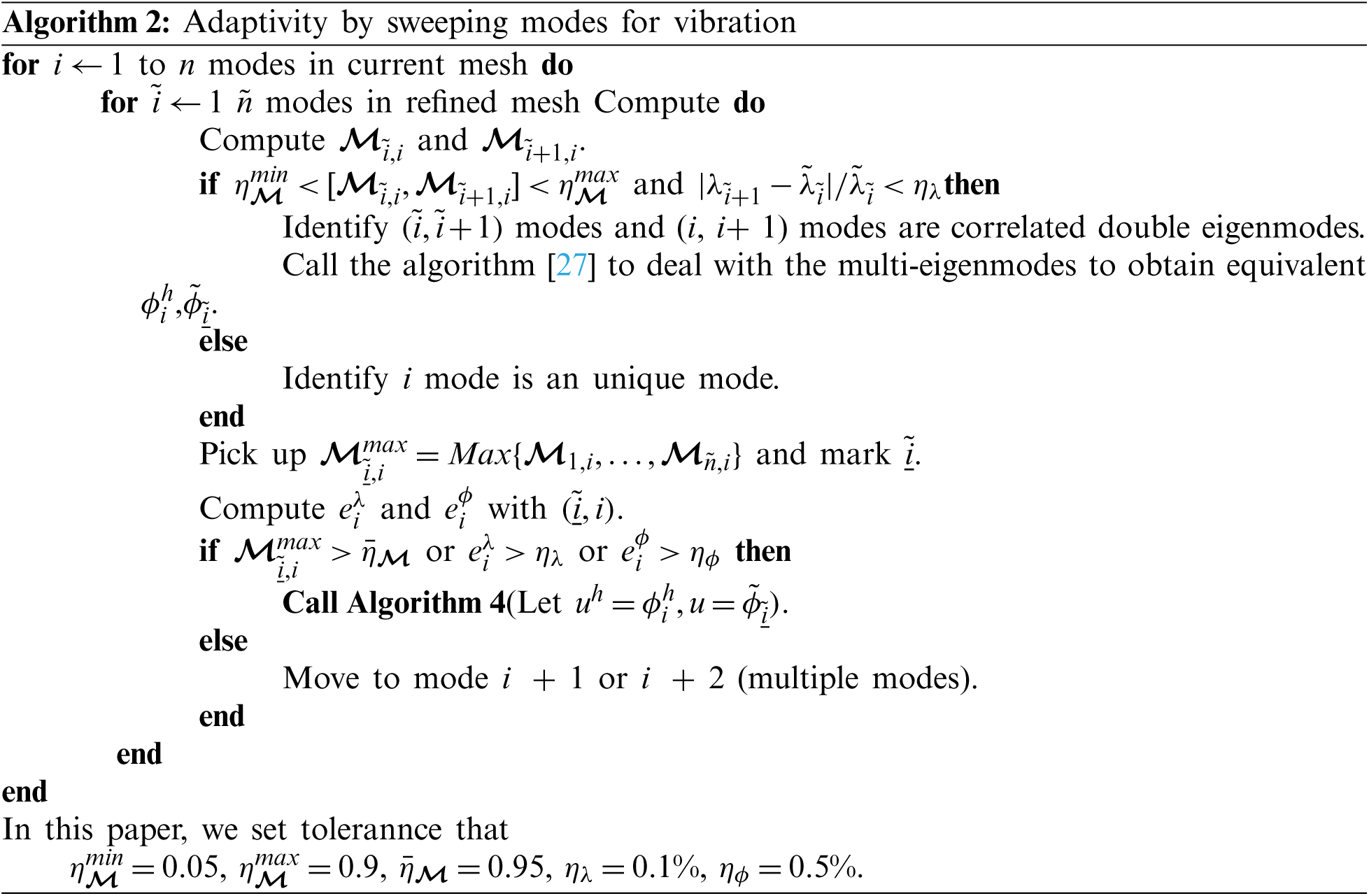
5.2 Adaptive Local Refinement for Vibration
As we know, mode shapes of structural vibration are often different from modes to modes. One may pay attention to the mode shapes around specific range of frequency according to engineering problems. For general applications, in this paper, the adaptive refinement is carried out via sweeping modes from low to high frequency. The procedure is summarized in Algorithm 2.
Four numerical examples are carried out for the following purposes. Example in Section 6.1 is the vibration investigation of circular plate to show that GIFT method has the merit of flexibility to choose spline space in solution field independently from that of geometry, which would yield better solution compared to IGA on condition that control points describing geometry are distributed unreasonably. Examples in Sections 6.2–6.4 employ GIFT, with NURBS representing geometry and PHT describing solution field, to study vibration problem for heterogeneous plate with different shapes, especially, analysis of multiple modes is presented in example in Section 6.2. These heterogeneous plate perform obvious concentrated local response where PHT is able to show the advantage of local refinement. Noted that in instances of Sections 6.2–6.4, due to lack of theoretical solution for the problems, we adopt the computational result from the very fine uniform mesh as the approximation of analytical solution.
The geometric and material parameters for circular plate are listed in Table 3, with radius R, thickness h, Young's modulus E, and density ρ. On assumption that the geometry of circular plate is established by cubic NURBS basis functions with irregularly distributed control points 24 × 24, shown in Fig. 4a. In IGA scheme, the solution space in Fig. 4b is imposed to be the same as geometric space. However, GIFT is free to pick up the solution space so that the uniform one in Fig. 4c is preferred here. For better comparing with theoretical results [34], the normalized natural frequency related parameter
where λ is natural frequency and D is flexural stiffness. Consequently, supposed that
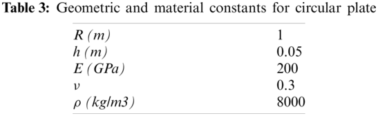
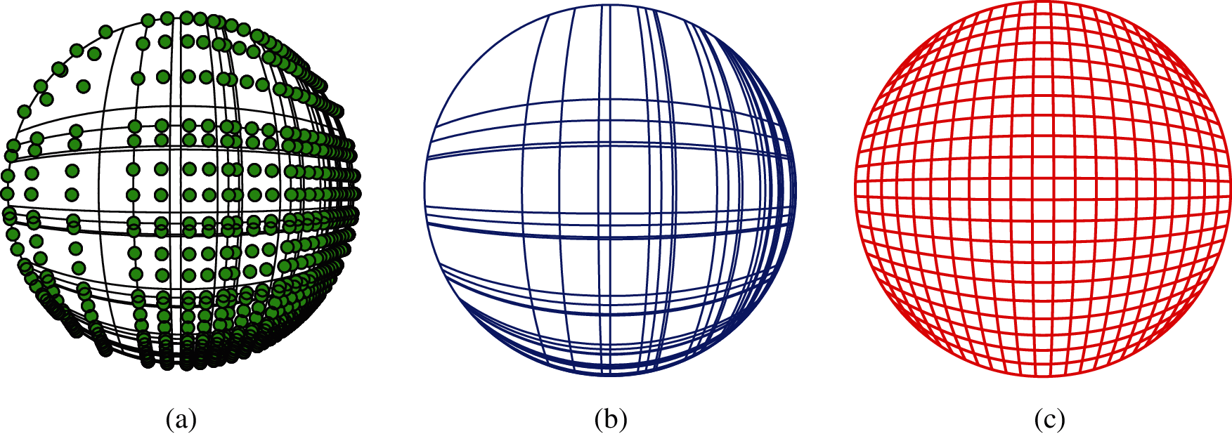
Figure 4: The same geometry parameterization and different spline spaces in solution field of IGA and GIFT for circular plate. Cubic NURBS for both IGA and GIFT. (a) Geometry with 24 × 24 control points; (b) Geometry with 24 × 24 control points; (c) Geometry with 24 × 24 control points
In this example, IGA and GIFT method is compared with exact solution in simply supported boundary condition and clamped boundary condition separately, where the difference of these two boundary conditions has been clarified in Section 3.1. The results are illustrated in Tables 4, 5 and Fig. 5. It is observed that GIFT shows a better accuracy than IGA with increasing of modes. This example inspires us that when the geometric space of structure is not good enough, we can count on GIFT to re-construct the solution space to achieve a better precision.
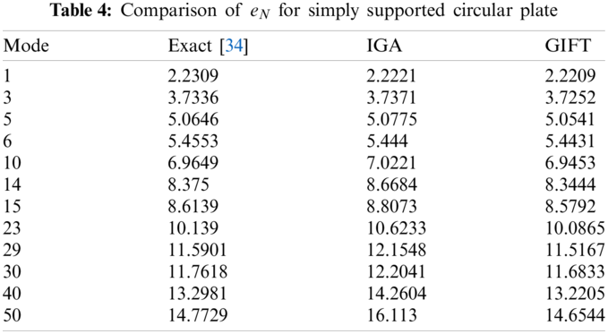
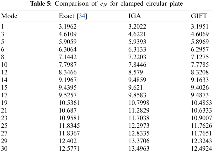
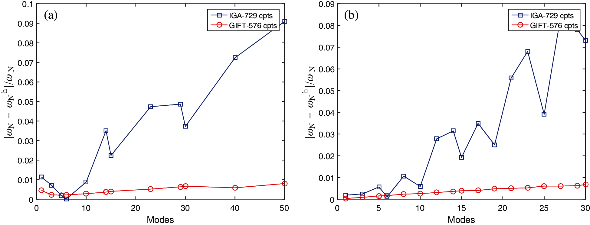
Figure 5: Comparison of eN between IGA (729 control points) and GIFT (576 control points) in solution field (Cubic NURBS, cpts control points). (a) Simply support; (b) clamped
6.2 Heterogeneous L-Shape Plate
In this test, a heterogeneous L-shape structure is built with 3 Patches where relevant geometric parameters and material constants are displayed in Fig. 6a. The whole domain boundary is simply supported. Density ρ is 2700, and thickness h is 0.01 and Poisson's rate ν is 0.3. The Young's modulus of 3 Patches is E2 = E = 107, E1 = E3= 1000E2 respectively so that it is evident the vibration would be concentrated in the Patch 2 as the material is softest in this area. As explicitly discussed on the principle in Section 5, the adaptivity starts with an initial mesh in Fig. 7a from the 1th mode and afterwards sweeps from low to high frequency. Here we would like to emphasize that firstly, the error indicators of both natural frequency
where
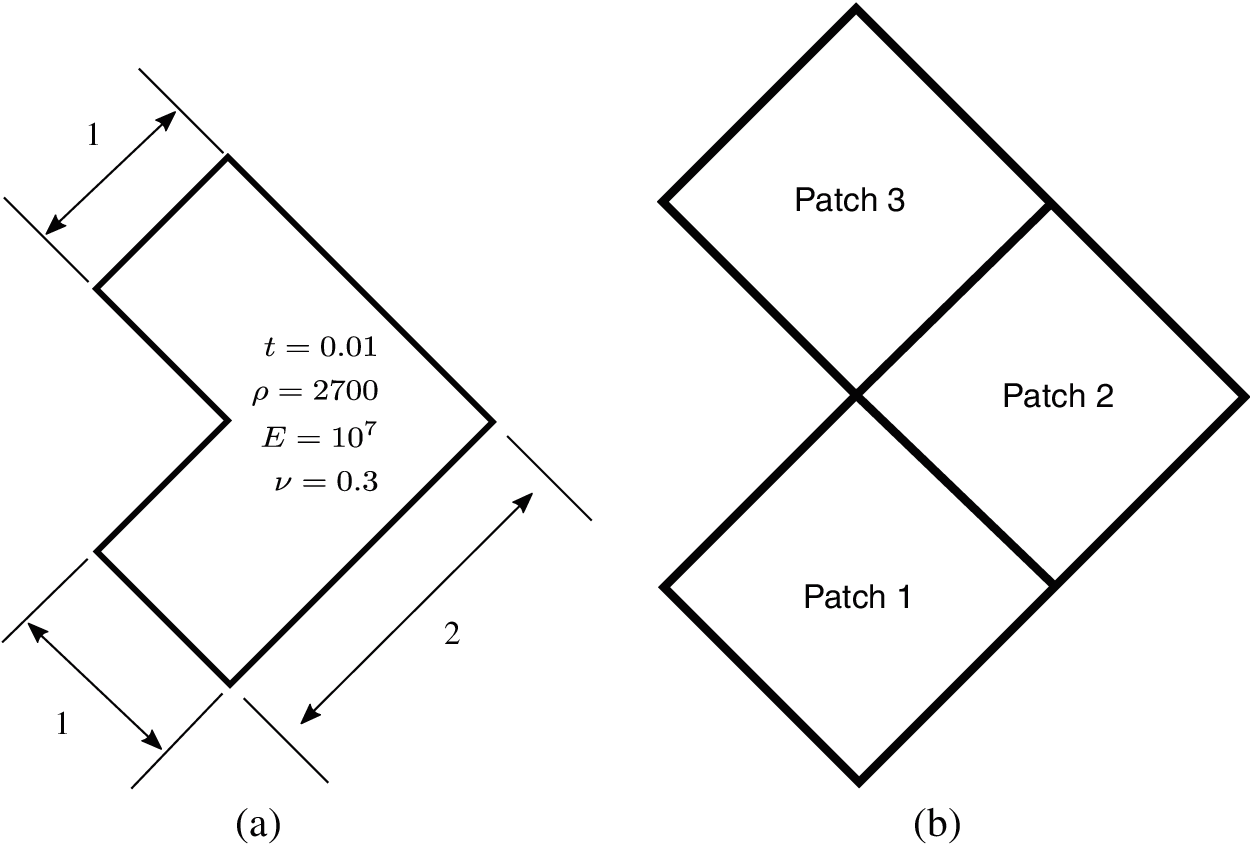
Figure 6: A simply supported heterogeneous L-shape plate: (a) geometric parameters and (b) discretization of patches,
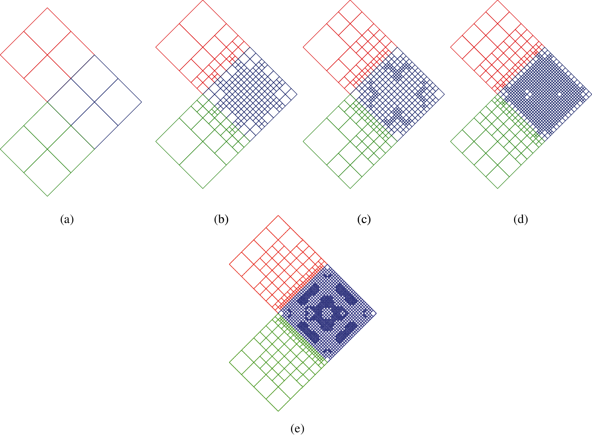
Figure 7: Adaptive refinement process of 1–15th mode for vibration of L-shape plate. Especially, 2–3th, 5–6th, 7–8th, 9–10th, 12–13th, 14–15th modes are multiple modes. Geometry-NURBS with order p1 = 1, p2 = 1; Solution Field-PHT with order q1 = 3, q2 = 3. (a) Initial mesh; (b) Adaptive mesh for 1th mode; (c) Adaptive mesh for 2–3, 4th mode; (d) Adaptive mesh for 5–6, 7–8th mode; (e) Adaptive mesh for 9–10, 11, 12–13, 14–15th mode
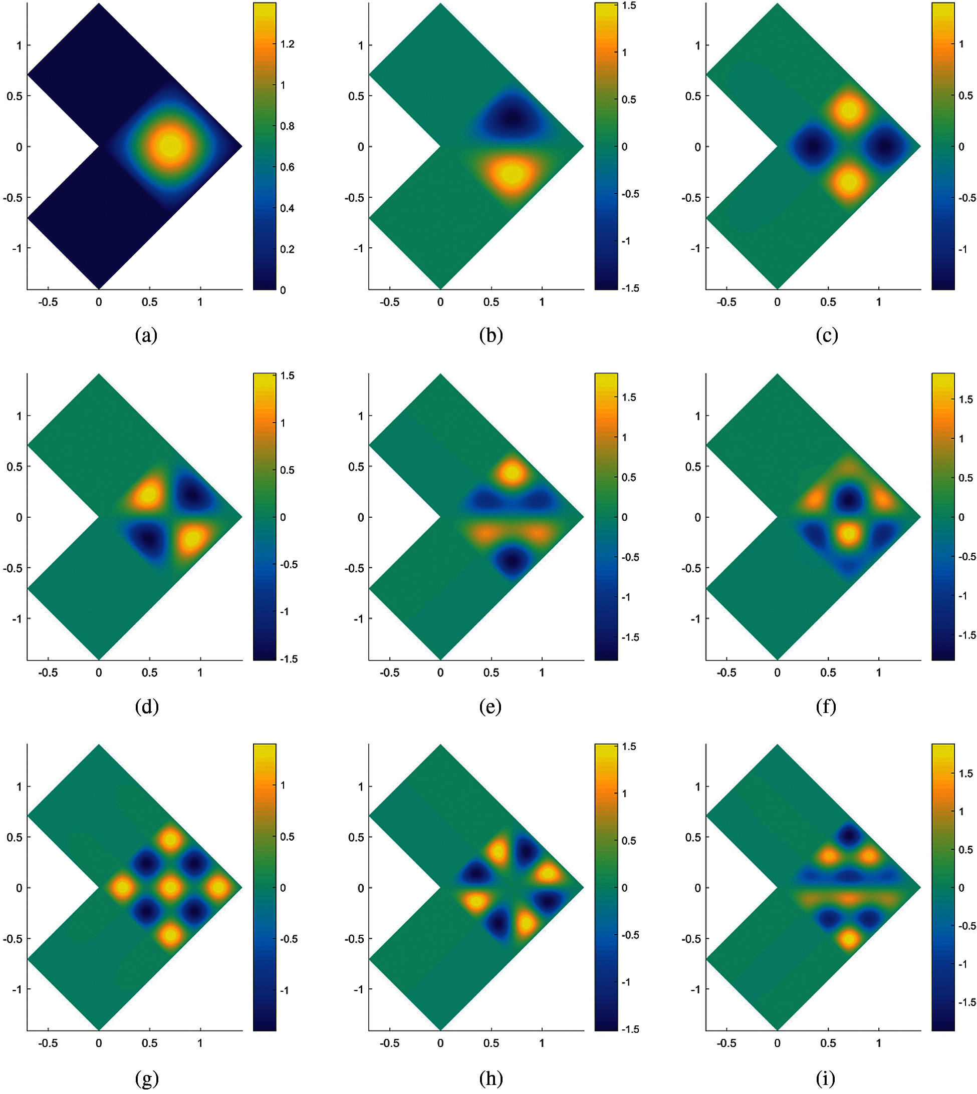
Figure 8: Mode shapes 1–15th of L-shape plate, where
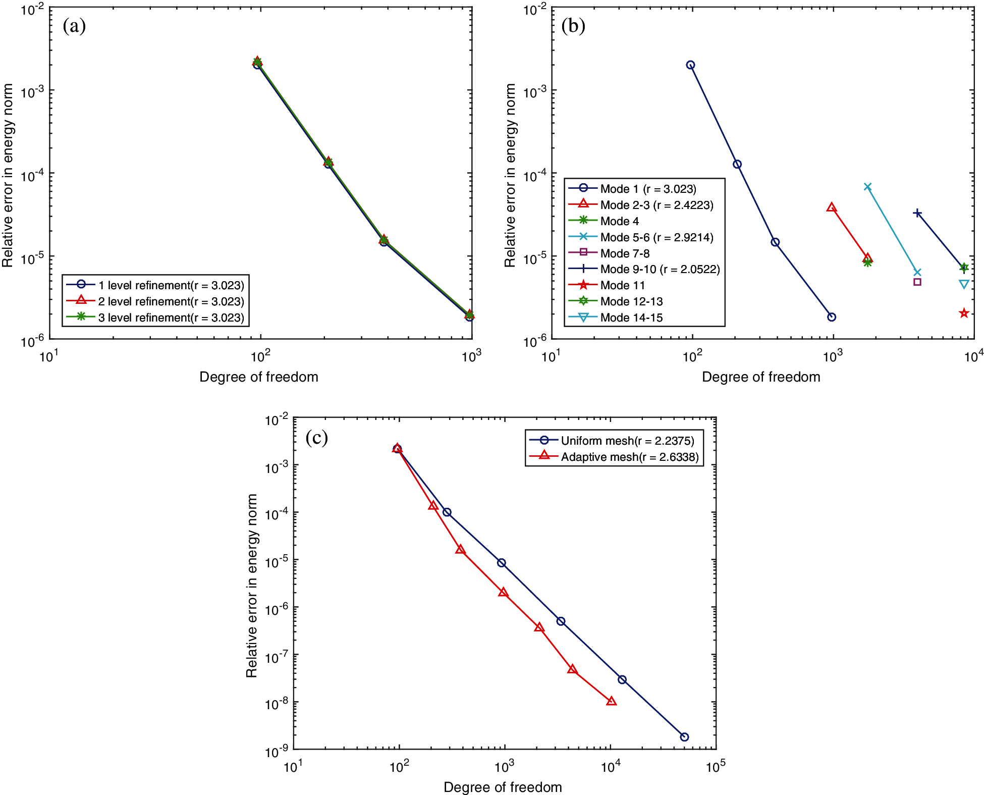
Figure 9: (a) Comparisons of error indicator of natural frequency at 1th mode
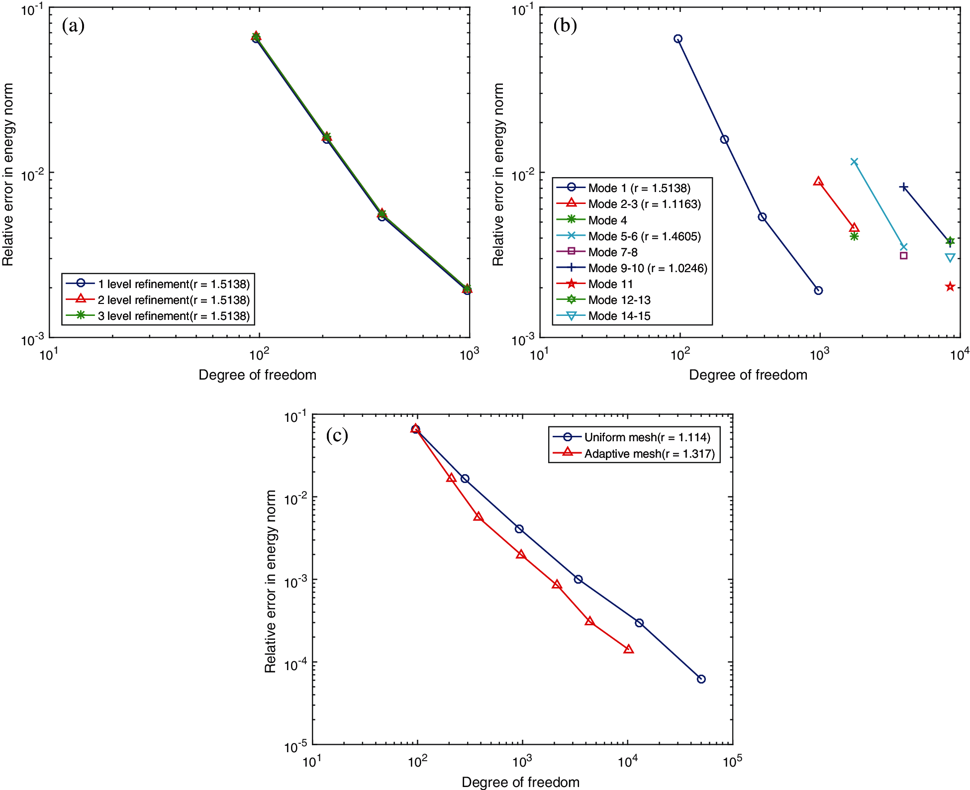
Figure 10: (a) Comparisons of error indicator of eigenvector at 1th mode
6.3 Heterogeneous Plate with a Hole
In this section, a plate with a hole where the boundary simply supported is shown in Fig. 11, consisting of two material Patches with E1 = E = 109, E2 = 100E1. Density ρ is 2700, and thickness h is 0.01 and Poisson’s rate ν is 0.3. Consequently, the vibration response and local adaptive refinement is undoubtedly centralized in the Patch 2 area, seen in Figs. 12 and 13. Different from L-shape example in Section 6.2, the geometry of the hole is non-linear so that cross-derivative of the parametrization in Eq. (16) are non-zero, which is a good opportunity to validate our algorithm is available in terms of non-linear mapping as well. The convergence rate plot of error indicators in both of Figs. 14a and 15a support the reasonability of adopting refinement level Le = 1 for reference parametrization in solution field. Without any surprise, adaptive refinement performs a higher convergence rate than uniform refinement, based on an approximation of solution by a very fine mesh with 132,870 dof.
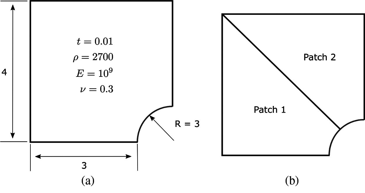
Figure 11: A simply supported heterogeneous platehole: (a) geometric parameters and (b) discretization of patches, E1 = E, E2 = 100E1
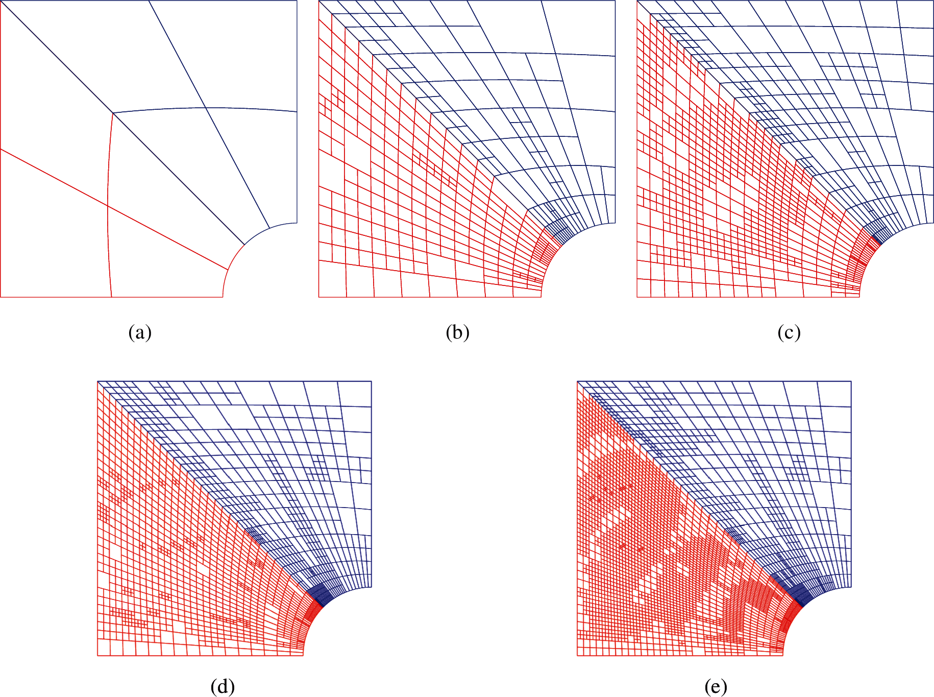
Figure 12: Adaptive refinement process of 1–9th mode for vibration of platehole. Geometry-NURBS with order p1 = 1, p2 = 2; Solution Field-PHT with order q1 = 3, q2 = 3
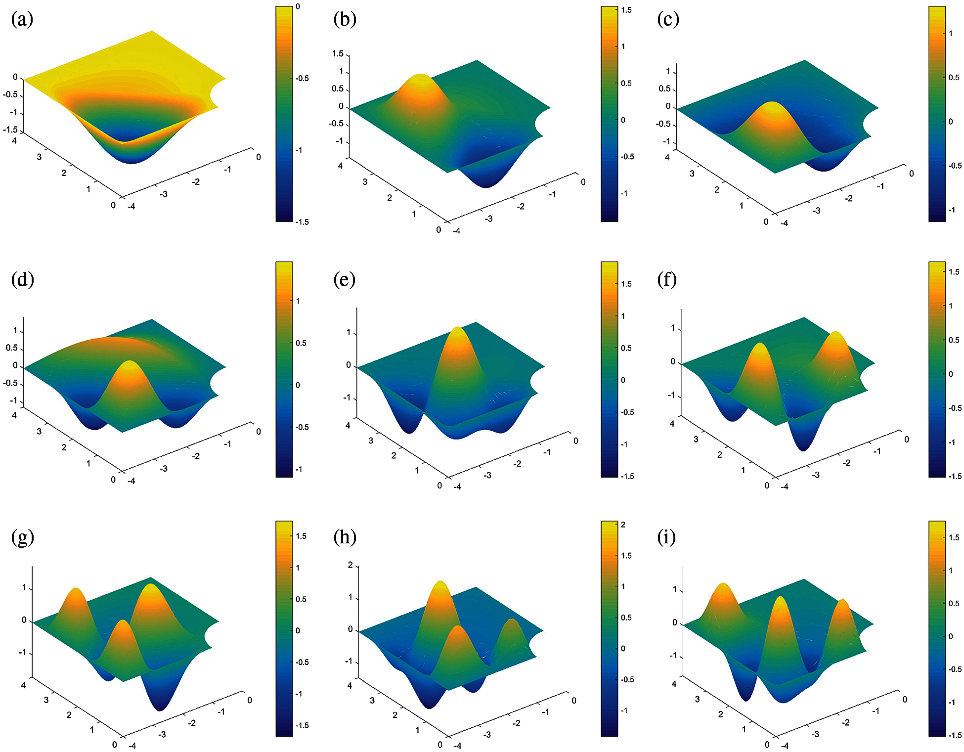
Figure 13: Mode shapes 1–9th of platehole, where
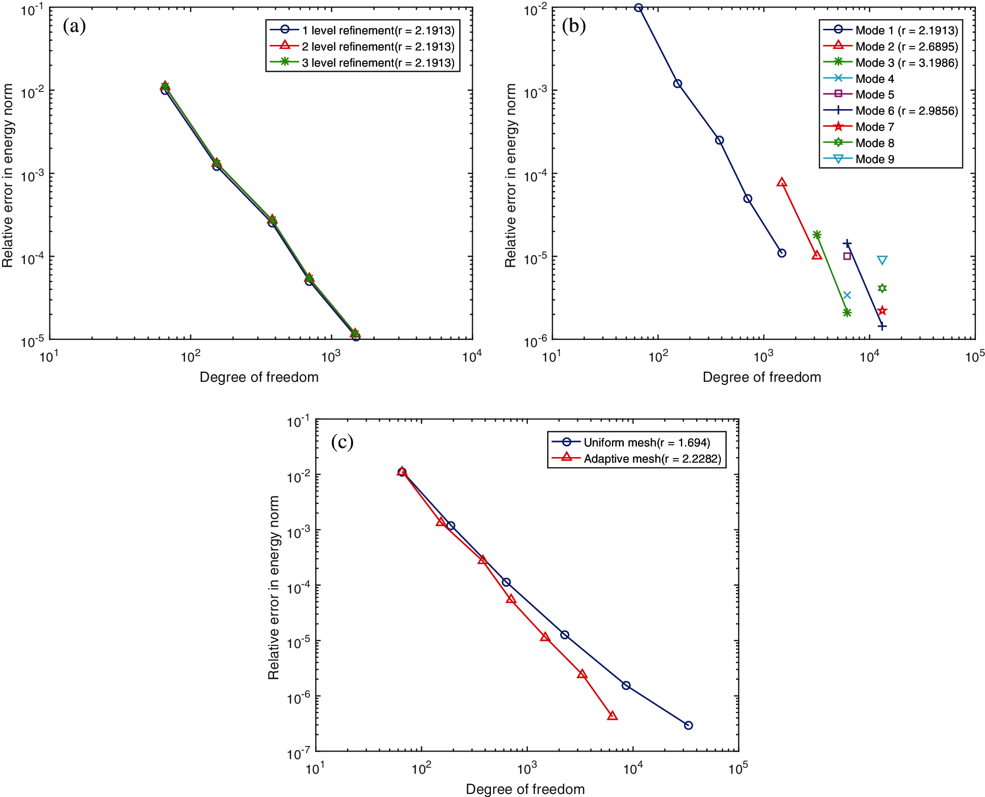
Figure 14: (a) Comparisons of
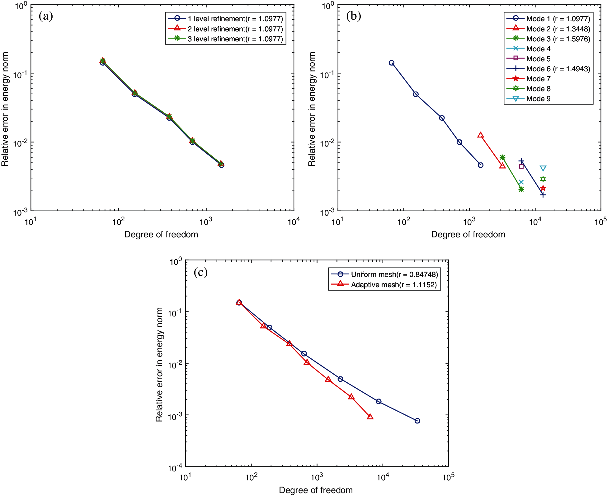
Figure 15: (a) Comparisons of
6.4 Heterogeneous Lshaped-Bracket
The L-shape bracket is such a complex structure that it is divided into 18 Patches in Fig. 16b. Patches 1–4 are softer than other Patches that E1 − 4 = E, E5 − 18 = 100E = 109. Density ρ is 2700, and thickness h is 0.01 and Poisson's rate ν is 0.3. The whole boundary including the 4 holes is imposed to be simply supported except the right edge marked with red colour in Fig. 16a, where the boundary condition is assumed to be free. It is intended to make the vibration around Patch 4 is more fiercely than other parts. As a consequence, at the first 5 modes (1th–5th), the structural vibration and adaptive local refinement merge into Patches 1–4. When it comes to the 6th mode, the mode shape moves to the middle of structure (Patch 9, 10), seen in Fig. 18f. It induces the rise of the error (proved by plot of Mode 6 in Figs. 19b and 20b, respectively in this district and certainly the adaptive refinement will locate nearby, seen in Fig. 17e. After that, the modal shape moves back to Patches 1–4 and the adaptivity keeps going on in that zone. The convergence rate between adaptive refinement and uniform refinement are computed upon the basis of an approximate solution with 301,470 dof. Apparently, in Figs. 19c and 20, the convergence rate of adaptive refinement is much steeper (more than twice) than that of uniform refinement. This indicates the structural response is much local in this problem.
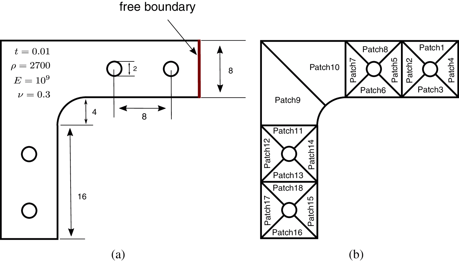
Figure 16: A simply supported with right free boundary heterogeneous Lshaped-bracket: (a) geometric parameters and (b) discretization of patches, E1 − 4 = E, E5 − 18 = 100E
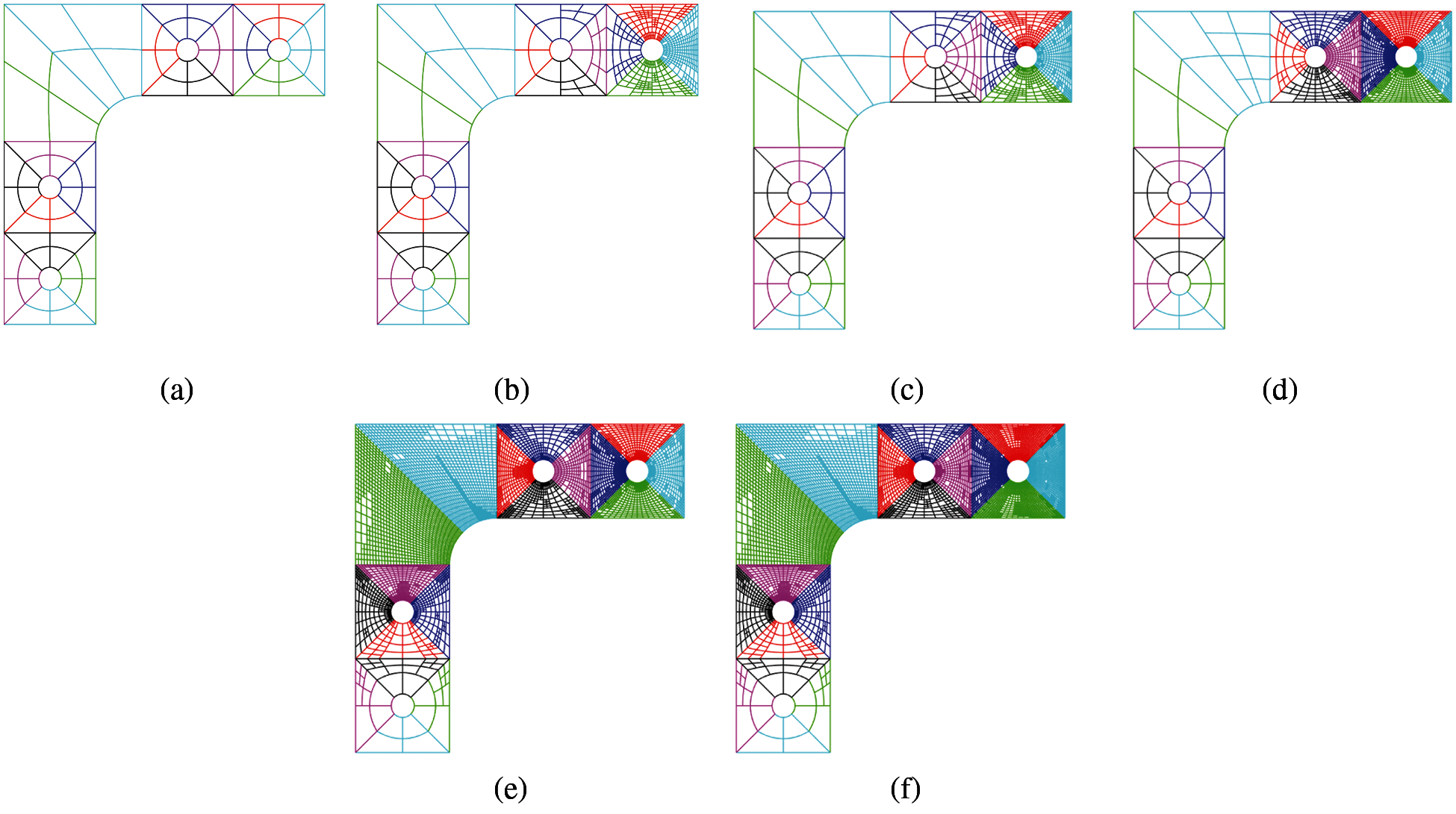
Figure 17: Adaptive refinement process of 1–9th mode for vibration of Lshaped-bracket. Geometry-NURBS with order p1 = 1, p2 = 2; Solution Field-PHT with order q1 = 3, q2 = 3. (a) Initial mesh; (b) Adaptive mesh for 1th mode; (c) Adaptive mesh for 2th mode; (d) Adaptive mesh for 3, 4, 5th mode; (e) Adaptive mesh for 6, 7th mode; (f) Adaptive mesh for 8, 9th mode
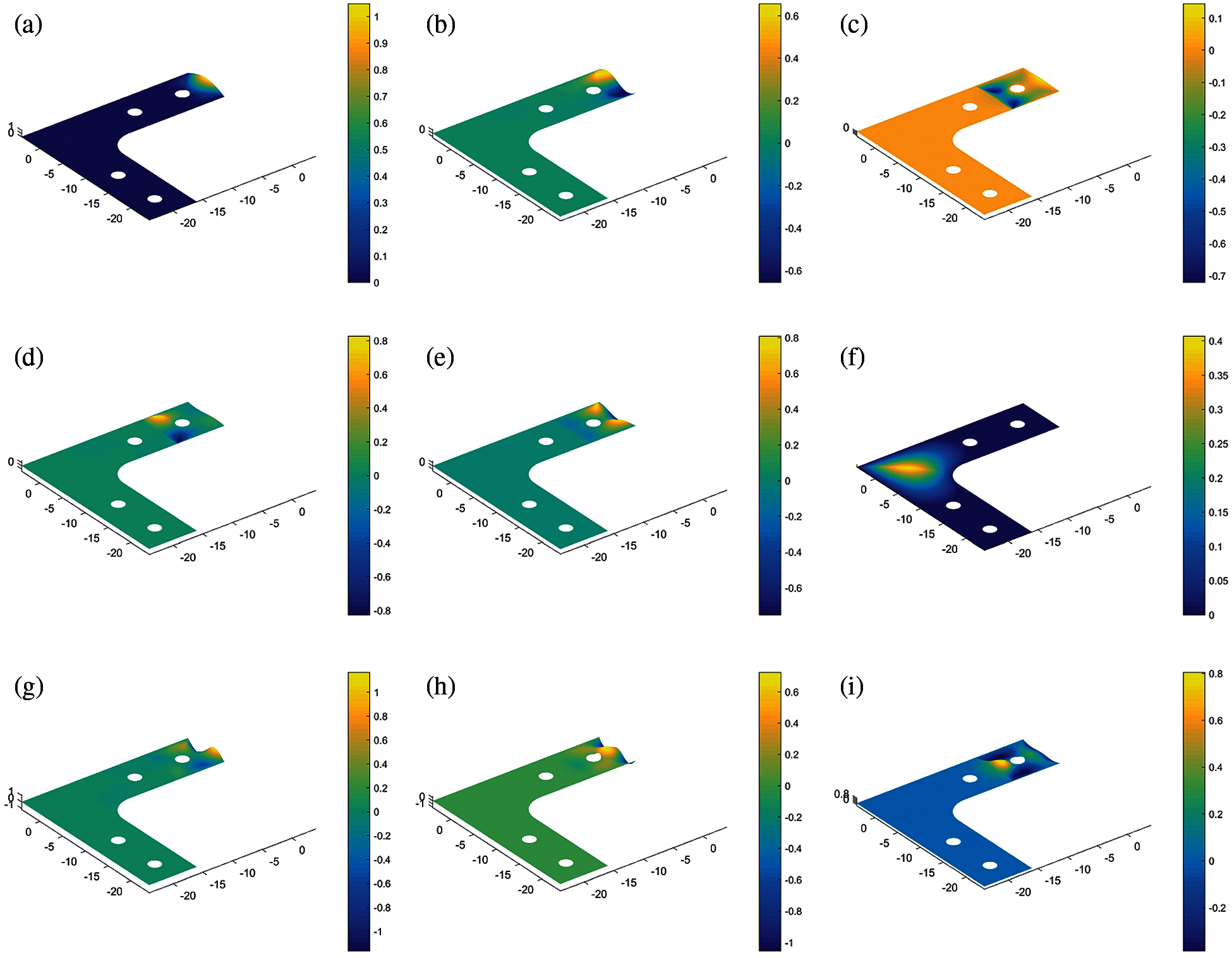
Figure 18: Mode shapes 1–9th of Lshaped-bracket, where
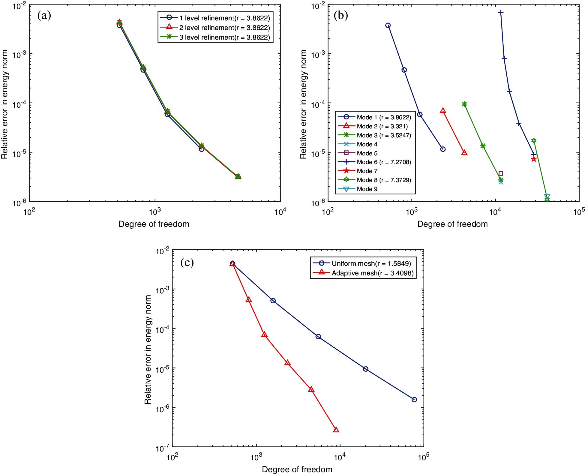
Figure 19: (a) Comparisons of
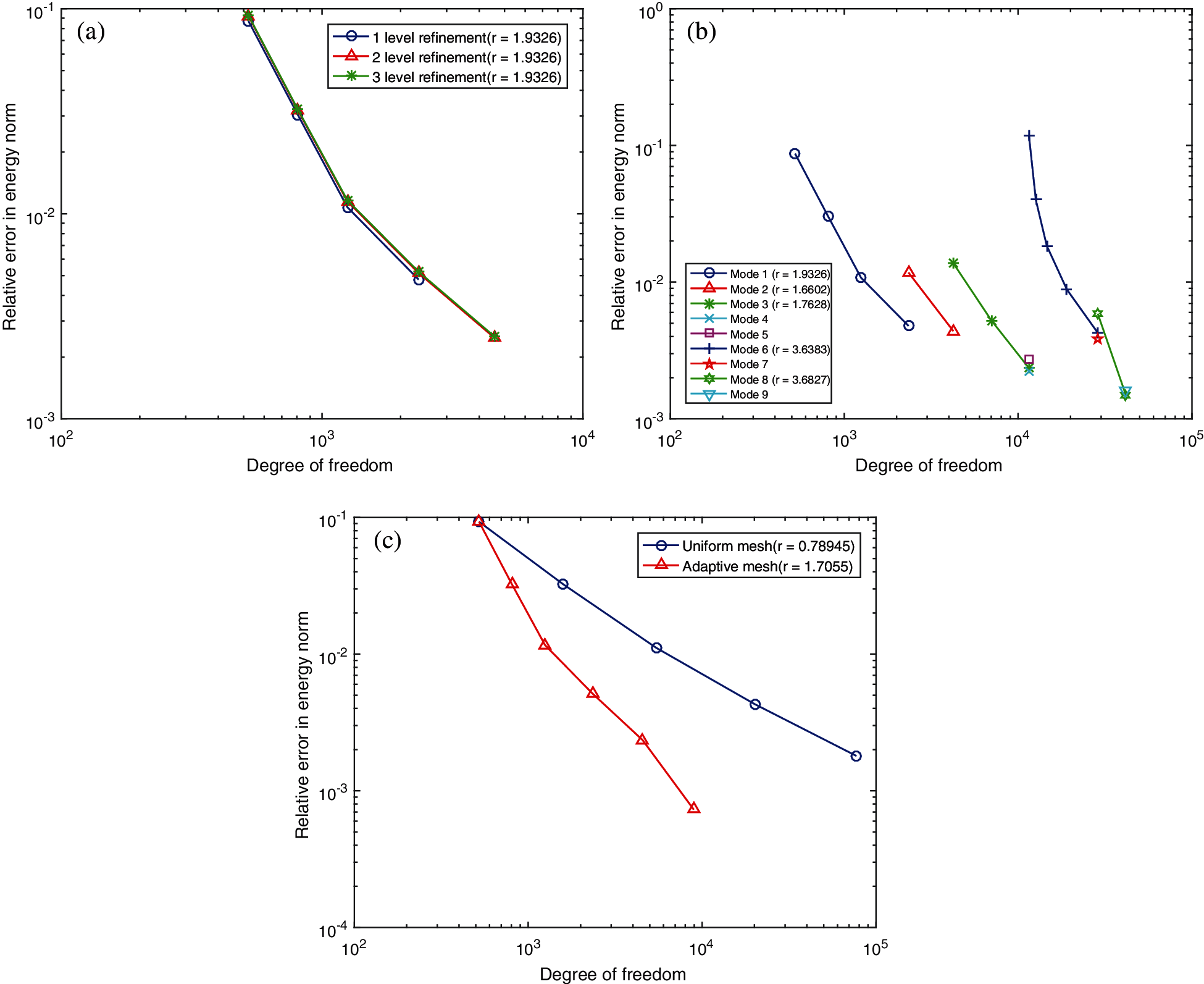
Figure 20: (a) Comparisons of error indicator of eigenvector at 1th mode
In this article, based on our proposed adaptivity strategy in the framework of GIFT paradigm utilized for vibration of Reissner–Mindlin plate, it is developed to investigate the error-driven adaptivity for structural vibration of Kirchhoff plate. GIFT offers us the convenience to choose solution field independently from geometry so that the good accuracy can be achieved by better approximation in the solution field even though the geometric parameterization is not fairly designed as supported by the example in Section 6.1. Furthermore, it allows us to connect NURBS describing for geometry with PHT represented for solution field to reserve geometric precision and realize local refinement. Besides, when dealing with error estimation process, MAC scheme is helpful to locate the correspondence of modal vectors covering multiple eigenvectors between two different meshes. Our error indicator is proved to be reasonably chosen and the proposed adaptive strategy shows a better convergence rate than uniform refinement, supported by numerical tests in Sections 6.2–6.4.
We believe the proposed algorithm has potential to be practical in engineering problems. The developed method is available to precisely describe complex geometry of structure and simultaneously saves computational resource for given accuracy, especially for structures with local mechanical behaviour. As to the adaptivity of vibration by sweeping modes from low to high frequency, this adaptive strategy can be started from any mode or used to optimize some specific modes people are interested in. It would be productive to modal analysis for vibration problem. In the future, we intend to extend this method to 3D elasto-dynamics including the space-time problems.
Acknowledgement: This study was funded by Research Grant for 100 Talents of Guangxi Plan, The Starting Research Grant for High-Level Talents from Guangxi University, Generalized Isogeometric Analysis with Homogeniztion Theory for Soft Acoustic Metamaterials (20200312), Science and Technology Major Project of Guangxi Province (AA18118055), Guangxi Natural Science Foundation (2018JJB160052), and Application of Key technology in Building Construction of Prefabricated Steel Structure (BB30300105).
Funding Statement: This study was funded by Natural Science Foundation of China (Grant No. 12102095), Research grant for 100 Talents of Guangxi Plan, The Starting Research Grant for High-Level Talents from Guangxi University, Generalized Isogeometric Analysis with Homogeniztion Theory for Soft Acoustic Metamaterials (AD20159080), Science and Technology Major Project of Guangxi Province (AA18118055), Guangxi Natural Science Foundation (2018JJB160052), and Application of Key Technology in Building Construction of Prefabricated Steel Structure (BB30300105).
Conflicts of Interest: The authors declare that they have no conflicts of interest to report regarding the present study.
1. Hughes, T. J., Cottrell, J. A., Bazilevs, Y. (2005). Isogeometric analysis: CAD, finite elements, nurbs, exact geometry and mesh refinement. Computer Methods in Applied Mechanics and Engineering, 194(39), 4135–4195. DOI 10.1016/j.cma.2004.10.008. [Google Scholar] [CrossRef]
2. Nguyen, V. P., Anitescu, C., Bordas, S. P., Rabczuk, T. (2015). Isogeometric analysis: An overview and computer implementation aspects. Mathematics and Computers in Simulation, 117, 89–116. DOI 10.1016/j.matcom.2015.05.008. [Google Scholar] [CrossRef]
3. Lian, H., Kerfriden, P., Bordas, S. P. (2016). Implementation of regularized isogeometric boundary element methods for gradient-based shape optimization in two-dimensional linear elasticity. International Journal for Numerical Methods in Engineering, 106(12), 972–1017. DOI 10.1002/nme.5149. [Google Scholar] [CrossRef]
4. Lian, H., Kerfriden, P., Bordas, S. (2017). Shape optimization directly from cad: An isogeometric boundary element approach using T-splines. Computer Methods in Applied Mechanics and Engineering, 317, 1–41. DOI 10.1016/j.cma.2016.11.012. [Google Scholar] [CrossRef]
5. Chen, L., Lian, H., Liu, Z., Chen, H., Atroshchenko, E. et al. (2019). Structural shape optimization of three dimensional acoustic problems with isogeometric boundary element methods. Computer Methods in Applied Mechanics and Engineering, 355, 926–951. DOI 10.1016/j.cma.2019.06.012. [Google Scholar] [CrossRef]
6. Cottrell, J. A., Reali, A., Bazilevs, Y., Hughes, T. J. (2006). Isogeometric analysis of structural vibrations. Computer Methods in Applied Mechanics and Engineering, 195(41–43), 5257–5296. DOI 10.1016/j.cma.2005.09.027. [Google Scholar] [CrossRef]
7. Shojaee, S., Izadpanah, E., Valizadeh, N., Kiendl, J. (2012). Free vibration analysis of thin plates by using a NURBS-based isogeometric approach. Finite Elements in Analysis and Design, 61, 23–34. DOI 10.1016/j.finel.2012.06.005. [Google Scholar] [CrossRef]
8. del Toro Llorens, A., Kiendl, J. (2021). An isogeometric finite element-boundary element approach for the vibration analysis of submerged thin-walled structures. Computers & Structures, 256, 106636. DOI 10.1016/j.compstruc.2021.106636. [Google Scholar] [CrossRef]
9. Patton, A., Antolin, P., Dufour, J. E., Kiendl, J., Reali, A. (2021). Accurate equilibrium-based interlaminar stress recovery for isogeometric laminated composite kirchhoff plates. Composite Structures, 256, 112976. DOI 10.1016/j.compstruct.2020.112976. [Google Scholar] [CrossRef]
10. Sobota, P. M., Dornisch, W., Müller, R., Klinkel, S. (2017). Implicit dynamic analysis using an isogeometric reissner–mindlin shell formulation. International Journal for Numerical Methods in Engineering, 110(9), 803–825. DOI 10.1002/nme.5429. [Google Scholar] [CrossRef]
11. Thai, C. H., Nguyen-Xuan, H., Nguyen-Thanh, N., Le, T. H., Nguyen-Thoi, T. et al. (2012). Static, free vibration, and buckling analysis of laminated composite reissner–mindlin plates using nurbs-based isogeometric approach. International Journal for Numerical Methods in Engineering, 91(6), 571–603. DOI 10.1002/nme.4282. [Google Scholar] [CrossRef]
12. van Do, V. N., Lee, C. H. (2021). Isogeometric layerwise formulation for bending and free vibration analysis of laminated composite plates. Acta Mechanica, 232(4), 1329–1351. DOI 10.1007/s00707-020-02900-7. [Google Scholar] [CrossRef]
13. Shafei, E., Faroughi, S., Rabczuk, T. (2021). Nonlinear transient vibration of viscoelastic plates: A NURBS-based isogeometric HSDT approach. Computers & Mathematics with Applications, 84, 1–15. DOI 10.1016/j.camwa.2020.12.006. [Google Scholar] [CrossRef]
14. Chemin, A., Elguedj, T., Gravouil, A. (2015). Isogeometric local h-refinement strategy based on multigrids. Finite Elements in Analysis and Design, 100, 77–90. DOI 10.1016/j.finel.2015.02.007. [Google Scholar] [CrossRef]
15. Schillinger, D., Dede, L., Scott, M. A., Evans, J. A., Borden, M. J. et al. (2012). An isogeometric design-through-analysis methodology based on adaptive hierarchical refinement of NURBS, immersed boundary methods, and T-spline CAD surfaces. Computer Methods in Applied Mechanics and Engineering, 249, 116–150. DOI 10.1016/j.cma.2012.03.017. [Google Scholar] [CrossRef]
16. Sederberg, T. W., Cardon, D. L., Finnigan, G. T., North, N. S., Zheng, J. et al. (2004). T-spline simplification and local refinement. ACM Transactions on Graphics, 23(3), 276–283. DOI 10.1145/1015706.1015715. [Google Scholar] [CrossRef]
17. Bazilevs, Y., Calo, V. M., Cottrell, J. A., Evans, J. A., Hughes, T. J. R. et al. (2010). Isogeometric analysis using T-splines. Computer Methods in Applied Mechanics and Engineering, 199(5–8), 229–263. DOI 10.1016/j.cma.2009.02.036. [Google Scholar] [CrossRef]
18. Deng, J., Chen, F., Li, X., Hu, C., Tong, W. et al. (2008). Polynomial splines over hierarchical T-meshes. Graphical Models, 70(4), 76–86. DOI 10.1016/j.gmod.2008.03.001. [Google Scholar] [CrossRef]
19. Kang, H., Xu, J., Chen, F., Deng, J. (2015). A new basis for PHT-splines. Graphical Models, 82, 149–159. DOI 10.1016/j.gmod.2015.06.011. [Google Scholar] [CrossRef]
20. Forsey, D. R., Bartels, R. H. (1988). Hierarchical B-spline refinement. Proceedings of the 15th Annual Conference on Computer Graphics and Interactive Techniques, New York, USA. [Google Scholar]
21. Vuong, A. V., Giannelli, C., Jüttler, B., Simeon, B. (2011). A hierarchical approach to adaptive local refinement in isogeometric analysis. Computer Methods in Applied Mechanics and Engineering, 200(49–52), 3554–3567. DOI 10.1016/j.cma.2011.09.004. [Google Scholar] [CrossRef]
22. Giannelli, C., Jüttler, B., Speleers, H. (2012). THB-splines: The truncated basis for hierarchical splines. Computer Aided Geometric Design, 29(7), 485–498. DOI 10.1016/j.cagd.2012.03.025. [Google Scholar] [CrossRef]
23. Giannelli, C., Jüttler, B., Kleiss, S., Mantzaflaris, A., Simeon, B. et al. (2016). THB-splines: An effective mathematical technology for adaptive refinement in geometric design and isogeometric analysis. Computer Methods in Applied Mechanics and Engineering, 299, 337–365. DOI 10.1016/j.cma.2015.11.002. [Google Scholar] [CrossRef]
24. Nguyen-Thanh, N., Nguyen-Xuan, H., Bordas, S. P. A., Rabczuk, T. (2011). Isogeometric analysis using polynomial splines over hierarchical t-meshes for two-dimensional elastic solids. Computer Methods in Applied Mechanics and Engineering, 200(21–22), 1892–1908. DOI 10.1016/j.cma.2011.01.018. [Google Scholar] [CrossRef]
25. Nguyen-Thanh, N., Muthu, J., Zhuang, X., Rabczuk, T. (2014). An adaptive three-dimensional rht-splines formulation in linear elasto-statics and elasto-dynamics. Computational Mechanics, 53(2), 369–385. DOI 10.1007/s00466-013-0914-z. [Google Scholar] [CrossRef]
26. Atroshchenko, E., Tomar, S., Xu, G., Bordas, S. P. (2018). Weakening the tight coupling between geometry and simulation in isogeometric analysis: From sub-and super-geometric analysis to Geometry-Independent Field approximaTion (GIFT). International Journal for Numerical Methods in Engineering, 114(10), 1131–1159. DOI 10.1002/nme.5778. [Google Scholar] [CrossRef]
27. Yu, P., Anitescu, C., Tomar, S., Bordas, S. P. A., Kerfriden, P. (2018). Adaptive isogeometric analysis for plate vibrations: An efficient approach of local refinement based on hierarchical a posteriori error estimation. Computer Methods in Applied Mechanics and Engineering, 342, 251–286. DOI 10.1016/j.cma.2018.08.010. [Google Scholar] [CrossRef]
28. Liu, G. (2010). Meshfree Methods: Moving Beyond the Finite Element Method, CRC Press; Boca Raton. [Google Scholar]
29. Liu, Y., Hon, Y., Liew, K. (2006). A meshfree hermite-type radial point interpolation method for kirchhoff plate problems. International Journal for Numerical Methods in Engineering, 66(7), 1153–1178. DOI 10.1002/(ISSN)1097-0207. [Google Scholar] [CrossRef]
30. Fernández-Méndez, S., Huerta, A. (2004). Imposing essential boundary conditions in mesh-free methods. Computer Methods in Applied Mechanics and Engineering, 193(12), 1257–1275. DOI 10.1016/j.cma.2003.12.019. [Google Scholar] [CrossRef]
31. Kiendl, J., Bazilevs, Y., Hsu, M. C., Wüchner, R., Bletzinger, K. U. (2010). The bending strip method for isogeometric analysis of kirchhoff–love shell structures comprised of multiple patches. Computer Methods in Applied Mechanics and Engineering, 199(37), 2403–2416. DOI 10.1016/j.cma.2010.03.029. [Google Scholar] [CrossRef]
32. Allemang, R. J. (2003). The modal assurance criterion–twenty years of use and abuse. Sound and Vibration, 37(8), 14–23. [Google Scholar]
33. Pastor, M., Binda, M., Hararik, T. (2012). Modal assurance criterion. Procedia Engineering, 48, 543–548. DOI 10.1016/j.proeng.2012.09.551. [Google Scholar] [CrossRef]
34. Leissa, A. W. (1969). Vibration of plates, vol. 160. Scientific and Technical Information Division, National Aeronautics and Space Administration. [Google Scholar]
 | This work is licensed under a Creative Commons Attribution 4.0 International License, which permits unrestricted use, distribution, and reproduction in any medium, provided the original work is properly cited. |