Computer Modeling in Engineering & Sciences

DOI: 10.32604/cmes.2021.019027

ARTICLE

Skew t Distribution-Based Nonlinear Filter with Asymmetric Measurement Noise Using Variational Bayesian Inference

Chen Xu1, Yawen Mao2, Hongtian Chen3,*, Hongfeng Tao1 and Fei Liu1

1Key Laboratory of Advanced Process Control for Light Industry (Ministry of Education), Jiangnan University, Wuxi, 214122, China
2School of Science, Jiangnan University, Wuxi, 214122, China
3Department of Chemical and Materials Engineering, University of Alberta, Edmonton, AB T6G 2G6, Canada
*Corresponding Author: Hongtian Chen. Email: chtbaylor@163.com
Received: 30 August 2021; Accepted: 20 October 2021

1  Introduction

State estimation serves as an important role in various fields, such as control, signal processing, fault detection and diagnosis, and many more [1–7]. Due to its effectiveness and optimality, the Kalman filter (KF) is the state estimation method of the most widespread used for linear systems with Gaussian noise distribution [8–10]. Limited by the assumption of linear, many nonlinear filters have been presented [11–13], the most famous of which is the extended Kalman filter (EKF) [14]. To solve the error caused by linearization in EKF, the cubature Kalman filter (CKF) and unscented Kalman filter (UKF) were developed by using sigma points to approximate the posterior distribution [15,16]. Among them, CKF is proven to have better estimation performance in high-dimensional nonlinear estimation. However, the above state estimation methods assume Gaussian noise distribution and their noise statistics are completely known, which is not available in practice.

To deal with the unknown noise statistics, various adaptive and robust filters were designed for joint state estimation [17–19]. For example, a recursive state estimation method was presented with unknown Gaussian noise covariance for linear systems [20]. Further, an adaptive variational Bayesian (VB)-based filter was designed for estimating the covariance of process noise and measurement noise by selecting inverse Wishart priors [21]. Combining with maximum correntropy criterion, an adaptive and robust filter was developed by estimating the Gaussian measurement noise covariance [22]. However, the above Gaussian-based estimation methods are unsuitable for the heavy-tailed noise which caused by outliers or impulse interferences. In the case where both the measurement noise and the process noise are Student’s t distributed noise, the Student’s t filter was first proposed in [23]. By minimizing the Kullback-Leibler divergence, an adaptive t-filter was developed to estimate the scale matrix of Student’s t distribution [24]. For nonlinear system, a recursive outlier-robust nonlinear filter was proposed for Student’s t distributed noise in [25] and a robust Gaussian approximate filter was presented with unknown statistics of Student’s t noise distribution in [26].

Due to the complex environment, not only the noise distribution with heavy-tailed characteristics but also the asymmetry of noise distribution should be considered. As shown in Fig. 1, skew t distribution obtains better fitting performance than the Gaussian distribution and Student’s t distribution, which are symmetric distributions. Thus, several estimation methods were presented for the skew t distribution, which has both skewness and heavy-tails [27–29]. For example, a skew t variational Beyasian filter was designed for measurement noise with heavy-tails and skewness in [30] and the estimation accuracy was improved by covariance matrix approximation in [31]. In [32], a robust filter was developed to estimate the skew t distribution, consisting of the scale matrix and degree of freedom (DOF). Moreover, some other filtering algorithms that can describe asymmetric noise distribution also have been proposed in [33,34]. Unfortunately, the above skew t distribution-based methods are all in linear systems and cannot be applied to nonlinear systems.

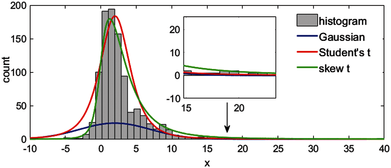
Figure 1: Skew t distribution has better fitting than symmetric distributions

In this paper, a new skew t cubature Kalman filter (STCKF) is proposed for nonlinear system with heavy-tailed and skewed measurement noise. The skew t distribution is adopted to describe the measurement noise and the prior distributions of the shape matrix, scale matrix and DOF are chosen as Gaussian, inverse Wishart and Gamma distributions, respectively. The unknown statistics including shape matrix, scale matrix and DOF are inferred with the VB approach and the posterior of states is also simultaneously obtained. The results of simulation demonstrate that the proposed STCKF has better estimation accuracy as compared with the CKF and Student’s t distribution-based CKF.

The paper is structured as follows: Section 2 describes the problem studied in this paper. Section 3 proposes a skew t cubature Kalman filter based on VB inference. In Section 4, an example of target tracking is presented to verify the estimation performance of the proposed STCKF. The conclusions of this paper are given in Section 5.

Notations: RK denotes the K-dimensional Euclidean space, E[⋅] and tr(⋅) represent the expectation operator and the trace operator, I is the identity matrix with appropriate dimension, AT is the transpose of matrix A, diag(⋅) is the diagonal matrix, N(x,P) is a Gaussian distribution with mean vector x and covariance matrix P, N+(μ,Σ) represents the truncated Gaussian distribution in positive orthant, and its location is μ and scale matrix is Σ.

2  Problem Formulation

Consider the nonlinear state-space model

xn=f(xn−1)+wn−1, (1)

zn=h(xn)+vn, (2)

where n is the discrete time index, f(⋅) and h(⋅) are the nonlinear state function and measurement function, zn∈Rd is the measurement vector, xn∈Rm is the state vector. The process noise wn is Gaussian white noise and wn∼N(0,Qn). The measurement noise vn is the heavy-tailed and asymmetric noise. The initial state vector x0 is assumed to have a Gaussian distribution,

p(x0)=N(x0;x0|0,P0|0). (3)

The skew t distribution is used to describe the heavy-tailed and asymmetric of noise, therefore, the measurement noise vn:

p(vn)=ST(vn;0,Δn,Rn,νn). (4)

where ST(vn;0,Δn,Rn,νn) denotes the skew t distribution with location 0, shape matrix Δn, scale matrix Rn and DOF νn. Specifically, the definition of skew t distribution can be seen in [30,32].

Fig. 2 shows the different Δ of distributions ST(x;0,1,Δ,3). As shown, with the decreasing of Δ, the skew t distribution will deteriorate to the Student’s t distribution. Therefore, the skew t distribution has both heavy-tails and asymmetric properties with suitable values.

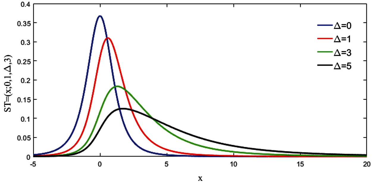
Figure 2: Different Δ for ST(x;0,1,Δ,3)

In the following, based on the CKF, we will design a nonlinear filter under nonlinear model (1)–(2) with the measurement noise followed by skew t distribution. Specifically, the statistics of skew t distribution including the shape matrix, the scale matrix and the DOF are unknown and need to be estimated together with the system states by using VB inference.

3  Proposed Skew t Cubature Kalman Filter Using VB Inference

3.1 Prior Distributions Update

Similar to CKF, the predicted distribution of system state xn is

p(xn|z1:n−1)=N(xn;xn|n−1,Pn|n−1), (5)

where xn∣n−1 and Pn|n −1 can be approximated by the CKF here. More specifically, the cubature points are obtained by

χ¯i,n−1=xn−1|n−1+Pn−1|n−1ξi, (6)

where i=1,⋯,2m, ξi=m×[1]i, and [1]i denotes the i-th element of the following set:

The predicted cubature points are

χi,n−1=f(χ¯i,n−1), (7)

Hence, the predicted state and the corresponding error covariance are given by

xn|n−1=12m∑i=12mχi,n−1 (8)

Pn|n−1=12m∑i=12mχi,n−1χi,n−1T−xn|n−1xn|n−1T+Qn−1. (9)

In Bayesian theory, the conjugate prior needs ensure posterior distribution have the same functional form with prior distribution. Therefore, to infer shape matrix Δn, scale matrix Rn, and DOF νn, the conjugate priors of Δn, Rn, and νn need to be selected. The prior distribution of Δn is selected as Gaussian distribution [33]:

p(Δn|z1:n−1)=∏j=1dN(Δn,j;μn|n−1,j,σn|n−1,j), (10)

where μn|n−1,j is the predicted mean of j-th dimension and σn|n−1,j is the corresponding variance, respectively. The prior distribution of Rn is selected as inverse Wishart distribution [21]:

p(Rn|y1:n−1)=IW(Rn;cn|n−1,Dn|n−1), (11)

where Dn|n −1 and cn|n −1 are the inverse scale matrix and DOF, respectively. The prior distribution of νn is selected as Gamma distribution [26]:

p(νn|z1:n−1)=G(νn;an|n−1,bn|n−1), (12)

where an|n −1 and bn|n −1 are the shape parameter and the rate parameter, respectively.

To obtain (10)–(12), the dynamic model p(Δn|Δn−1), p(Rn|Rn −1) and p(νn|νn−1) need to be specified. In practice, the variation of the measurement noise parameters is slow, and we can use a forgetting factor ρ∈(01] to describe the predicted distribution in this paper [21]:

μn|n−1,j=ρμn−1|n−1,j,σn|n−1,j=ρσn−1|n−1,j, (13)

cn|n−1=ρ(cn−1|n−1−d−1)+d+1,Dn|n−1=ρDn−1|n−1, (14)

an|n−1=ρan−1|n−1,          bn|n−1=ρbn−1|n−1. (15)

Because of the skewed t distribution does not have a strictly closed form, the state posterior distribution will be difficult to obtain. With the introduction of two hidden variables un and Λn, the likelihood p(zn|xn) can be rewritten by the following hierarchical Gaussian model [30]:

p(zn|xn,Δn,un,Λn,Rn)=N(h(xn)+Δnun,Λn−1Rn), (16)

p(un|Λn)=N+(0,Λn−1), (17)

p(Λn|νn)=G(νn2,νn2). (18)

3.2 Posterior Estimation

In order to estimate xn from (5), (10)–(12), and (16)–(18), the joint posterior (pxn,Δn,un, Λn,Rn,νn|z1:n) needs to be computed. According to Bayes’ theorem,

p(H|z1:n)=p(zn|H)p(H|z1:n−1)p(zn|z1:n−1), (19)

where H={xn,Δn,un,Λn,Rn,νn}. Due to inter-coupled parameters, it is infeasible to infer the posterior p(H|z1:n) analytically. From (19), the logarithmic marginal likelihood log⁡p(zn|z1:n−1) can be derived as [35]

log⁡p(zn|z1:n−1)=KLD(q(H)‖p(H|z1:n))+L(q(H)), (20)

where KLD(⋅) and L are the Kullback-Liebler divergence and the lower bound of log⁡p(zn|z1:n−1), respectively. Due to the non-negativity of the KLD, we can obtain the true posterior by minimizing the KLD between q(H) and p(H|z1:n) [35,36]. Thus, the fix-point iteration of VB inference is utilized to approximate p(xn,Δn,un,Λn,Rn,νn|z1:n) by means of the product of some individual distributions [21,37], i.e.,

p(xn,Δn,un,Λn,Rn,νn|z1:n)≈q(xn)q(Δn)q(un)q(Λn)q(Rn)q(νn), (21)

where q(⋅) represents the approximate posterior of p(⋅). An analytical solution of q(xn), q(Δn), q(un), q(Λn), q(Rn), and q(νn) can be obtained by [21]

log⁡q(φ)=EH(−φ)[log⁡p(zn,H|z1:n−1)]+cφ (22)

where φ is an element of H, H(−φ) is all elements in H except for φ, and cφ is the constant on the variable φ.

Based on Bayesian theory, we can obtain the joint posterior distribution as follows:

p(zn,H|z1:n−1)=p(zn|H)p(H|z1:n−1)=p(zn|xn,Δn,un,Λn,Rn)p(xn|z1:n−1)p(Δn|z1:n−1)p(un|Λn)p(Λn|νn)×p(Rn|cn|n−1,Dn|n−1)p(νn|an|n−1,bn|n−1). (23)

Substituting (5), (10)–(12), and (16)–(18) into (23) results in

p(zn,H|z1:n−1)=N(zn;h(xn)+Δnun,Λn−1Rn)N(xn;xn|n−1,Pn|n−1)∏j=1dN(Δn,j;μn|n−1,j,σn|n−1,j)×N+(un;0,Λn−1)G(Λn;νn2,νn2)IW(Rn;cn|n−1,Dn|n−1)G(νn;an|n−1,bn|n−1). (24)

When φ=xn, the posterior distribution q(xn) is calculated as:

q(xn)=N(xn;xn|n,Pn|n), (25)

where xn|n and Pn|n are the estimate of state and the corresponding covariance respectively, and can be obtained by

χi,n|n−1=xn|n−1+Pn|n−1ξi, (26)

z¯n=12m∑i=12mh(χi,n|n−1), (27)

Pxz,n=12m∑i=12m(χi,n|n−1−xn|n−1)(h(χi,n|n−1)−z¯n)T, (28)

Pzz,n=12m∑i=12m(h(χi,n∣n−1)−z¯n)(h(χi,n∣n−1)−z¯n)T+R~n, (29)

Kx=Pxz,nPzz,n−1, (30)

xn|n=xn|n−1+Kx(zn−z¯n−E[Δn]E[un]), (31)

Pn|n=Pn|n−1−KxPzz,nKx, (32)

where R~n={E[Rn−1]}−1E[Λn]. The derivation of (25)–(32) can be seen in Appendix A.

When φ=Δn, the posterior distribution q(Δn) is calculated as

q(Δn)=∏j=1dN(Δn,j;μn|n,j,σn|n,j), (33)

where the mean μn|n,j and variance σn|n,j are given by

KΔ,j=σn|n−1,jE[un,j](σn|n−1,j(E[un,j])2+R~n,j)−1, (34)

μn|n−1,j+KΔ,j(εn,j−E[un,j]μn|n−1,j), (35)

σn|n,j=σn|n−1,j−σn|n−1,jE[un,j]KΔ,j, (36)

where εn=E[zn−h(xn)]. The derivation of (33)–(36) can be seen in Appendix B.

When φ=un, the posterior distribution q(un) is calculated as

q(un)=N+(un;un|n,Un|n), (37)

where the location un|n and covariance Un|n are obtained by

Ku=E[Δn]((E[Δn])2+R~n)−1, (38)

un|n=Kuεn, (39)

Un|n=(I−KuE[Δn])(E[Λn])−1. (40)

The derivation of (36)–(40) can be seen in Appendix B.

When φ=Λn, the posterior distribution q(Λn) is calculated as

q(Λn)=G(Λn;αn,βn), (41)

where the shape parameter αn and the rate parameter βn are given by

αn=12(E[νn]+m), (42)

βn=12(Ψn+E[νn]), (43)

where ψn is an auxiliary parameter and the derivation of (41)–(43) can be seen in Appendix C.

When φ=Rn, the posterior distribution q(Rn) is calculated as

q(Rn)=IW(Rn;cn∣n,Dn∣n), (44)

where the DOF cn|n and inverse scale matrix Dn|n are obtained by

cn|n=cn|n−1+1, (45)

Dn|n=ϒn+Dn|n−1, (46)

where Υn is an auxiliary parameter and the derivation of (44)–(46) can be seen in Appendix C.

When φ=νn, the posterior distribution q(νn) is calculated as

q(νn)=G(νn;an∣n,bn∣n), (47)

where the parameters an and bn are given by

an∣n=an∣n−1+12, (48)

bn|n=bn|n−1−12−12E[logΛn]+12E[Λn]. (49)

The derivation of (47)–(49) can be seen in Appendix D.

Using (25), (33), (36), (41), (44), and (47), the following expectations are required:

E[Λn]=αn/βn, (50)

E[Rn−1]=(cn∣n−M−1)Dn∣n−1, (51)

E[νn]=an∣n/bn∣n, (52)

E[Δn]=diag(μn∣n,1,⋯,μn∣n,d), (53)

E[logΛn]=ψ(αn)−logβn, (54)

where ψ(⋅) denotes the digamma function. The computations of E[un] and E[ununT] can be found in [38].

After taking N fix-point iteration steps, the approximations of posterior distributions are updated as

q(xn)≈N(xn;xn∣n(N),Pn∣n(N))=N(xn;xn∣n,Pn∣n), (55)

q(Δn)≈∏j=1dN(Δn,j;μn∣n,j(N),σn∣n,j(N))=∏j=1dN(Δn,j;μn∣n,j,σn∣n,j), (56)

q(un)≈N+(un;un∣n(N),Un∣n(N))=N+(xn;un∣n,Un∣n), (57)

q(Λn)≈G(Λn;αn(N),βn(N))=G(Λn;αn,βn), (58)

q(Rn)≈IW(Rn;cn∣n(N),Dn∣n(N))=IW(Rn;cn∣n,Dn∣n), (59)

q(νn)≈G(νn;an|n(ℕ),bn|n(ℕ))=G(νn;an|n,bn|n). (60)

Combining prediction steps (5) and (10)–(12) with measurement updates (25), (33), (36), (41), (44) and (47), the proposed STCKF can be realized recursively. To implement the proposed filter, the initial shape matrix Δ0, the initial scale matrix R0, the initial DOF ν0, and the forgetting factor ρ need to be determined. Generally, Δ0, R0, and ν0 can be approximately achieved from prior knowledge. The forgetting factor ρ can determine how much information from the previous estimation. That is, choosing a small ρ means forgetting more information and vice versa. In the proposed STCKF, the selection of N is a trade-off. Increasing N will obtain better estimation accuracy but more time-consuming.

4  Target Tracking Simulation

To validate the estimation performance of the proposed STCKF, a target tracking simulation is introduced to perform an evaluation of the results obtained. The STCKF is compared with the CKF [16], the Student’s t distribution based-CKF (T-CKF) [25], and the robust Student’s t distribution-based CKF (RT-CKF) [26].

In this paper, a typical air traffic control scenario is considered, in which the aircraft performs maneuvering turns on the horizontal plane at a constant but unknown turning rate Ω. The kinematics of rotational motion can be described by the following nonlinear state-space model [16]:

xn=[ 1sinΩTΩ0−(1−cosΩTΩ)00cosΩT0−sinΩT00(1−cosΩTΩ)1sinΩTΩ00sinΩT0cosΩT000001 ]xn−1+wn, (61)

zn=[ ξn2+ηn2arctanηnξn ]+vn, (62)

where the state x=(ξξ˙ηη˙Ω)T, the position and velocity of target in x and y directions are (ξ,η) and (ξ˙,η˙), T is the time interval and Ω is the tuning rate. The process noise covariance is Qn=diag (q1M, q1M, q2T), where

The associated parameters are set as: q1=0.1 m2s−3, q2=1.75×10−4 s−3, Ω=−3∘ s−1, T=1 s. The true initial state and the corresponding covariance are x0=(1000,300,1000,0,−3)T and P0 =diag (100, 10, 100, 10, 100), respectively.

In this simulation, we consider three cases for measurement noise:

Case 1: Gaussian distribution, that is, vn∼N(0,Rn) with noise covariance Rn=diag(100,10),

Case 2: Contaminated Gaussian distribution (mixture Gaussian distribution). The mixture Gaussian distributed noise is generated according to [33]

vn∼{N(0,Rn)w.p.1−pcN(0,100Rn)w.p.pc, (63)

where Rn=diag(100,10). Eq. (63) means that vn is drawn from N(0,Rn) with probability 1 − pc and N(0,100Rn) with probability pc. In this paper, pc = 0.1.

Case 3: Contaminated skew t distribution (mixture skew t distribution).

According to [32], the measurement noise vn is generated by

vn∼{ST(0,Rn,Δn,νn)w.p.1−pcST(0,10Rn,Δn,νn)w.p.pc, (64)

where Rn=diag(100,10), Δn=diag(5,5), and νn=4.

In this paper, the root mean square error (RMSE) is adopted to test the filtering performance, and its formula is

RMSEn=1M∑j=1M‖xn∣nj−xnj‖2, (65)

where xn∣nj and xnj are the estimated and true values, respectively, at the j-th Monte-Carlo run. The simulated inputs are a0 = 4, b0 = 1, c0 = 3, D0=diag(1,1), μ0=diag(1,1), σ0=diag(1,1) , ρ=1−exp⁡(−5) and N=5.

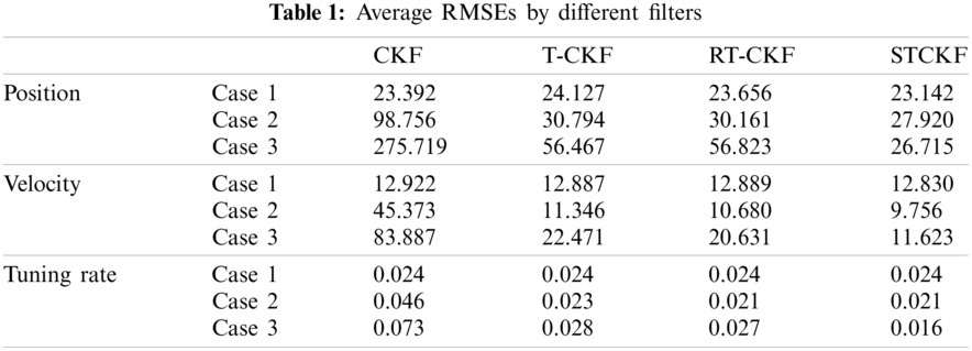
Figs. 3–5 show that the RMSEs of position, velocity, and tuning rate based on 20 Monte-Carlo runs for three cases. From Fig. 3, the CKF, T-CKF, RT-CKF and the proposed STCKF almost have the same estimation accuracy under Gaussian distribution noise. However, the methods based on the non-Gaussian distribution outperform the methods based on the Gaussian distribution when the measurement noise no longer satisfies the Gaussian distribution. As shown in Fig. 4, the non-Gaussian filters (T-CKF, RT-CKF and STCKF) perform better than the CKF. From Fig. 5, the proposed STCKF obtains the best accuracy in the case of asymmetric noise distribution and unknown noise statistics. As also observed in Table 1, the filter based on the skewed t distribution and the filters based on the Student’s t distribution perform better than the filter based on the Gaussian distribution in Cases 2 and 3, and the proposed STCKF is significantly better than other filters for the asymmetric noise distribution.

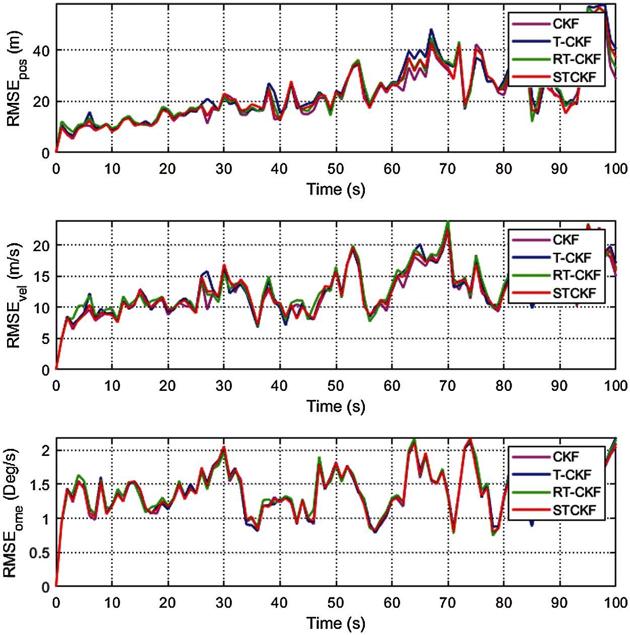
Figure 3: RMSEs of the position, velocity, and tuning rate by different filters under Case 1

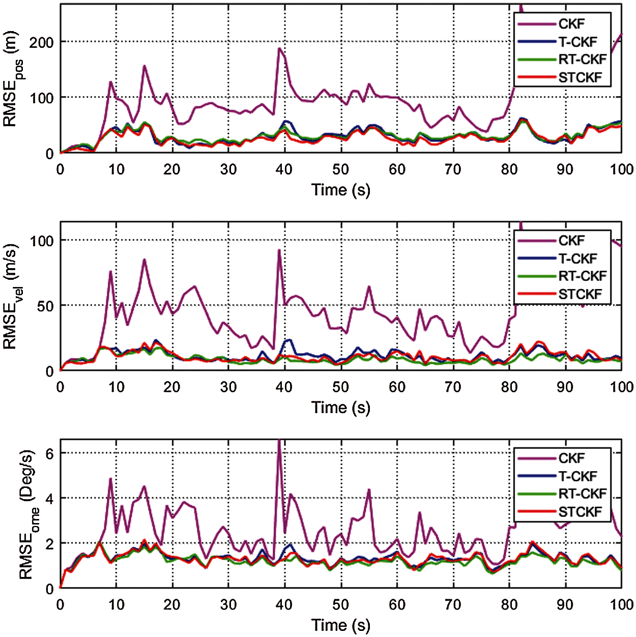
Figure 4: RMSEs of the position, velocity, and tuning rate by different filters under Case 2

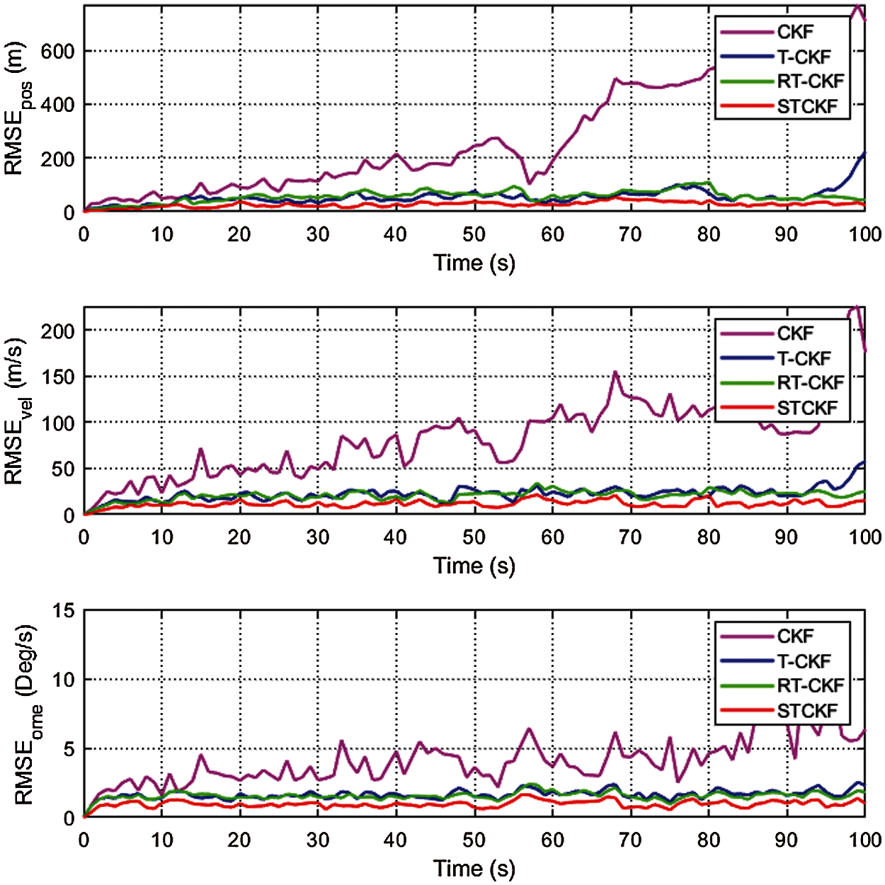
Figure 5: RMSEs of the position, velocity, and tuning rate by different filters under Case 3

5  Conclusion

In this work, we consider the joint estimation problem of system states and unknown noise statistics for nonlinear discrete-time systems. Combining with the properties of skew t distribution, a hierarchical nonlinear Gaussian model is developed. Based on this model, a skew t cubature Kalman filter is proposed, in which the states, shape matrix, scale matrix and DOF are simultaneously estimated by using VB approach. The results of simulation show that the proposed filter in this paper has better estimation accuracy than the conventional CKF and the Student’s t distribution-based CKF under heavy-tailed and skewed measurement noise. It should be noted that the proposed method in this paper can only realize state estimation of asymmetric measurement noise. How to extend the proposed method to handle asymmetric process and measurement noise is still an open problem.

Funding Statement: This work was supported in part by National Natural Science Foundation of China under Grants 62103167 and 61833007, and in part by the Natural Science Foundation of Jiangsu Province under Grant BK20210451.

Conflicts of Interest: The authors declare that they have no conflicts of interest to report regarding the present study.

Appendix A

Substituting φ=xn into (22) yields

log⁡q(xn)=−12(zn−h(xn)−E[Δn]E[un])TE[Rn−1]E[Λn](zn−h(xn)−E[Δn]E[un])−12(xn−xn∣n−1)TPn∣n−1−1×(xn−xn∣n−1)+cx. (66)

Defining the modified likelihood distribution p(zn|xn) as

p(zn|xn)=N(h(xn)+E[Δn]E[un],R~n), (67)

and using (5) and (67) in (66), we have

q(xn)∝N(zn;h(xn)+E[Δn]E[un],R~n)N(xn;xn∣n−1,Pn∣n−1). (68)

According to (5) and (66)–(68), (25)–(32) can be obtained.

Appendix B

Substituting φ=Δn into (22) yields

log⁡q(Δn)=−12(εn−ΔnE[un])TE[Rn−1]E[Λn](εn−ΔnE[un])−∑j=1d12(Δn,j−μn∣n−1,j)Tσn∣n−1,j−1(Δn,j−μn∣n−1,j)+cΔ, (69)

where the auxiliary parameter εn is given by

εn=E[zn−h(xn)]=zn−h(xn∣n). (70)

Substituting φ=un into (22), we have

log⁡q(un)=−12(εn−E[Δn]un)TE[Rn−1]E[Λn](εn−E[Δn]un)−12(unTE[Λn]un)+cu. (71)

Similar to (66)–(68), (33)–(40) can be obtained.

Appendix C

Substituting φ=Λn into (22), we have

log⁡q(Λn)=−12ΛnΨn+(⟨νn⟩+d2−1)log⁡Λn−⟨νn⟩2Λn+cΛ, (72)

where

Ψn=tr(E[Rn−1]E[(zn−h(xn))(zn−h(xn))T]−tr(E[Rn−1]E[Δn]E[un]εnT)−tr(E[Δn]E[Rn−1]εnE[un]T)+tr((E[Δn]E[Rn−1]E[Δn]+I)E[ununT]). (73)

Substituting φ=Rn into (22) yields

log⁡q(Rn)=−12(cn∣n−1+d+2)log⁡|Rn|−12tr((Υn+Dn∣n−1)Rn−1)+cR. (74)

where

Υn=E[Λn]E[(zn−h(xn))(zn−h(xn))T]+E[Λn]E[ΔnΔnT]E[ununT]−E[Λn]E[Δn]E[un]εnT−E[Λn]E[Δn]εnE[un]T. (75)

According to (72) and (74), (41)–(46) can be obtained.

Appendix D

Substituting φ=νn into (22) yields

log⁡q(νn)=νn2log⁡νn2−log⁡Γ(νn2)+(νn2−1)E[log⁡Λn]−νn2E[Λn]+(an∣n−1−1)log⁡νn−bn∣n−1νn+cν. (76)

Using Stirling’s approximation: log⁡Γ(νn2)≈νn−12log⁡(νn2)−νn2 [26], log⁡q(νn) can be rewritten as

logq(νn)=(an∣n−1+12−1)log⁡νn−(bn∣n−1−12−12E[log⁡Λn]+12E[Λn])νn+cν. (77)

According to (77), (41)–(43) can be obtained.

This work is licensed under a Creative Commons Attribution 4.0 International License, which permits unrestricted use, distribution, and reproduction in any medium, provided the original work is properly cited.