Computer Modeling in Engineering & Sciences

DOI: 10.32604/cmes.2022.018778

ARTICLE

On Degenerate Array Type Polynomials

Lan Wu1, Xue-Yan Chen1, Muhammet Cihat Dağli2 and Feng Qi3,4,*

1Key Laboratory of Intelligent Manufacturing Technology, Inner Mongolia Minzu University, Tongliao, 028000, Inner Mongolia, China
2Department of Mathematics, Akdeniz University, Antalya, 07058, Turkey
3Institute of Mathematics, Henan Polytechnic University, Jiaozuo, 454010, China
4School of Mathematical Sciences, Tiangong University, Tianjin, 300387, China
*Corresponding Author: Feng Qi. Email: qifeng618@gmail.com
Dedicated to retired Professor Ji-Shan Tian, former vice president of Henan University, China
Received: 17 August 2021; Accepted: 27 October 2021

1  Introduction

In this paper, we use the following notation:

The Stirling numbers of the second kind S(n, m) for n≥m≥0 can be generated by

(et−1)mm!=∑n=m∞S(n,m)tnn! (1)

and can be computed as

See [[1], p.206] and the paper [2].

The λ-array type polynomials S(n,m;x;λ) were defined in [3] by the generating function

(λet−1)mm!ext=∑n=0∞S(n,m;x;λ)tnn!. (2)

See also the papers [4,5]. It is clear that S(n, m;0;1) = S(n, m). In the paper [6], Simsek obtained and constructed several generating functions and many relations of generalized Stirling type numbers, the array type polynomials, and Eulerian type polynomials. In the paper [7], Bayad et al. deduced interesting and meaningful identities associated with λ-array type polynomials, λ-Stirling numbers of the second kind, and the Apostol–Bernoulli numbers, while they dealt with λ-array polynomials by applying λ-delta operator. Readers interested to the Apostol-Bernoulli numbers and polynomials may consult to the papers [8–10] and closely related references therein.

In the paper [11], Carlitz introduced degenerate Bernoulli and Euler polynomials Bn(x;γ) and En(x;γ) by

t(1+γt)1/γ−1(1+γt)x/γ=∑n=0∞Bn(x;γ)tnn! (3)

and

2(1+γt)1/γ+1(1+γt)x/γ=∑n=0∞En(x;γ)tnn! (4)

respectively. For x = 0, the quantities Bn(0;γ) and En(0;γ) are called as degenerate Bernoulli and Euler numbers. Since limγ→0(1+γt)1/γ=et, Eqs. (3) and (4) reduce to the generating functions for classical Bernoulli and Euler polynomials, respectively.

We now define degenerate λ-array type polynomials S(n,m;x;λ;γ) by

[λ(1+γt)1/γ−1]mm!(1+γt)x/γ=∑n=0∞S(n,m;x;λ;γ)tnn!. (5)

It is easy to see that

limγ→0S(n,m;x;λ;γ)=S(n,m;x;λ) (6)

which is defined by (2). When x = 0, we call the quantities S(n,m;0;λ;γ) degenerate λ-array type numbers.

In this paper, utilizing the Faá di Bruno formula and an identity of the Bell polynomials of the second kind, we establish several explicit formulas and recurrence relations of (degenerate) λ-array type numbers and polynomials.

Let us notice that the Faá di Bruno formula, which can be viewed as an extension of chain rule to higher derivatives, has been applied to establish explicit and closed-form formulas of many important numbers and polynomials in analytic and combinatorial number theory. For more details, please refer to, for example, the papers [12–18] and closely related references therein.

2  Some Identities of the Bell Polynomials of the Second Kind

The Bell polynomials of the second kind Bn,k(x1,x2,…,xn−k+1) for n≥k≥0 can be defined by

See [[1], p. 134]. For n∈N, the Faà di Bruno formula is described in [[1], p.139] in terms of the Bell polynomials of the second kind Bn,k(x1,x2,…,xn−k+1) by

dndtnf∘h(t)=∑k=1nf(k)(h(t))Bn,k(h′(t),h″(t),…,h(n−k+1)(t)). (7)

The formula

Bn,k(1,1−λ,(1−λ)(1−2λ),…,∏ℓ=0n−k(1−ℓλ))=(−1)kk!∑ℓ=0k(−1)ℓ(kℓ)∏q=0n−1(ℓ−qλ) (8)

has been applied and reviewed in [[16], Lemma 2.2], [[17], Remark 6.1], and [[19], Section 1.3]. The explicit formula (8) is equivalent to

Bn,k(⟨λ⟩1,⟨λ⟩2,…,⟨λ⟩n−k+1)=(−1)kk!∑ℓ=0k(−1)ℓ(kℓ)⟨λℓ⟩n, (9)

which was presented in [[20], Theorems 2.1 and 4.1], where the falling factorial ⟨x⟩n is defined for x∈C by

When n∈N, the explicit formulas (8) and (9) can be rearranged as

Bn,k(1,1−λ,(1−λ)(1−2λ),…,∏ℓ=0n−k(1−ℓλ))={(−1)kλnn!k!∑ℓ=0k(−1)ℓ(kℓ)(ℓ/λn),λ≠0;S(n,k),λ=0, (10)

where extended binomial coefficient (zw) is defined by

(zw)={Γ(z+1)Γ(w+1)Γ(z−w+1),z∉N−,w,z−w∉N−0,z∉N−,w∈N− or z−w∈N−⟨z⟩ww!,z∈N−,w∈N0⟨z⟩z−w(z−w)!,z,w∈N−,z−w∈N00,z,w∈N−,z−w∈N−∞,z∈N−,w∉Z (11)

and the classical Euler gamma function Γ(z) can be defined by

For new results and applications about the Bell polynomials‘ of the second kind Bn, k, please refer to the papers [13,19,21–23] and closely related references therein.

3  Explicit Formulas of Degenerate λ-Array Type Polynomials

In this section, we establish two explicit formulas for degenerate λ-array type numbers and polynomials, respectively.

Theorem 3.1. For n∈N, degenerate λ-array type numbers S(n,m;0;λ;γ) can be computed by

S(n,m;0;λ;γ)=n!m!λn(λ−1)m∑k=1n⟨m⟩kk!1(1/λ−1)k∑ℓ=0k(−1)ℓ(kℓ)(ℓ/λn),λ≠0. (12)

Proof. Making use of f(u)=(λu−1)m and u=h(t)=(1+γt)1/γ→1 as t→0 in the Faá di Bruno formula (6) and applying (10) result in

as t→0. Considering the generating function in (5) for x = 0, we proved the explicit formula (12). The proof of Theorem 3.1 is complete.

Remark 3.1. From (5), it follows immediately that

By virtue of the explicit formula (12), we obtain the first few values of degenerate λ-array type numbers S(n,m;0;λ;γ) for 1≤n≤6 as follows:

Remark 3.2. The explicit formula (12) in Theorem 3.1 and seven concrete values listed in Remark 3.1 reveal that degenerate λ-array type numbers S(n,m;0;λ;γ) are polynomials of λ and γ with degrees m and n−1≥0, respectively.

Theorem 3.2. For n∈N, degenerate λ-array type polynomials S(n,m;x;λ;γ) can be computed by

S(n,m;x;λ;γ)=n!m!λn(λ−1)m∑k=1n(−1)kk![∑ℓ=0k(kℓ)⟨m⟩ℓ⟨x⟩k−ℓ(1−1/λ)ℓ][∑ℓ=0k(−1)ℓ(kℓ)(ℓ/λn)]. (13)

Proof. For k∈N, it is easy to see that

as u→1. Letting u=h(t)=(1+γt)1/γ→1 as t→0 and making use of the Faà di Bruno formula (7) give

as t→0. Considering the generating function in (5), we proved the explicit formula (13). The proof of Theorem 3.2 is complete.

Remark 3.3. From the generating function (5), we can easily obtain

By virtue of the explicit formula (13), we can calculate the first few values of degenerate λ-array type polynomials S(n,m;x;λ;γ) for 1≤n≤3 as follows:

Remark 3.4. From the explicit formula (13) in Theorem 3.2 and the four concrete values in Remark 3.3, we conclude that degenerate λ-array type polynomials S(n,m;x;λ;γ) are polynomials of x, λ, and γ of degrees n, m, and n−1≥0, respectively.

Remark 3.5. When x = 0 in Theorem 3.2, the explicit formula (13) becomes (12) in Theorem 3.1.

Remark 3.6. For further better understanding degenerate λ-array type polynomials S(n,m;x;λ;γ), we demonstrate two angles of the graph of S(3,2;4;λ;γ) for −9<λ<9 and 0<γ<9 in Fig. 1. The blue plane in Fig. 1 is the (λ,γ)-plane.

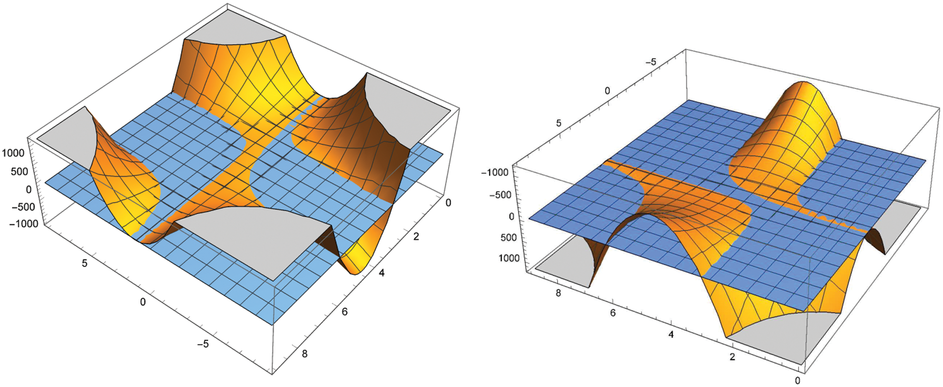
Figure 1: Two angles of the graph of S(3,2;4;λ;γ) for −9<λ<9 and 0<γ<9, plotted by Wolfram Mathematica 12.0

Remark 3.7. For further better understanding degenerate λ-array type polynomials S(n,m;x;λ;γ), we demonstrate two angles of the graph of S(3,2;x;4;γ) for 0 < x < 9 and 0<γ<9 in Fig. 2. The blue plane in Fig. 2 is the (x,γ)-plane.

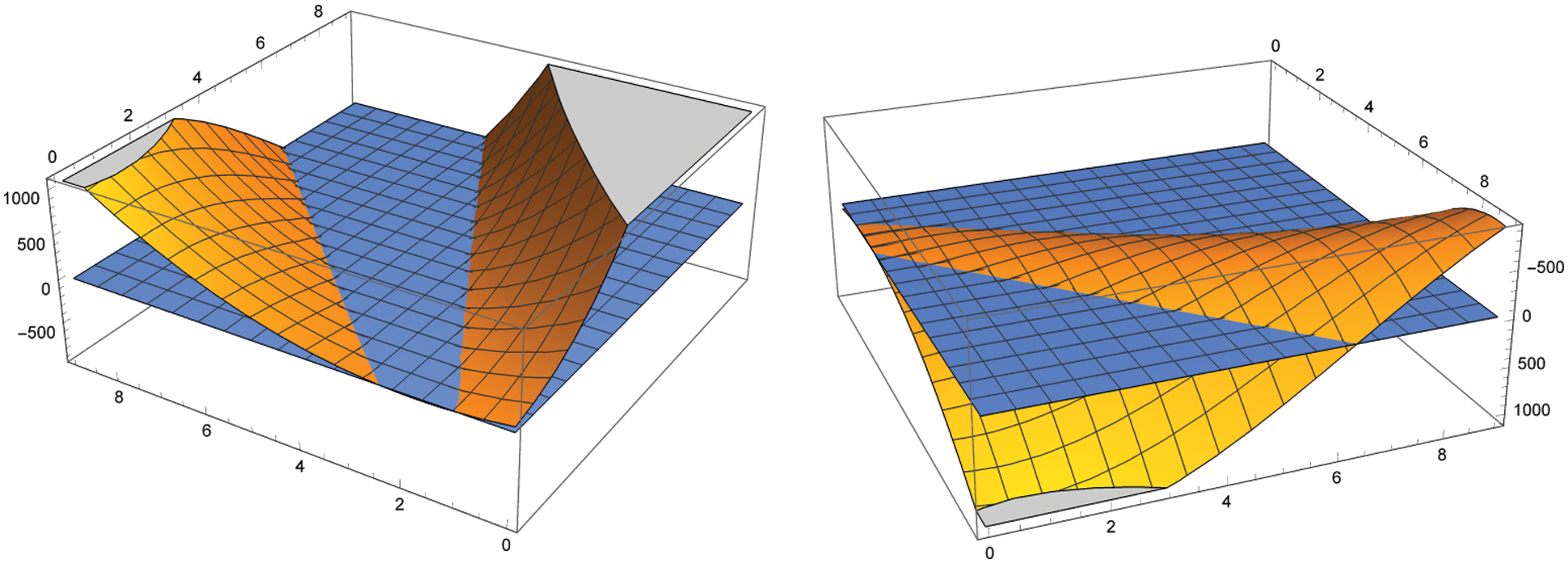
Figure 2: Two angles of the graph of S(3,2;x;4;γ) for 0 < x < 9 and 0<γ<9, plotted by Wolfram Mathematica 12.0

Remark 3.8. For further better understanding degenerate λ-array type polynomials S(n,m;x;λ;γ), we demonstrate two angles of the graph of S(3,2;x;λ;4) for 0 < x < 9 and −9<λ<9 in Fig. 3. The blue plane in Fig. 3 is the (x,λ)-plane.

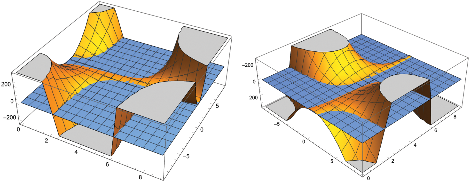
Figure 3: Two angles of the graph of S(3,2;x;λ;4) for 0 < x < 9 and −9<λ<9, plotted by Wolfram Mathematica 12.0

4  Recurrence Relations of Degenerate λ-Array Type Polynomials

In this section, we establish several recurrence relations of degenerate λ-array type polynomials.

Theorem 4.1. Degenerate λ-array type polynomials satisfy the recurrence relation

λS(n,m;x+1;λ;γ)=(m+1)S(n,m+1;x;λ;γ)+S(n,m;x;λ;γ). (14)

Proof. From Eq. (5), it follows that

Comparing coefficients of the terms tnn! on both sides concludes (14). The proof of Theorem 4.1 is complete.

Theorem 4.2. Degenerate λ-array type polynomials S(n,m;x;λ;γ) satisfy the recurrence relation

S(n+1,m;y+γ;λ;γ)=λS(n,m−1;y+1;λ;γ)+(y+γ)S(n,m;y;λ;γ). (15)

Consequently, we have

S(n+1,m;y;λ)=λS(n,m−1;y+1;λ)+yS2(n,m;y;λ). (16)

Proof. Differentiating with respect to t yields

where, on the other hand,

and

Further replacing x by y+γ and simplifying lead to (15).

Taking γ→0 in (15) and considering (6) give (16). The proof of Theorem 4.2 is complete.

Remark 4.1. One of anonymous referees commented that the λ-array type polynomials are related to numbers considered in the papers [24–26].

5  Conclusions

In this paper, with the help of the Faá di Bruno formula (7) and the identity (10) for the Bell polynomials of the second kind Bn, k, we define degenerate λ-array type polynomials S(n,m;x;λ;γ) by (5), establish two explicit formulas (12) and (13) in Theorems 3.1 and 3.2, and present several recurrence relations (14), (15), and (16) of degenerate λ-array type polynomials and numbers S(n,m;x;λ;γ) and S(n,m;λ;γ) in Theorems 4.1 and 4.2.

Acknowledgement: The authors thank the editors and anonymous referees for their careful corrections to, valuable comments on, and helpful suggestions to the original version of this paper.

Funding Statement: The first two authors, Mrs. Lan Wu and Xue-Yan Chen, were partially supported by the College Scientific Research Project of Inner Mongolia (Grant No. NJZY19156 and Grant No. NJZZ19144), by the Natural Science Foundation Project of Inner Mongolia (Grant No. 2021LHMS05030), and by the Development Plan for Young Technological Talents in Colleges and Universities of Inner Mongolia (Grant No. NJYT22051) in China.

Conflicts of Interest: The authors declare that they have no conflicts of interest to report regarding the present study.

This work is licensed under a Creative Commons Attribution 4.0 International License, which permits unrestricted use, distribution, and reproduction in any medium, provided the original work is properly cited.