| Computer Modeling in Engineering & Sciences |
DOI: 10.32604/cmes.2022.019705
ARTICLE
Noise Pollution Reduction through a Novel Optimization Procedure in Passive Control Methods
1Key Laboratory of In-Situ Property-Improving Mining of Ministry of Education, Taiyuan University of Technology, Taiyuan, 030024, China
2Henan International Joint Laboratory of Structural Mechanics and Computational Simulation, Huanghuai University, Zhumadian, 463000, China
3College of Architecture and Civil Engineering, Xinyang Normal University, Xinyang, 464000, China
4The York Management School, University of York, York, YO10 5DD, UK
5CAS Key Laboratory of Mechanical Behavior and Design of Materials, University of Science and Technology of China, Hefei, 230027, China
6Institute for Computational Engineering, Faculty of Science, Technology and Communication, University of Luxembourg, Luxembourg, SA2 8PP, UK
7School of Engineering, Cardiff University, Cardiff, CF24 3AA, UK
8Shanghai Key Laboratory of Digital Manufacture for Thin-Walled Structures, School of Mechanical Engineering, Shanghai Jiao Tong University, Shanghai, 200240, China
*Corresponding Authors: Wenchang Zhao. Email: jsukya@mail.ustc.edu.cn; Mingdong Zhou. Email: mdzhou@sjtu.edu.cn
Received: 10 October 2021; Accepted: 02 November 2021
Abstract: This paper proposes a novel optimization framework in passive control techniques to reduce noise pollution. The geometries of the structures are represented by Catmull-Clark subdivision surfaces, which are able to build gap-free Computer-Aided Design models and meanwhile tackle the extraordinary points that are commonly encountered in geometric modelling. The acoustic fields are simulated using the isogeometric boundary element method, and a density-based topology optimization is conducted to optimize distribution of sound-absorbing materials adhered to structural surfaces. The approach enables one to perform acoustic optimization from Computer-Aided Design models directly without needing meshing and volume parameterization, thereby avoiding the geometric errors and time-consuming preprocessing steps in conventional simulation and optimization methods. The effectiveness of the present method is demonstrated by three dimensional numerical examples.
Keywords: Noise control; topology optimization; Catmull-Clark subdivision surfaces; isogeometric analysis; boundary element methods
Installing sound-absorbing materials on structures is considered as an effective passive control technique to reduce noise level [1–3]. Considering the increase in weight and cost, the full coverage of absorption materials is impractical. Under the volume constraint, the materials should be distributed reasonably to attain a satisfactory soundproofing effect. As a pace-setting technique, topology optimization serves as an effective tool to solve this engineering problem [4–6]. Topology optimization is a mathematical method that optimizes material distribution for particular objective functions and constraints. In topology optimization, the design is improved iteratively until it converges to an optimal solution. The first application of topology optimization in acoustics is traced back to the research of Dhring et al. [6], in which outdoor sound barriers were optimized and remarkable noise reduction was achieved.
As a versatile numerical technique, the finite element method (FEM) is widely used in topology optimization. For acoustic problems, the boundary element method (BEM) is also commonly used for its advantages in dealing with unbounded domain problems [7–12]. However, FEM or BEM relies on a preprocessing step that converts the structural geometries into polygonal meshes, which is time-consuming and results in geometric errors. The isogeometric boundary element method (IGABEM) has recently emerged as a competitive alternative to the conventional numerical methods. The core concept of the IGABEM is to employ basis functions used in Computer-Aided Design (CAD) for geometric modeling to solve boundary integral equation that are transformed from the partial differential equations. As such, IGABEM enables numerical simulation to be conducted from CAD directly which avoids the cumbersome meshing procedure and retains geometric accuracy [13–15]. Unlike isogeometric finite element analysis, a volume parameterization is not needed in IGABEM, because both BEM and CAD are boundary-represented. IGABEM has been successfully applied in linear elasticity [16,17], acoustic analysis [18,19], structural optimization [20 –23], etc.
Subdivision surface modeling is an important CAD technique to represent the complex surface geometries of structures [24–26]. Compared to Non-Uniform Rational B-splines (NURBS), the main merit of subdivision surfaces lies in its ability of constructing gap-free models which are a prerequisite for the numerical analysis. Apart from that, subdivision surfaces are able to tackle extraordinary points at which the curvatures are not bounded. Although many different schemes have been proposed in the category of subdivision surface modeling since its inception [27–30], its first version, the Catmull-Clark subdivision surface [31–33], is still gaining popularity in practice and is being applied to a large variety of engineering problems [34–37]. This may be attributed to its simplicity, generality, and well-established ecosystem. Although the Catmull-Clark subdivision surfaces have been successfully incorporated into IGABEM for numerical simulation [15,38], to the best of our knowledge, no study has been reported on topology optimization thus far.
This study aims to fill this research gap. We propose a topology optimization procedure to design the distribution of sound-absorbing materials, in which the Catmull-Clark subdivision surface is adopted to construct geometric models and its basis functions are used to simulate acoustic fields. The objective is to minimize the noise level subject to the volume constraints of absorption materials. As an extension of our previous work [39] where the Loop subdivision surface was used in IGABEM for topology optimization, the incorporation of Catmull-Clark subdivision surfaces into the acoustic topology optimization procedure enables us to use quadrilateral meshes and thus enhances our capability of geometric modeling. The main strength of the present method arises from its capability of seamlessly integrating numerical analysis and CAD models for complex geometries, which enhances the efficiency and accuracy of topology optimization.
The remainder of this paper is organized as follows. In Section 2, the fundamentals of Catmull-Clark subdivision surface modelling are briefly reviewed for completeness. Section 3 introduces the IGABEM formulation in acoustic analysis that takes into account impedance boundary conditions related to the acoustical effects of absorbing materials. Section 4 formulates the density-based acoustic topology optimization method in which the interpolation scheme of absorption material impedance and the sensitivity analysis with adjoint variable method are highlighted. Section 5 provides numerical examples to verify the correctness and efficiency of the proposed approach, followed by the conclusions in Section 6.
2 Catmull-Clark Subdivision Surfaces
The first step for a designer to build geometries with Catmull-Clark subdivision surfaces is to construct a control grid, which is a polygon mesh with quadrilateral elements whose vertices are called control points. Subsequently, the control grid is subdivided, new control points are introduced, and the positions of the existing control points are updated in Fig. 1. The control grid can be subdivided repeatedly, and the subdivision process from the subdivision level k to the level k + 1 follows the following rule in Fig. 2.
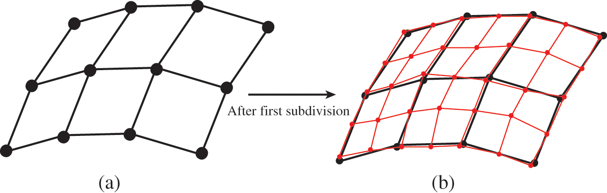
Figure 1: Catmull-Clark subdivision algorithm for surfaces. The black points indicate the control points before the subdivision, and the red points indicate the control points after the subdivision. (a) Initial control mesh (b) One-level refined mesh
• E-vertex: Let the two vertices of the inner edge be
• F-vertex: If the vertices on each face are
• V-vertex: For an internal vertex xk, we denote its one-neighbor vertices by
where

Figure 2: Topology scheme of a Catmull-Clark subdivision surface. The green circle represents the E-vertex inserted at the middle of an edge, the purple circle is the F-vertex inserted at the middle of an element, and the red circle represents the V-vertex formed by the transfer of a vertex in a parent element
After the control points of the subdivided control grid are determined, a smooth surface can be constructed through a linear combination of control points and basis functions:
where ni is the number of basis functions,
where the symbols
Fig. 3 shows an example of a werewolf generated by Catmull-Clark subdivision surfaces. The second row of the figure represents the head, hands, and feet of the werewolf model after it is subdivided once. The example shows that the subdivision surface method is highly adaptable to complex geometry and capable of constructing smooth surfaces. It is noted that the the final smooth geometries are the same regardless of the subdivision times of the control grid.

Figure 3: A werewolf model generated from Catmull-Clark subdivision surfaces. The number of elements in the initial model was 3444, which increases to 13776 after subdivision once
3 Acoustic Simulation Using IGABEM
Numerical simulation using the IGABEM can be used to compute the objective function and evaluate the design performance at each iterative step in the topology optimization process. The acoustic field is governed by the Helmholtz equation in domain
where
where
where
where
The conventional boundary condition may yield fictitious eigen-frequencies. This problem can be resolved by Burton-Miller method [40–45], which is a linear combination of conventional boundary integral equation (Eq. (7)) and its normal derivative. Taking into account the impedance boundary condition, the Burton-Miller method can be formulated as
where
For a structural surface that is modeled using Catmull-Clark subdivision surfaces, whose basis functions Bi are used to discretize the acoustic field around the surface,
where pe and qe denote the acoustic pressure and its normal flux at a field point
To transform the boundary integral equation to linear algebraic equations, we placed the source points at a set of discrete collocation points on the boundary and enforce the governing equations to be satisfied on them. In conventional BEM, the nodes of the mesh are normally chosen as collocation points. In the present work, the collocation points are selected as the points on the smooth surface that are mapped from the nodes of the control grid. With the collocation scheme, the system equation can be rewritten as
where Ne is the number of elements. The above equations can be collected as
where
Because the kernel functions are singular at the source points, the singular integral arises in Eq. (12) which has to be addressed carefully [46,47]. To overcome this problem, the singularity subtraction technique (SST) is adopted in this work. SST subtracts the singular part from the integrand and integrate it analytically. The remaining part of the integrand is regular which can be integrated numerically with Gaussian quadrature.
We consider an optimization problem for the absorbing-material distribution to minimize sound pressures subject to material volume constraints. The topology optimization problem can be formulated as follows:
where the objective function
where matrices
In the present work, the density-based method is used for topology optimization. As a gradient-based optimization algorithm, it is more mathematically sound and converges to the optimized solution more rapidly than the gradient-less optimization methods like genetic algorithms [48]. To tackle a large number of design variables, the adjoint variable method is adopted to compute the sensitivities that play a vital role in density-based topology optimization procedure. In viewing of (13) and (16), we rewrite the objective function by adding zero functions as
where
After rearrangements, Eq. (18) can be reformulated as
where
As mentioned above, the adjoint vectors
Eq. (21) is called adjoint equation. After solving it, the adjoint variables
4.2 Interpolation Scheme of Acoustic Absorbing Materials
According to the Delany-Bazley-Miki model [49], the normalized impedance of sound absorption materials reads
where
To make the material distribution close to a 0–1 design, a material interpolation model, the so-called solid isotropic material with penalization (SIMP) method, is used to interpolate the element admittance:
where
After the sensitivities are evaluated, a gradient-based optimizer can be used to update the design variables until it converges. In the present work, the method of moving asymptotes is used as the optimizer and the convergence criterion is set as
where
A numerical example is presented in this section to investigate the effectiveness of the topology optimization approach using the IGABEM with Catmull-Clark subdivision surfaces. The iterative convergence criterion is set to
Now, we consider the model mentioned in Section 2, which is used to demonstrate the applicability of the proposed optimization method in addressing complex geometries. Herein, the plane wave spreads along the x direction, and the coordinates of the test point used for calculation of objective function are (12, −5, 0). The optimized distribution of sound-absorbing materials at different frequencies is analyzed, and four different frequencies (f = 50, 100, 150 and 200 Hz) are considered in Fig. 4. The color red indicates that the area is covered with sound-absorbing materials, the color blue indicates that the area is rigid. From this figure, we can observe that the final optimized distribution is symmetric with respect to the XOY plane. When the excitation frequency is different, the optimized distribution obtained by calculation is different. This indicates that the optimized distribution of sound-absorbing material has a frequency dependence.
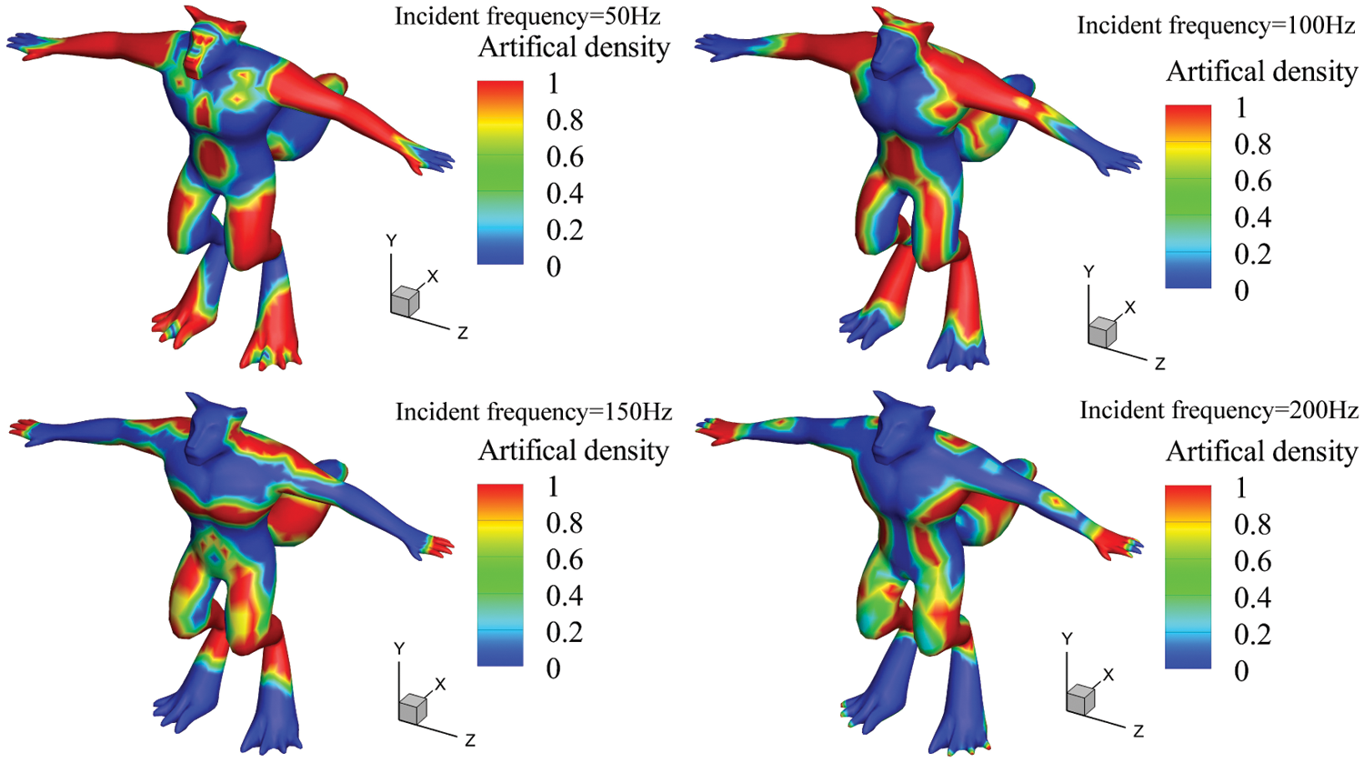
Figure 4: Optimized distribution of sound-absorbing materials of werewolf model at different frequencies
Fig. 5 shows the real part, imaginary part, and amplitude of the sound pressure and its flux on the optimized structural surface at 100 Hz, respectively. A good symmetry along the XOY plane can be observed, and it verifies the correctness of the algorithm developed in this study.
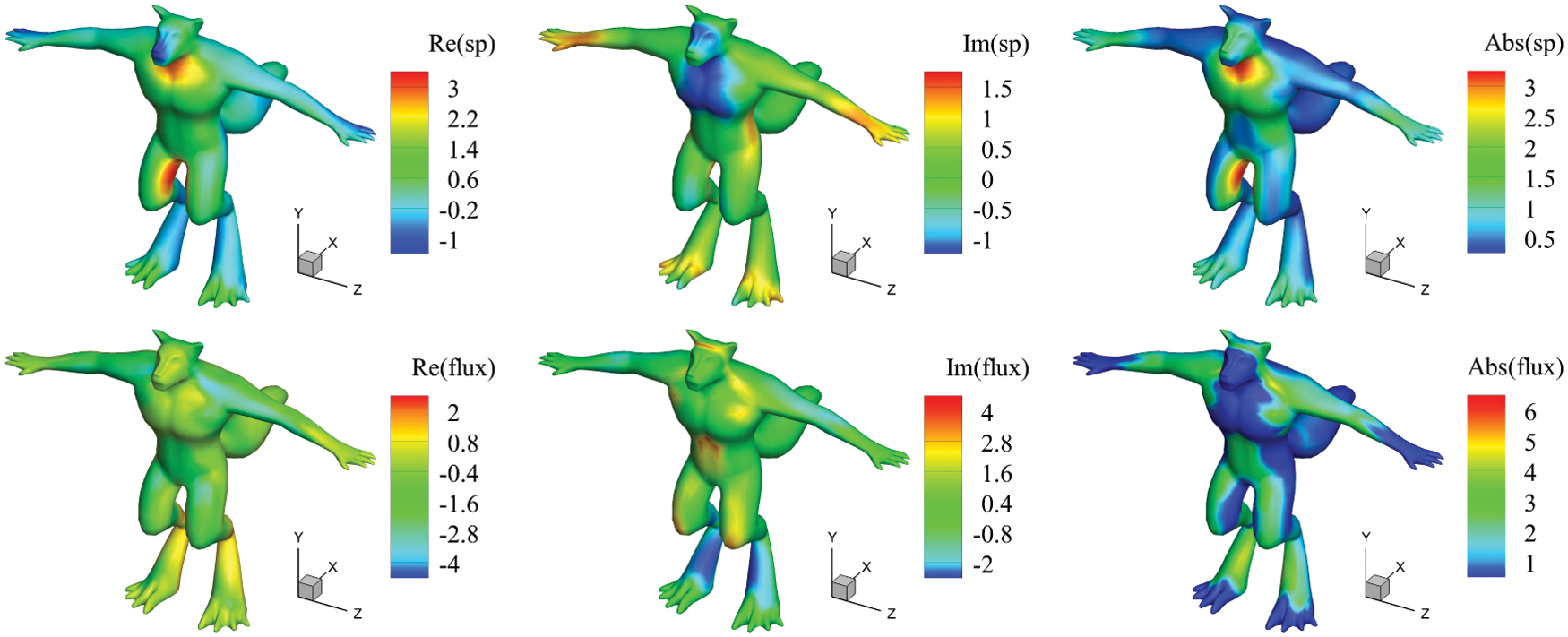
Figure 5: Contour of the acoustic pressure and flux on the werewolf surface with an optimized distribution of sound-absorbing materials
Similarly, when f = 50, 100, 150 and 200 Hz, the distribution of the sound-pressure level after optimization is shown in Fig. 6. We can observe that the higher the frequency, the more intense the change in the distribution of the sound-pressure level. In addition, the value of the sound-pressure level on many structural areas increases with the increase in frequency.
The effect of different parameters on the objective function and material volume constraints is investigated. First, the effect of penalty factor on optimization results is considered. Theoretically, the larger the value of
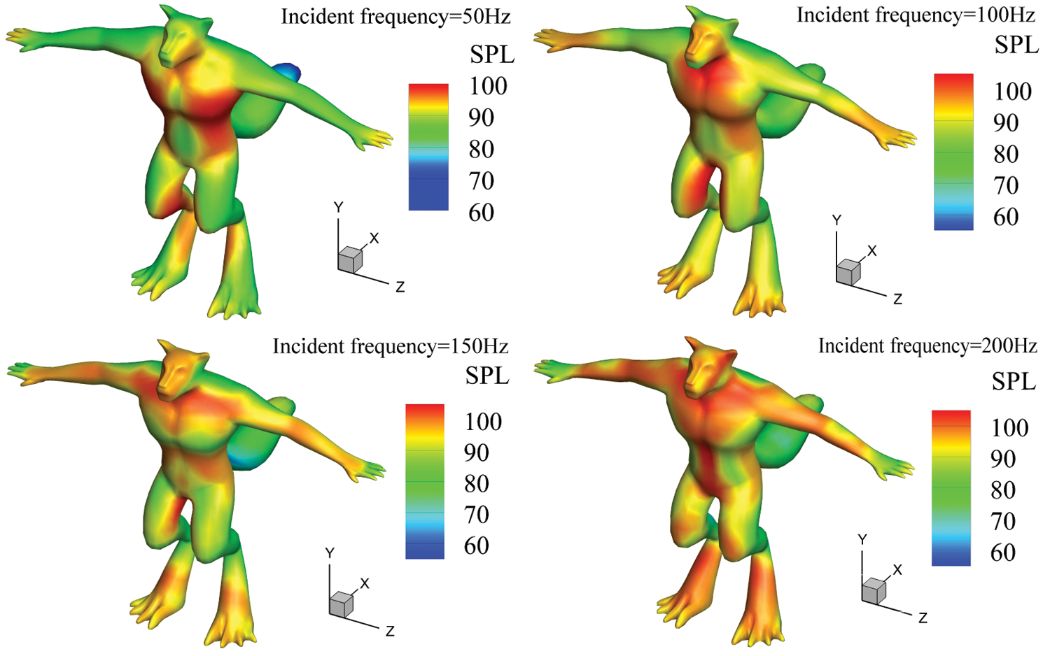
Figure 6: Contour of the acoustic pressure levels (SPL) on the werewolf surface with an optimized distribution of sound-absorbing materials
Figs. 7 and 8 show the objective function and volume fraction function in terms of the iteration step with different values of
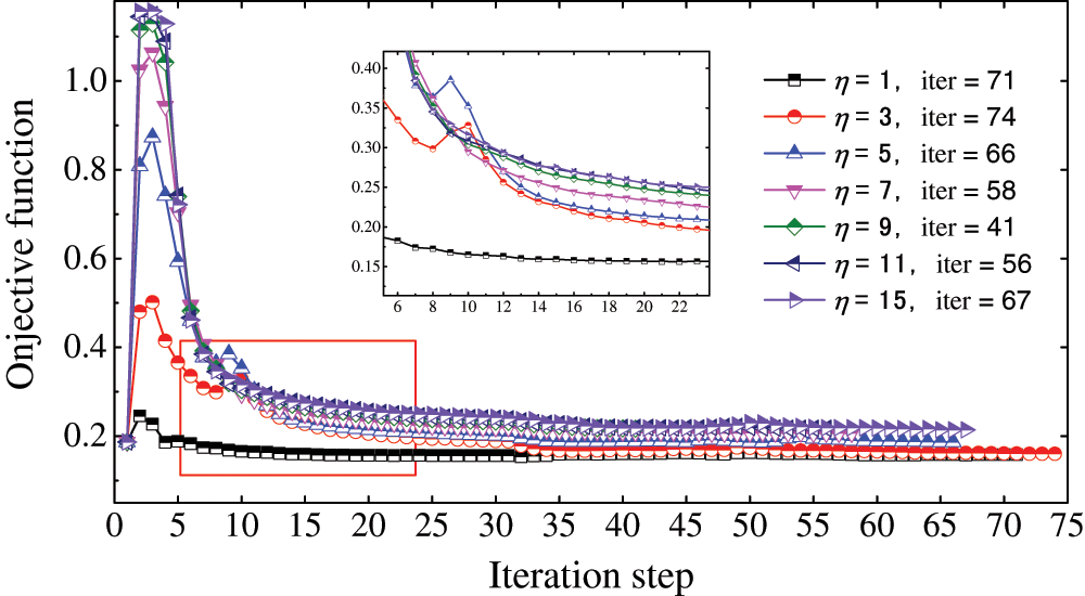
Figure 7: Iteration history of the objective function at different values of
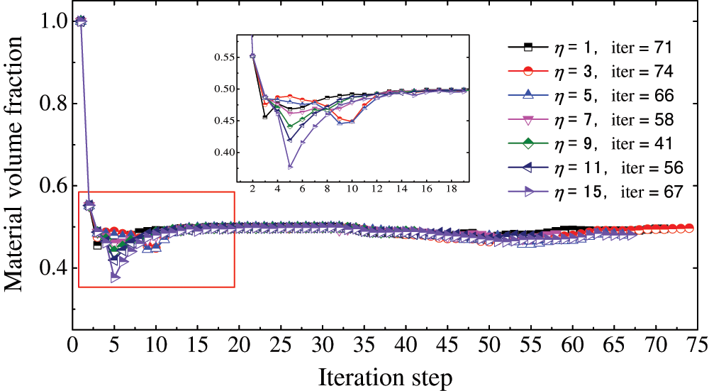
Figure 8: Iteration history of the material volume fraction at different values of
We consider the effects of the initial values of design variables on the optimization results. Figs. 9 and 10 show the objective and material volume fraction functions in terms of iteration steps with different initial values, respectively. The volume constraint is still set as 0.5. We set the initial values as (0.2, 0.4, 0.6, 0.8, 1.0) for comparative analysis. Fig. 9 shows that in the initial iteration step, the initial value of the design variables has a significant effect on the objective function value, but as the iteration steps increase, the effect decreases rapidly until it converges to the same level value. The results indicate that the initial value of design variables has a slight effect on the topology optimization of material distribution.
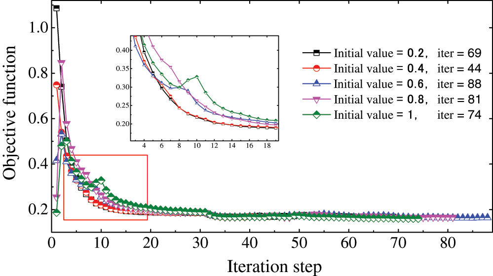
Figure 9: Iteration history of the objective function with different initial values
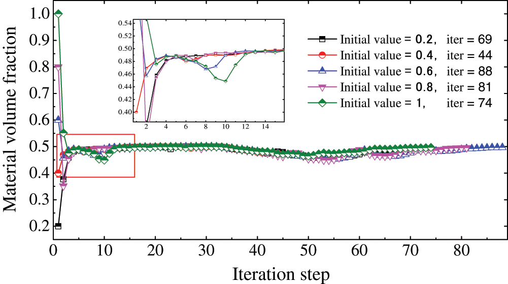
Figure 10: Iteration history of the material volume fraction with different initial values
In this example, a car body shell model is constructed using Catmull-Clark subdivision surfaces with an initial control grid with 2288 elements and 2290 vertices in Fig. 11. We test the proposed algorithm by solving the acoustic scattering problems and optimizing the layout of sound-absorbing materials attached to the car surfaces. The incident plane acoustic wave propagates forward along the x direction, and the excitation frequency is set as 100 Hz. The optimization aim is to minimize the acoustic pressure at a sample Point A with coordinates (20, 5, 0).
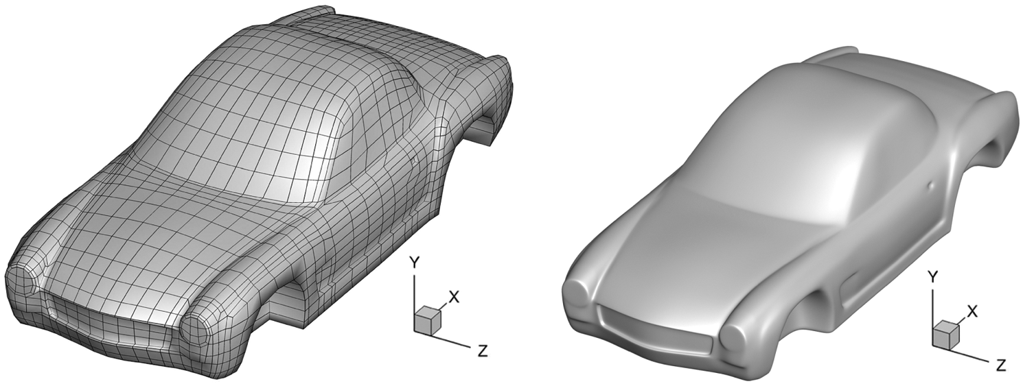
Figure 11: Initial control grid of a car model (left); smooth Catmull-Clark surface of the car model (right)
Herein, the volume ratio constraint is 0.5, that is, at most
In the iteration process of the optimization, the objective and material volume fraction functions vary with the number of iterative steps, as shown in Fig. 12. The objective function initially increases abruptly, decreases rapidly, and finally converges stably because of the full coverage of the initial design. In addition, the material volume ratio decreases rapidly from 1 to 0.35 in the initial several iteration steps, and then remains constant at approximately 0.5 after several steps. Note that although the change in volume ratio is significantly small after the 15-th iteration step, the corresponding material distribution may have an apparent change until convergence is achieved.

Figure 12: Iteration history of the car model after the first subdivision during the optimization process
As the number of iterative steps increases, the optimized distribution of sound-absorbing materials is shown in Fig. 13. We can observe that the optimized distribution is symmetric around the XOY plane, and this is because the original optimization problem is symmetric around the XOY plane. Therefore, for such axisymmetric problems, the symmetric part of the structure can be selected as the optimized object, which can both guarantee the complete symmetry of the final topology design and further reduce the computation. The sound-pressure levels of the car model after the optimization of distribution of sound-absorbing materials is shown in Fig. 14. The acoustic pressure level of the area covered by the acoustic absorbing material is significantly lower than that of the area not covered. Similarly, a noticeable symmetry can be observed. The results verify the correctness of the algorithm and the effectiveness of the optimization analysis of complex models.
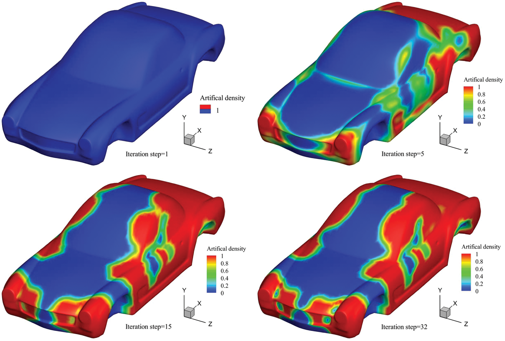
Figure 13: Sound-absorbing material distribution at different iteration steps
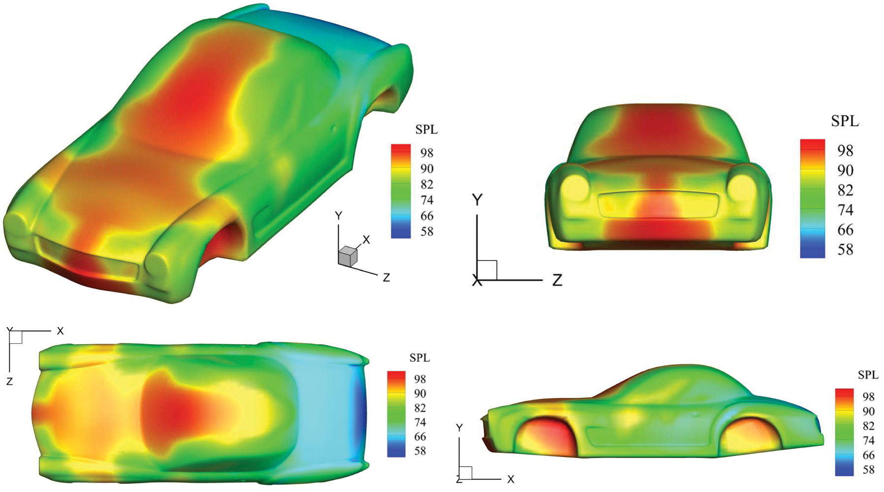
Figure 14: Acoustic pressure (SPL) around the car surface after the distribution of sound-absorbing materials is optimized
In this study, we propose a method to optimize the distribution of sound-absorbing materials in noise pass control techniques based on isogeometric boundary element methods. The complex geometries of components or structures are modeled using Catmull-Clark subdivision surfaces, whose basis functions are also employed for acoustic analysis. The proposed method eliminates geometric errors and cumbersome preprocessing steps in traditional topology optimization procedures. The numerical results indicate that sound pressure levels can be significantly reduced subject to the given constraint of the volume of absorbing materials. However, the present paper only considers topology optimization. Combining shape and topology optimization with subdivision surfaces will deliver a more flexible design [50,51]. In addition, a main limitation of the present method is that the structural-acoustic interaction effect is not taken into account, which will be studied by coupling FEM and BEM in an isogeometric analysis framework in the future work. We will also extend the present work to geometric uncertainly qualification [52–54] because IGABEM enables rapid sampling in stochastic analysis by allowing for numerical simulation directly from CAD.
Funding Statement: We acknowledge the support of the National Natural Science Foundation of China (NSFC) under Grant Nos.51904202 and 11702238. Stephane Bordas thanks the financial support of Intuitive modeling and SIMulation platform (IntuiSIM) (PoC17/12253887) grant by Luxembourg National Research Fund.
Conflicts of Interest: The authors declare that they have no conflicts of interest to report regarding the present study.
1. Bendsoe, M. (1989). Optimal shape design as a material distribution problem. Structural Optimization, 1(4), 193–202. DOI 10.1007/BF01650949. [Google Scholar] [CrossRef]
2. Kim, K. H., Yoon, G. H. (2015). Optimal rigid and porous material distributions for noise barrier by acoustic topology optimization. Journal of Sound and Vibration, 339, 123–142. DOI 10.1016/j.jsv.2014.11.030. [Google Scholar] [CrossRef]
3. Zuo, W., Saitou, K. (2017). Multi-material topology optimization using ordered simp interpolation. Structural and Multidisciplinary Optimization, 55(2), 477–491. DOI 10.1007/s00158-016-1513-3. [Google Scholar] [CrossRef]
4. Bendsoe, M. P., Sigmund, O. (2013). Topology optimization: Theory, methods, and applications. Springer Science & Business Media. Berlin. [Google Scholar]
5. Du, J., Olhoff, N. (2007). Minimization of sound radiation from vibrating bi-material structures using topology optimization. Structural and Multidisciplinary Optimization, 33(4), 305–321. DOI 10.1007/s00158-006-0088-9. [Google Scholar] [CrossRef]
6. Dhring, M. B., Jensen, J. S., Sigmund, O. (2008). Acoustic design by topology optimization. Journal of Sound and Vibration, 317(3), 557–575. DOI 10.1016/j.jsv.2008.03.042. [Google Scholar] [CrossRef]
7. Agnantiaris, J. P., Polyzos, D. (2003). A boundary element method for acoustic scattering from non-axisymmetric and axisymmetric elastic shells. Computer Modeling in Engineering & Sciences, 4(1), 197–212. DOI 10.3970/cmes.2003.004.197. [Google Scholar] [CrossRef]
8. Marburg, S., Dienerowitz, F., Fritze, D., Hardtke, H. (2006). Case studies on structural-acoustic optimization of a finite beam. Acta Acustica United with Acustica, 92(3), 427–439. [Google Scholar]
9. Merz, S., Kessissoglou, N., Kinns, R., Marburg, S. (2010). Minimisation of the sound power radiated by a submarine through optimisation of its resonance changer. Journal of Sound and Vibration, 329(8), 980–993. DOI 10.1016/j.jsv.2009.10.019. [Google Scholar] [CrossRef]
10. Zheng, C. J., Chen, H. B., Matsumoto, T., Takahashi, T. (2011). Three dimensional acoustic shape sensitivity analysis by means of adjoint variable method and fast multipole boundary element approach. Computer Modeling in Engineering & Sciences, 79(1), 1–30. DOI 10.3970/cmes.2011.079.001. [Google Scholar] [CrossRef]
11. Marburg, S. (2002). Developments in structural-acoustic optimization for passive noise control. Archives of Computational Methods in Engineering, 9(4), 291–370. DOI 10.1007/BF03041465. [Google Scholar] [CrossRef]
12. Peters, H., Kessissoglou, N., Marburg, S. (2012). Enforcing reciprocity in numerical analysis of acoustic radiation modes and sound power evaluation. Journal of Computational Acoustics, 20(3), 1250005. DOI 10.1142/S0218396X12500051. [Google Scholar] [CrossRef]
13. Coox, L., Atak, O., Vandepitte, D., Desmet, W. (2017). An isogeometric indirect boundary element method for solving acoustic problems in open-boundary domains. Computer Methods in Applied Mechanics and Engineering, 316, 186–208. DOI 10.1016/j.cma.2016.05.039. [Google Scholar] [CrossRef]
14. Gao, H., Chen, L., Lian, H., Zheng, C., Xu, H. et al. (2020). Band structure analysis for 2D acoustic phononic structure using isogeometric boundary element method. Advances in Engineering Software, 149, 102888. DOI 10.1016/j.advengsoft.2020.102888. [Google Scholar] [CrossRef]
15. Chen, L., Zhang, Y., Lian, H., Atroshchenko, E., Ding, C. et al. (2020). Seamless integration of computer-aided geometric modeling and acoustic simulation: Isogeometric boundary element methods based on Catmull-Clark subdivision surfaces. Advances in Engineering Software, 149, 102879. DOI 10.1016/j.advengsoft.2020.102879. [Google Scholar] [CrossRef]
16. Simpson, R., Bordas, S., Trevelyan, J., Rabczuk, T. (2012). A two-dimensional isogeometric boundary element method for elastostatic analysis. Computer Methods in Applied Mechanics and Engineering, 209–212, 87–100. DOI 10.1016/j.cma.2011.08.008. [Google Scholar] [CrossRef]
17. Simpson, R., Bordas, S., Lian, H., Trevelyan, J. (2013). An isogeometric boundary element method for elastostatic analysis: 2D implementation aspects. Computers & Structures, 118, 2–12. DOI 10.1016/j.compstruc.2012.12.021. [Google Scholar] [CrossRef]
18. Simpson, R., Scott, M., Taus, M., Thomas, D., Lian, H. (2014). Acoustic isogeometric boundary element analysis. Computer Methods in Applied Mechanics and Engineering, 269, 265–290. DOI 10.1016/j.cma.2013.10.026. [Google Scholar] [CrossRef]
19. Matsumoto, T., Yamada, T., Takahashi, T., Zheng, C. J., Harada, S. (2011). Acoustic design shape and topology sensitivity formulations based on adjoint method and BEM. Computer Modeling in Engineering & Sciences, 78(2), 77–94. DOI 10.3970/cmes.2011.078.077. [Google Scholar] [CrossRef]
20. Lian, H., Kerfriden, P., Bordas, S. P. A. (2016). Implementation of regularized isogeometric boundary element methods for gradient-based shape optimization in two-dimensional linear elasticity. International Journal for Numerical Methods in Engineering, 106(12), 972–1017. DOI 10.1002/nme.5149. [Google Scholar] [CrossRef]
21. Lian, H., Kerfriden, P., Bordas, S. (2017). Shape optimization directly from cad: An isogeometric boundary element approach using T-splines. Computer Methods in Applied Mechanics and Engineering, 317, 1–41. DOI 10.1016/j.cma.2016.11.012. [Google Scholar] [CrossRef]
22. Wang, J., Jiang, F., Zhao, W., Chen, H. B. (2021). A combined shape and topology optimization based on isogeometric boundary element method for 3D acoustics. Computer Modeling in Engineering & Sciences, 127(2), 645–681. DOI 10.32604/cmes.2021.015894. [Google Scholar] [CrossRef]
23. Chen, L., Lian, H., Liu, Z., Chen, H., Atroshchenko, E. et al. (2019). Structural shape optimization of three dimensional acoustic problems with isogeometric boundary element methods. Computer Methods in Applied Mechanics and Engineering, 355, 926–951. DOI 10.1016/j.cma.2019.06.012. [Google Scholar] [CrossRef]
24. Lee, C. K. (2003). Automatic metric 3d surface mesh generation using subdivision surface geometrical model. Part 2: Mesh generation algorithm and examples. International Journal for Numerical Methods in Engineering, 56, 1615–1646. DOI 10.1002/(ISSN)1097-0207. [Google Scholar] [CrossRef]
25. Zhang, Q., Sabin, M., Cirak, F. (2018). Subdivision surfaces with isogeometric analysis adapted refinement weights. Computer-Aided Design, 102, 104–114. DOI 10.1016/j.cad.2018.04.020. [Google Scholar] [CrossRef]
26. Liu, Z., Mcbride, A., Saxena, P., Steinmann, P. (2020). Assessment of an isogeometric approach with catmull-clark subdivision surfaces using the laplace-beltrami problems. Computational Mechanics, 66(4). DOI 10.1007/s00466-020-01877-3. [Google Scholar] [CrossRef]
27. Shenkman, P., Dyn, N., Levin, D. (1999). Normals of the butterfly subdivision scheme surfaces and their applications. Journal of Computational and Applied Mathematics, 102(1), 157–180. DOI 10.1016/S0377-0427(98)00213-1. [Google Scholar] [CrossRef]
28. Labsik, U., Greiner, G. (2000). Interpolatory sqrt(3)-subdivision. Computer Graphics Forum, 19(3), 131–138. DOI 10.1111/1467-8659.00405. [Google Scholar] [CrossRef]
29. Cirak, F., Long, Q. (2011). Subdivision shells with exact boundary control and non-manifold geometry. International Journal for Numerical Methods in Engineering, 88(9), 897–923. DOI 10.1002/nme.3206. [Google Scholar] [CrossRef]
30. Kandu, T., Giannelli, C., Pelosi, F., Speleers, H. (2017). Adaptive isogeometric analysis with hierarchical box splines. Computer Methods in Applied Mechanics and Engineering, 316, 817–838. DOI 10.1016/j.cma.2016.09.046. [Google Scholar] [CrossRef]
31. Catmull, E., Clark, J. (1978). Recursively generated b-spline surfaces on arbitrary topological meshes. Computer-Aided Design, 10(6), 350–355. DOI 10.1016/0010-4485(78)90110-0. [Google Scholar] [CrossRef]
32. Huang, Z., Deng, J., Wang, G. (2008). A bound on the approximation of a Catmull-Clark subdivision surface by its limit mesh. Computer Aided Geometric Design, 25(7), 457–469. DOI 10.1016/j.cagd.2008.05.002. [Google Scholar] [CrossRef]
33. Wei, X., Zhang, Y., Hughes, T. J., Scott, M. A. (2015). Truncated hierarchical Catmull-Clark subdivision with local refinement. Computer Methods in Applied Mechanics and Engineering, 291, 1–20. DOI 10.1016/j.cma.2015.03.019. [Google Scholar] [CrossRef]
34. Cirak, F., Ortiz, M., Schrder, P. (2000). Subdivision surfaces: A new paradigm for thin-shell finite-element analysis. International Journal for Numerical Methods in Engineering, 47(12), 2039–2072. DOI 10.1002/(ISSN)1097-0207. [Google Scholar] [CrossRef]
35. Cirak, F., Scott, M. J., Antonsson, E. K., Ortiz, M., Schrder, P. (2002). Integrated modeling, finite-element analysis, and engineering design for thin-shell structures using subdivision. Computer-Aided Design, 34(2), 137–148. DOI 10.1016/S0010-4485(01)00061-6. [Google Scholar] [CrossRef]
36. Bandara, K., Rberg, T., Cirak, F. (2016). Shape optimisation with multiresolution subdivision surfaces and immersed finite elements. Computer Methods in Applied Mechanics and Engineering, 300, 510–539. DOI 10.1016/j.cma.2015.11.015. [Google Scholar] [CrossRef]
37. Bandara, K., Cirak, F. (2018). Isogeometric shape optimisation of shell structures using multiresolution subdivision surfaces. Computer-Aided Design, 95, 62–71. DOI 10.1016/j.cad.2017.09.006. [Google Scholar] [CrossRef]
38. Liu, Z., Majeed, M., Cirak, F., N. Simpson, R. (2018). Isogeometric fem-bem coupled structural-acoustic analysis of shells using subdivision surfaces. International Journal for Numerical Methods in Engineering, 113(9), 1507–1530. DOI 10.1002/nme.5708. [Google Scholar] [CrossRef]
39. Chen, L., Lu, C., Lian, H., Liu, Z., Zhao, W. et al. (2020). Acoustic topology optimization of sound absorbing materials directly from subdivision surfaces with isogeometric boundary element methods. Computer Methods in Applied Mechanics and Engineering, 362, 112806. DOI 10.1016/j.cma.2019.112806. [Google Scholar] [CrossRef]
40. Burton, A., Miller, G. (1971). The application of integral equation methods to the numerical solution of some exterior boundary-value problems. Proceedings of the Royal Society A: Mathematical, Physical and Engineering Sciences, 323(1553), 201–210. [Google Scholar]
41. Fu, Z. J., Chen, W., Gu, Y. (2014). Burton-Miller-type singular boundary method for acoustic radiation and scattering. Journal of Sound and Vibration, 333(16), 3776–3793. DOI 10.1016/j.jsv.2014.04.025. [Google Scholar] [CrossRef]
42. Marburg, S. (2016). The Burton and Miller method: Unlocking another mystery of its coupling parameter. Journal of Computational Acoustics, 24(1), 1550016. DOI 10.1142/S0218396X15500162. [Google Scholar] [CrossRef]
43. Zheng, C. J., Chen, H. B., Gao, H. F., Du, L. (2015). Is the Burton-Miller formulation really free of fictitious eigenfrequencies? Engineering Analysis with Boundary Elements, 59, 43–51. DOI 10.1016/j.enganabound.2015.04.014. [Google Scholar] [CrossRef]
44. Gao, H., Zheng, C., Qiu, X., Xu, H., Matsumoto, T. (2021). Determination of scattering frequencies for two-dimensional acoustic problems using boundary element method. Journal of Low Frequency Noise, Vibration and Active Control, 40(1), 39–59. DOI 10.1177/1461348419879604. [Google Scholar] [CrossRef]
45. Koji Baydoun, S., Marburg, S. (2021). Recent advances in multi-frequency analysis with the boundary element method. The Journal of the Acoustical Society of America, 149(4), A139. DOI 10.1121/10.0005334. [Google Scholar] [CrossRef]
46. Zhou, F., You, Y., Li, G., Xie, G. (2018). The precise integration method for semi-discretized equation in the dual reciprocity method to solve three-dimensional transient heat conduction problems. Engineering Analysis with Boundary Elements, 95, 160–166. DOI 10.1016/j.enganabound.2018.07.005. [Google Scholar] [CrossRef]
47. Zhou, F., Wang, W., Xie, G., Liao, H., Cao, Y. (2019). The distance-sinh combined transformation for near-singularity cancelation based on the generalized duffy normalization. Engineering Analysis with Boundary Elements, 108, 108–114. DOI 10.1016/j.enganabound.2019.08.001. [Google Scholar] [CrossRef]
48. Sigmund, O. (2011). On the usefulness of non-gradient approaches in topology optimization. Structural and Multidisciplinary Optimization, 43(5), 589–596. DOI 10.1007/s00158-011-0638-7. [Google Scholar] [CrossRef]
49. Delany, M., Bazley, E. (1970). Acoustical properties of fibrous absorbent materials. Applied Acoustics, 3(2), 105–116. DOI 10.1016/0003-682X(70)90031-9. [Google Scholar] [CrossRef]
50. Lian, H., Christiansen, A. N., Tortorelli, D. A., Sigmund, O., Aage, N. (2017). Combined shape and topology optimization for minimization of maximal von mises stress. Structural and Multidisciplinary Optimization, 55(5), 1541–1557. DOI 10.1007/s00158-017-1656-x. [Google Scholar] [CrossRef]
51. Wang, S. Y., Lim, K. M., Khoo, B. C., Wang, M. Y. (2007). A geometric deformation constrained level set method for structural shape and topology optimization. Computer Modeling in Engineering & Sciences, 18(3), 155–182. DOI 10.3970/cmes.2007.018.155. [Google Scholar] [CrossRef]
52. Lian, H., Wang, Z., Hu, H., Li, S., Peng, X. et al. (2021). Monte carlo simulation of fractures using isogeometric boundary element methods based on POD-RBF. Computer Modeling in Engineering & Sciences, 128(1), 1–20. DOI 10.32604/cmes.2021.016775. [Google Scholar] [CrossRef]
53. Ding, C., Tamma, K. K., Lian, H., Ding, Y., Dodwell, T. J. et al. (2021). Uncertainty quantification of spatially uncorrelated loads with a reduced-order stochastic isogeometric method. Computational Mechanics, 67(5), 1255–1271. DOI 10.1007/s00466-020-01944-9. [Google Scholar] [CrossRef]
54. Ding, C., Tamma, K. K., Cui, X., Ding, Y., Li, G. et al. (2020). An nth high order perturbation-based stochastic isogeometric method and implementation for quantifying geometric uncertainty in shell structures. Advances in Engineering Software, 148, 102866. DOI 10.1016/j.advengsoft.2020.102866. [Google Scholar] [CrossRef]
 | This work is licensed under a Creative Commons Attribution 4.0 International License, which permits unrestricted use, distribution, and reproduction in any medium, provided the original work is properly cited. |