| Computer Modeling in Engineering & Sciences |
DOI: 10.32604/cmes.2022.019202
ARTICLE
LF-CNN: Deep Learning-Guided Small Sample Target Detection for Remote Sensing Classification
1School of Computer Engineering and Science, Shanghai University, Shanghai, 200444, China
2Key Laboratory for Digital Land and Resources of Jiangxi Province, East China University of Technology, Nanchang, 330013, China
3School of Electronic and Electrical Engineering, Shanghai University of Engineering Science, Shanghai, 201620, China
4School of Communication & Information Engineering, Shanghai University, Shanghai, 200444, China
*Corresponding Author: Lan Liu. Email: liulan@sues.edu.cn
Received: 09 September 2021; Accepted: 12 October 2021
Abstract: Target detection of small samples with a complex background is always difficult in the classification of remote sensing images. We propose a new small sample target detection method combining local features and a convolutional neural network (LF-CNN) with the aim of detecting small numbers of unevenly distributed ground object targets in remote sensing images. The k-nearest neighbor method is used to construct the local neighborhood of each point and the local neighborhoods of the features are extracted one by one from the convolution layer. All the local features are aggregated by maximum pooling to obtain global feature representation. The classification probability of each category is then calculated and classified using the scaled expected linear units function and the full connection layer. The experimental results show that the proposed LF-CNN method has a high accuracy of target detection and classification for hyperspectral imager remote sensing data under the condition of small samples. Despite drawbacks in both time and complexity, the proposed LF-CNN method can more effectively integrate the local features of ground object samples and improve the accuracy of target identification and detection in small samples of remote sensing images than traditional target detection methods.
Keywords: Small samples; local features; convolutional neural network (CNN); k-nearest neighbor (KNN); target detection
With the continuous development of satellite-borne sensors, remote sensing technology has become an important means of surveying the Earth’s resources and monitoring the ecological environment, with ever-increasing fields of application [1–3]. Remote sensing images contain many different types of targets and these targets are unevenly distributed. It is difficult to establish databases of target images as a result of these small sample sizes, especially in remote areas with poor access—for example, there are usually only a few images of targets in the oceans and in grasslands. It is therefore difficult to obtain effective training samples for target detection in remote sensing images and the distribution of different types of targets is unbalanced. In addition, the color of targets in remote sensing images is often mixed with the background and the size of the targets varies greatly, which ultimately leads to weakening of the target’s features in the camera’s field of view. It is particularly important to realize the robust discrimination of target types when detecting the features of target information from remote sensing images with small samples using deep learning theory.
Target detection from remote sensing images is usually achieved by methods based on the visual interpretation of pixels, but these methods have obvious limitations [4,5]. Object-oriented methods make full use of the pixel spectrum and features such as space and the shape and texture of ground-based objects [6–8]. These methods are good at detecting targets and have some advantages. However, the application of object-oriented methods and their detection accuracy are limited by difficulties in setting a reasonable segmentation window and classification features during object segmentation. With the recent explosion in the amount of remote sensing data, traditional classification methods for remote sensing images can no longer meet the needs of high-precision remote sensing applications [9]. Some of the new target detection methods in remote sensing—such as neural networks, expert systems, and support vector machines [10–14]—can only be used in specific applications and are not generally applicable in different fields.
The deep learning method originated from artificial neural networks. This method attempts to abstract data at a high level using multiple processing layers consisting of complex structures and multiple nonlinear transformations. To some extent, deep learning overcomes the ambiguity and uncertainty in the traditional target detection methods used in remote sensing. In these methods, a convolutional neural network (CNN) is a typical representative structure of the deep neural network model. The k-nearest neighbor (KNN) method is a non-parametric pattern recognition classification algorithm based on statistics and is mainly used for time series prediction. It has been widely used in fields including text classification, the prediction of short-term water demand, and annual average rainfall forecasts [15–18]. However, the KNN method needs to continuously store the known training data during the learning process and requires a large amount of RAM [19,20]. The VGG-16 model includes a convolution layer, a full connection layer, and a pooling layer. It has the advantage of fewer network structure parameters and can learn complex image-level features more effectively [21,22]. As a result of its powerful feature representation capability, CNN is currently widely used in many fields [23–26].
To address these problems, we propose a small sample target detection method for the classification of remote sensing images that combines local features with CNN. Our proposed method can integrate the local features of ground object samples and improve the accuracy of target identification and detection in small samples of remote sensing images.
Three contributions are presented:
(1) We propose the construction of a new small sample detection model: the LF-CNN method. This method first constructs the local neighborhood by the KNN technique and extracts features from the CNN convolution layer. It then aggregates the features from the largest pool layer to obtain robust local features and calculates the membership grade of the small sample targets using the full connection layer before realizing detection and classification.
(2) We propose the detection of small samples from remote sensing images based on CNN with local features (LF-CNN). This method improves the detection efficiency and precision of small samples in remote sensing classifications.
(3) We test and verify the LF-CNN method via hyperspectral imager (HSI) datasets. The proposed LF-CNN method effectively integrates the local features of ground object samples and improves the accuracy of target identification and detection in small samples of remote sensing images without considering the amount of time required for computation and the computational complexity.
The remainder of this paper is structured as follows. Section 2 discusses related work based on small sample target detection and deep learning in remote sensing classification. Section 3 presents details of our small sample target detection method with local features and CNN. Section 4 describes the experimental design and Section 5 presents our results and discussion. Our conclusions and plans for future work are presented in Section 6.
Small sample learning can learn task-specific information from only a single sample or a small number of samples in each category. The early algorithms for small sample learning are mainly based on sparse representation and Bayesian theory [27–29]. However, these methods are primarily designed for specific problems and the universality of the model is poor. With the rise of deep learning techniques, small sample learning has gradually focused on generative adversarial networks and measurement learning, which has greatly improved the general applicability of the model.
Generative adversarial network learning generates a variety of potentially variable samples. It can provide strong regularization properties for the network and improve the accuracy of the small sample classifier. An improved code-decoding network [30] was designed to generate new samples and then to be trained using these new samples. Samples in the center of similar samples [31] were generated by the attention mechanism, which can extract implied information about the category structure. The classification model tries to learn the optimum decision boundary, but it is difficult to find the decision boundary among similar categories, especially under small sample conditions.
Meta-generated adversarial networks were proposed to overcome these issues [32]. These networks generate data as close to the decision boundary as possible and mine a more accurate classification decision boundary. Although this method improves the classification effect, the networks require many training samples in the target domain and the scope of application is limited. In metric learning, twinning networks [33], matching networks [34], and prototype networks [35] first appeared with the k-means proposal. Small sample learning was gradually transformed into an inference problem on the partial observable graph model based on graphical neural networks. Covariance measurement networks [36,37] use relatively rich local descriptors to represent features and second-order information to represent categories, which effectively improves the performance of small sample learning. At present, small sample classification methods based on measurement learning are mostly improvements of this type of network. By considering the local information of samples, the intra-category similarities and differences, and the inter-category differences are captured to improve the accuracy of classification.
A meta-learning model based on long short-term memory (LSTM) networks was presented within the deep learning model under the condition of insufficient training samples [38] and an optimization algorithm was constructed. Optimization algorithms for model-independent meta-learning and Reptile meta-learning have been reported [39]. These two meta-optimization methods are both based on the gradient and are model-independent [40]. Subsequently, a meta-transfer algorithm [41] was proposed and used to train a deep neural network model to make it suitable for multiple tasks by learning different scales and migration functions. However, although small sample classification algorithms based on deep learning have made some progress, they still cannot effectively extract image features [42]. LSTM can realize small sample target detection by transfer learning, but is dependent on the source domain and is difficult to apply when there are large differences from the source domain [43–45]. A small sample target detection method based on Fasters-RCNN [46], metric learning [47], and meta-learning [48] has emerged for use when there is a large number of samples in the source domain and a small number of labeled samples in the target domain. At present, there have been fewer achievements in small sample target detection. The existing methods are weak in universality and cannot effectively solve the problem of small samples.
In summary, the traditional target detection methods mainly have the following two issues:
(1) The methods focus on enhancement and detection of the remote sensing image and the ability to extract features is weak. The training sets are mostly synthetic fuzzy images and existing work has mainly solved small samples in the target domain based on domain adaptation.
(2) The samples in remote sensing images are not the same in each category and the distribution is unbalanced in practical applications. The small sample learning therefore only uses a few samples for each category and cannot make full use of the limited number of samples collected.
We assume that the input of each layer in the VGG16 network is a 3D matrix
where
By stacking multiple small-scale convolution kernels and introducing multiple nonlinear layer operations, the VGG16 network improves the ability to learn complex features, reduces the optimization parameters of the model and has stronger model generalization.
If we assume that the nearest neighbor of any sample in n-dimensional space can be defined by the Euclidean distance [30], then, for the eigenvector
where
For functions expressed by the deep network
Given a distance metric
For each image, after feature extraction by CNN, a local feature is generated after embedding the feature with the convolution layer, the pooling layer and the activation function layer. The image embedding representation that integrates local features is then obtained. By averaging the feature embedding of the samples in the support set of each category, the probability that the prototype of each category belongs to this category is obtained. In our experiment, the triplet loss cost function is introduced to enhance the ability to express features and reduce network complexity under the condition of small samples. The triplet loss formula is presented as follows:
where
Fig. 1 shows the framework of our proposed FL-CNN method. The size of the convolution kernel is (3 × 3) and the step size of the pooling layer is 2.
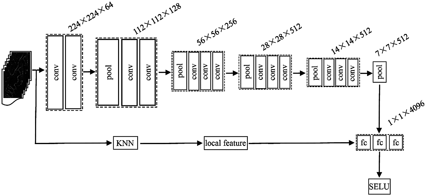
Figure 1: Framework of the proposed FL-CNN method
Fig. 1 shows that the proposed FL-CNN method includes a convolution layer, a pooling layer, and a full connection layer, in addition to the KNN embedded in the CNN network. The detailed process is follows:
Step 1. Input the original data and form a tensor with (n × 3) dimensions using the VGG16 model.
Step 2. Construct the local neighborhood of each point and obtain three feature graphs with (n × k) dimensions.
Step 3. Form 64 feature graphs with (n × k) dimensions after the convolution operation.
Step 4. Generate a feature vector with (1024 × 1) dimensions after the third pooling operation, which is classified by the full connection layer.
Step 5. Convert the output of the full connection layer by the scaled expected linear units function to the corresponding probability.
Compared with the other activation functions, the scaled expected linear units function has a stronger model robustness and scaling factor. The output of each layer of the CNN is automatically normalized to a Gaussian distribution with the mean value close to 0 and the variance close to 1.
The corresponding attribution probability of each category is defined as
where λ is the scale factor, λ = 1.05 and α = 1.67.
We conducted several experiments to evaluate the proposed LF-CNN method.
The proposed LF-CNN method was used with real open HSI remote sensing datasets. To improve the effectiveness and detection accuracy of the LF-CNN method, the HSI image dataset was pre-processed with geometric correction and image registration and then trained and tested on the computing platform. The LF-CNN method under the condition of small samples was then tested and evaluated on an HSI image, which has 115 channels ranging from 450 to 950 nm and covers (500 pixels × 500 pixels).
We used an HSI image representing a rural area. Fig. 2 shows the HSI false color composite image (Bands 68, 41, and 99). Based on a field survey, the rural areas were grouped into six classes corresponding to six categories of land cover (Classes 1–6).
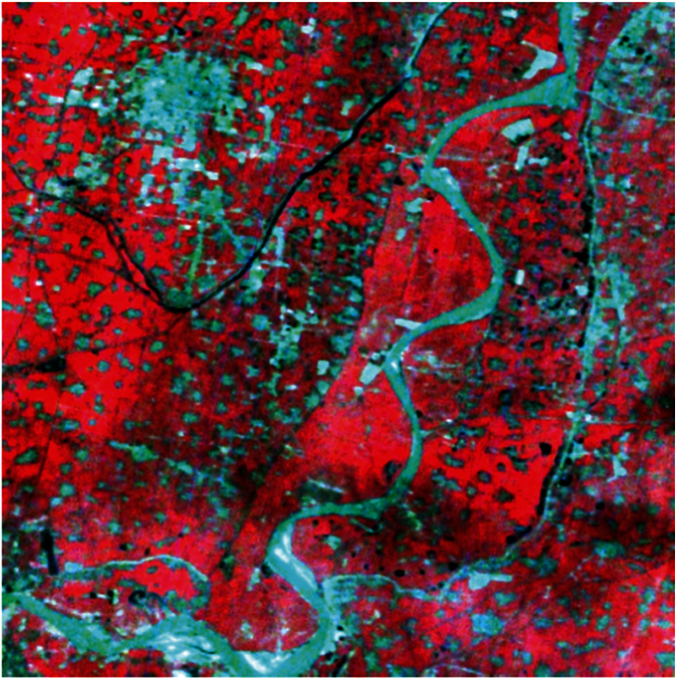
Figure 2: HSI false color composite image (bands 68, 41, and 99)
The spatial distribution characteristics of the HSI are predicted by the filter parameters learned in a fully convolutional network-8s (FCN-8s). The FCN-8s network in the VGG16 model not only better fits the nonlinear structure of the data and improves the expression of the model, but also reduces the computational complexity while maintaining the overall fitting cost. Based on detailed information about the front layer, it can obtain a more refined segmentation map by combining the local spatial features at multiple scales. This advantage is more obvious for data with a complex spatial structure. Compared with the existing extraction methods for spatial features based on deep learning, the FCN-8s is a pixel-level end-to-end feature learning structure. It is more flexible in spatial structure learning and has distinct advantages in computational complexity. Fig. 3 shows the spatial distribution of the HSI based on the FCN-8s/VGG16 model.
Fig. 3 shows that the 21 feature maps correspond to 21 neurons in the final prediction layer. Different targets can produce individual responses in each neuron and the addition of local feature information allows the network to extract better information about local details. Figs. 3a–3u show clear differences among the spatial distribution maps.
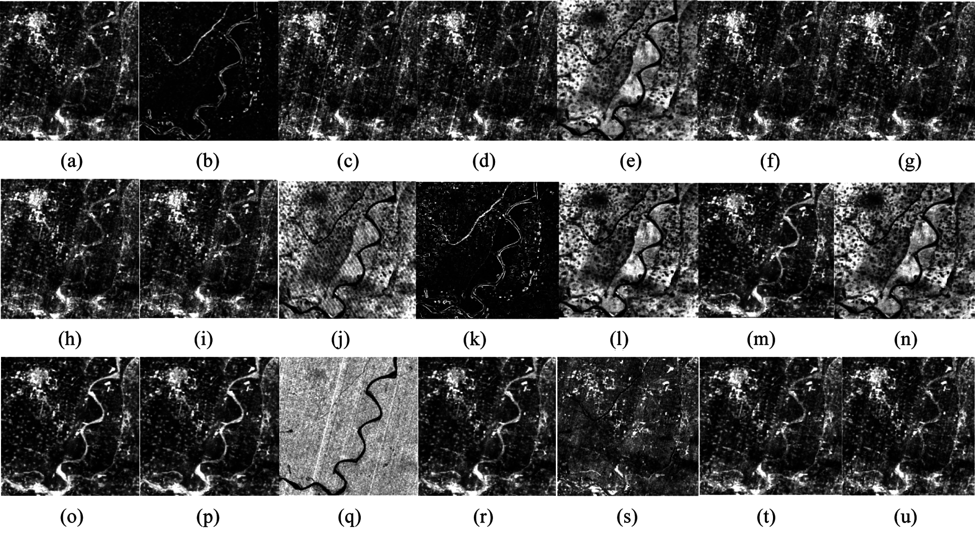
Figure 3: Spatial distribution of the HSI images based on FCN-8s/VGG16, (a)–(u) is the feature maps of the predicted spatial distribution in the HSI data, respectively.
The LF-CNN method was tested and implemented in Python 3.7, the deep learning framework of TensorFlow 2.0, trained in a CUDA-Toolkit 8.0 with an Intel Xeon E5-2620 v4 CPU, NVIDIA Quadro M4000 GPU and 8 GB of RAM, and a Linux Ubuntu 16.04 system installed on high-performance computers. The number of data samples was 2631, 2258, 1874, 2801, 728, and 1825 pixels, respectively. The adaptive moment estimation (Adam) was used to optimize the CNN model and the initial learning rate was 0.002, the momentum was 0.8, the batch size was 64, and the dropout rate was 0.5. In the network training, the initial weight W0 was initialized as a random number of Gaussian distributions and the initial deviation B0 was set to 0. The parameters of the trained FCN-8s network were migrated to extract the underlying structural information of the HSI data and the 21 feature maps of the last prediction layer in the FCN-8s network was regarded as the predicted spatial distribution of the HSI data.
4.3 Evaluation Index of Target Detection
The performance of proposed LF-CNN method was tested and evaluated by the overall accuracy (OA) and the kappa coefficient. To obtain more accurate evaluation results, the average classification results of 50 experiments were calculated and used for the statistical analysis.
The OA of target detection can be obtained by
where N is the total number of all the real reference pixels, xii is the diagonal of the confusion matrix and r represents the different types of target.
The kappa coefficient can be obtained by
where
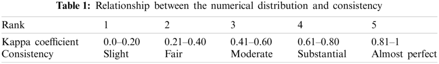
The range of the kappa coefficient is generally from −1 to 1. Table 1 shows the relationship between the numerical distribution of the kappa coefficient and consistency.
Figs. 4 and 5 show the training loss and accuracy, respectively, of the proposed LF-CNN method. The proposed LF-CNN method converges when the number of training samples reaches 500, when the target detection accuracy is highest and tends to be stable and the loss is low.
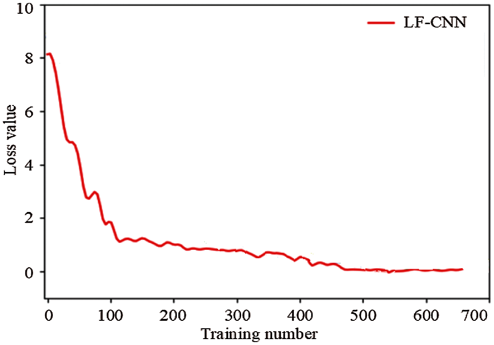
Figure 4: Training loss value curve of the LF-CNN method
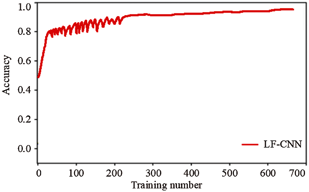
Figure 5: Training accuracy curve of the LF-CNN method
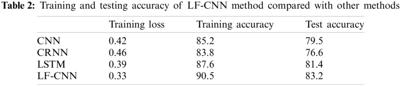
Table 2 shows the training and testing accuracy of proposed LF-CNN method compared with other methods. The accuracy of the proposed LF-CNN method reaches 90.5% on the training set and the loss reaches 0.33, both of which are better than the traditional CNN, CRNN, and LSTM methods. The accuracy of the proposed LF-CNN method reaches 83.2% in the test set, which is also better than the testing accuracy of the three earlier methods. This shows that the proposed LF-CNN method can effectively detect small sample targets from remote sensing images.
5.2 Influence of Different k Value
In constructing the local neighborhood using the KNN method, the local structure with k nearby points is different, which will affect the detection and classification of small sample targets. Table 3 shows the small sample target detection accuracy of the LF-CNN method under different k-value conditions.
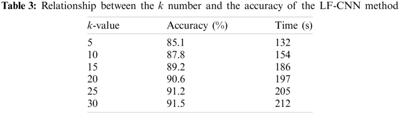
Table 3 shows that with an increase in the number of adjacent k-value points, the overall classification accuracy of the proposed LF-CNN method is continuously improved and the increased range of the total accuracy gradually decreases. To avoid the impact of the small number of local features on the recognition and classification results, the local neighborhood must contain a certain number of features during construction. However, with an increase in the k-value, both the local neighborhood and the training time increase.
5.3 Comparison of Different Methods
To obtain more accurate feature extraction information, the local feature is extracted and fused to the CNN model to reach the global features. To some extent, this clarifies the boundary location of low-resolution data. Fig. 6 shows the classification results for HSI remote sensing images obtained using different methods.
The traditional CNN, CRNN, and LSTM models were introduced to evaluate the classification accuracy of the proposed LF-CNN method (Table 4). The LF-CNN method produced the highest overall classification accuracy on the HSI data of about 90.32% and the kappa coefficient reached 0.8792. The LF-CNN method produced good classification results based on Table 1. The LF-CNN method had a clear classification advantage compared with the CNN, CRNN, and LSTM methods. From the perspective of targets, the accuracy of the single category target information obtained by the LF-CNN method was better than the single classification effect of other methods. Among the different types of target information, the detection results for Classes 4 and 5 were confused, whereas the degree of confusion was weak in the other categories. This is mainly because the spectral characteristics of the ground objects in Classes 4 and 5 were similar, which can lead to misclassification. This is consistent with Figs. 6b and 6c. Although the confusion between Classes 4 and class 5 was serious, the proposed LF-CNN method can achieve a high classification accuracy and ensure spatial consistency at a high level.
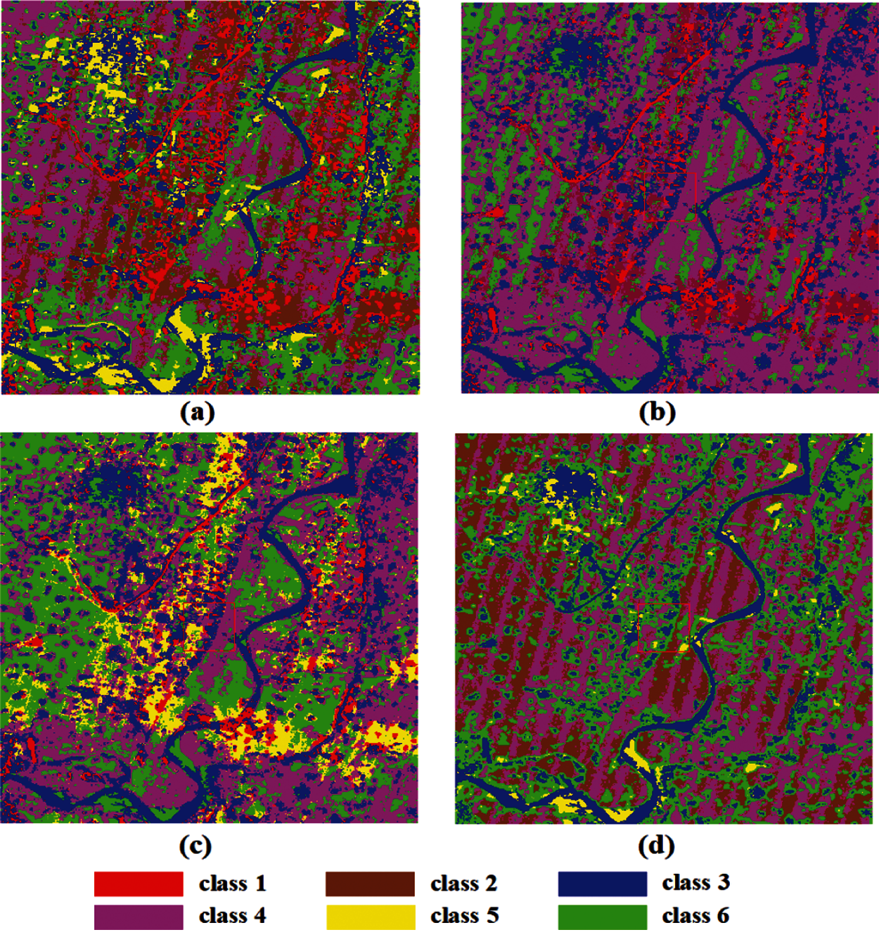
Figure 6: Classification results of HSI remote sensing images. (a) LF-CNN, (b) CNN, (c) CRNN, and (d) LSTM
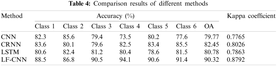
Table 5 compares the operational time in different experiments. The average value of 50 experiments was counted as the operation time under different sample sizes.
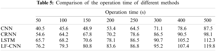
Table 5 shows that the proposed LF-CNN method requires a longer operation time than the CNN, CRNN, and LSTM methods. This is mainly because the radius of the optimum neighborhood window is small in the LF-CNN method. Under the condition of small samples, the disadvantage of many repeated calculations gradually becomes more important and the computational complexity increases sharply. This is clearly seen when the sample size of each category is <400. The proposed LF-CNN method has a slightly higher time complexity than the other three methods, but the running time does not increase sharply with increasing sample size. The gap is therefore within an acceptable range under normal circumstances.
5.5 Influence of Different Sample Size
Fig. 7 shows the classification accuracy of different methods as the number of training samples changes. Fig. 7 shows that under the condition of small samples, particularly a small number of training samples, the classification accuracy of the proposed LF-CNN method is significantly better than that of the CNN, CRNN, and LSTM methods. The classification accuracy of the different methods also gradually increases with an increase in the number of training samples. The classification accuracy of different methods gradually becomes stable when the number of samples reaches 500.
The classification accuracy of the LF-CNN method reaches 97% when the number of training samples reaches 200. The LSTM method achieves the highest classification accuracy of the different methods for the same number of the training sample conditions. A greater number of training samples is required to achieve the highest classification accuracy for the CNN and CRNN methods than for the LF-CNN and LSTM methods. The classification accuracy of the different methods does not increase significantly with an increase in sample size. This shows the applicability and accuracy of the proposed LF-CNN method under small samples conditions.
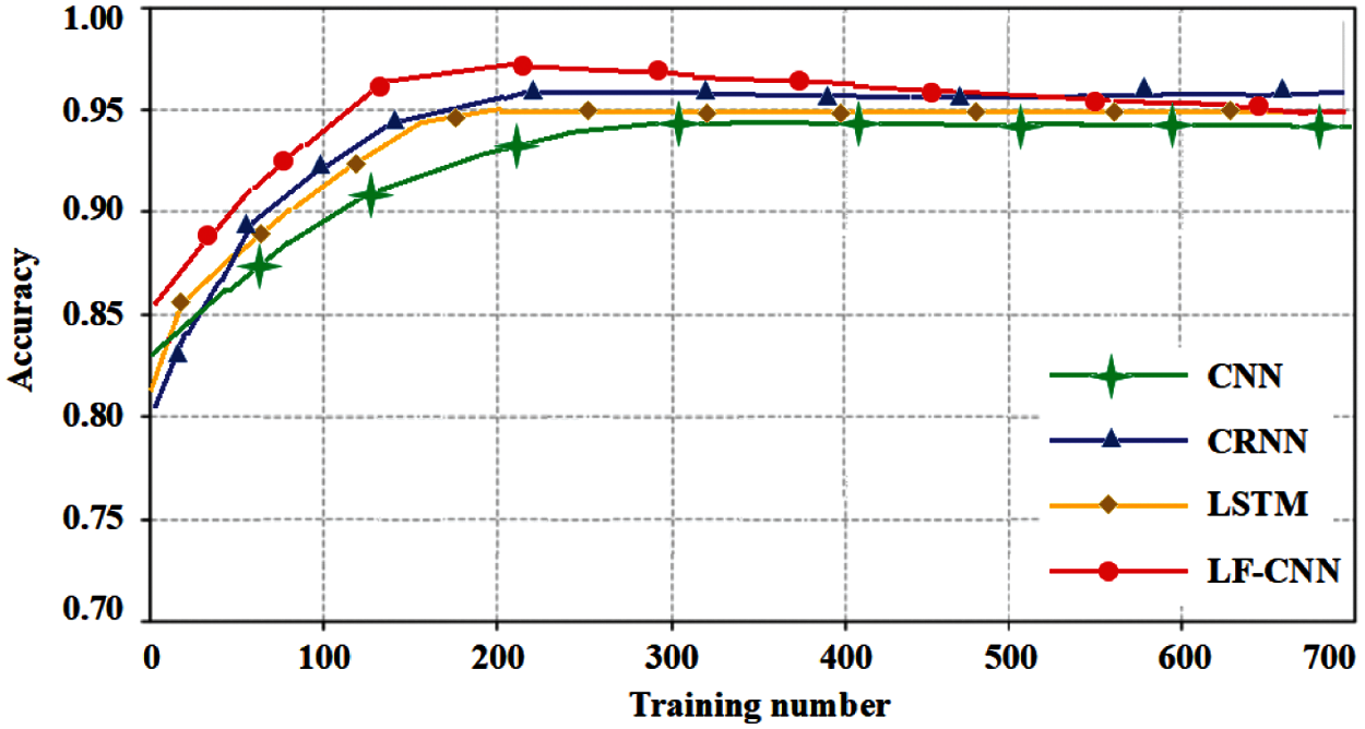
Figure 7: Relation between the accuracy of different methods and the number of training samples
The distribution of target samples is usually unbalanced in remote sensing images and the number of samples is small, limiting classification. The rapid development of deep learning techniques has brought new ideas to small sample target detection in remote sensing images. The excellent performance of the CNN method in optical images has led to its application in the classification of remote sensing images. We used the LF-CNN method in combination with local features and CNN to detect small numbers of sample targets and verified our method with HSI remote sensing images. The proposed LF-CNN method significantly improved the accuracy of small sample target recognition and detection in remote sensing images compared with traditional remote sensing classification methods via the fusion of local features.
This work provides useful results for small sample target detection. Our main conclusions are as follows:
(1) We fused local features into the VGG16 model. The proposed LF-CNN method refines the edge detection ability of the CNN model for low-resolution images.
(2) We verified the proposed LF-CNN method in terms of algorithm performance, k-value, time complexity, and sample size. The method is both practical and accurate.
(3) We introduced the LF-CNN method into the HSI remote sensing classification to expand the range of application of the traditional CNN method.
Although the proposed LF-CNN method achieved good accuracy in target detection and the classification of HSI remote sensing images, the calculations are time consuming and the selection of the model parameters and the k-value require further optimization. The design and performance verification of this model were mainly carried out on HSI remote sensing images and we need to verify whether it is applicable to other high- and medium-resolution remote sensing datasets. The proposed LF-CNN model only has a few layers and it is difficult to extract deeper target information features. An increased number of layers in the network model is required but without significantly increasing the amount and complexity of computation. We plan to carry out new experiments and tests in these areas.
Acknowledgement: The authors wish to express their appreciation to the Shanghai Engineering Research Center of Intelligent Computing System and the reviewers for their helpful suggestions which greatly improved the presentation of this paper.
Funding Statement: This work was partially supported by the Key Laboratory for Digital Land and Resources of Jiangxi Province, East China University of Technology (DLLJ202103), and Science and Technology Commission Shanghai Municipality (No. 19142201600), Graduate Innovation and Entrepreneurship Program in Shanghai University in China (No. 2019GY04).
Conflicts of Interest: The authors declare that they have no conflicts of interest to report regarding the present study.
1. Reese, D. C., O’Malley, R. T., Brodeur, R. D., Churnside, J. H. (2019). Epipelagic fish distributions in relation to thermal fronts in a coastal upwelling system high-resolution remote-sensing technique. ICES Journal of Marine Science, 68(9), 1865–1874. DOI 10.1093/icesjms/fsr107.1865. [Google Scholar] [CrossRef]
2. Yi, W. B., Tang, H., Chen, Y. H. (2011). An object-oriented semantic clustering algorithm for high-resolution remote sensing images using the aspect model. IEEE Geoscience and Remote Sensing Letters, 8(3), 522–526. DOI 10.1109/LGRS.2010.2090034. [Google Scholar] [CrossRef]
3. Sanchez-Azofeifa, A., Rivard, B., Wright, J., Feng, J. L., Li, P. J. et al. (2018). Estimation of the distribution of Tabebuia guayacan (Bignoniaceae) using high-resolution remote sensing imagery. Sensors, 11(4), 3831–3851. DOI 10.3390/s110403831. [Google Scholar] [CrossRef]
4. Chen, S. P., Tong, Q. H., Guo, H. D. (1998). Mechanism of remote sensing information. Beijing: China Science Press. [Google Scholar]
5. Chang, C. L. (2003). Hyperspectral imaging: Techniques for spectral detection and classification. New York: Kluwer Academic/Plenum Publishers. [Google Scholar]
6. Mallinis, G., Koutsias, N., Tsakiri-strati, M., Karteris, M. (2007). Object-based classification using quickbird imagery for delineating forest vegetation polygons in a mediterranean test site. Journal of Photogrammetry & Remote Sensing, 63(2), 237–250. DOI 10.1016/j.isprsjprs.2007.08.007. [Google Scholar] [CrossRef]
7. Chen, X. Q., Chen, S. P., Zhou, C. H. (2006). Segmentation approach for remote sensing images based on local homogeneity gradient and its evaluation. Journal of Remote Sensing, 10(3), 357–365. DOI 10.3321/j.issn:1007-4619.2006.03.012. [Google Scholar] [CrossRef]
8. Bai, M., Liu, H. P., Qiao, Y., Wang, X. D. (2010). New progress in the classification of high spatial resolution satellite images for LUCC. Remote Sensing for Land & Resources, 22(1), 19–23. DOI 10.3724/SP.J.1146.2009.01622. [Google Scholar] [CrossRef]
9. Radoux, J., Defourny, P. A. (2007). A quantitative assessment of boundaries in automated forest stand delineation using very high-resolution imagery. Remote Sensing of Environment, 110(4), 468–475. DOI 10.1016/j.rse.2007.02.031. [Google Scholar] [CrossRef]
10. Foody, G. M. (1997). Fully fuzzy supervised classification of land cover from remotely sensed imagery with an artificial neural network. Neural Computing & Applications, 5(4), 238–247. DOI 10.1007/BF01424229. [Google Scholar] [CrossRef]
11. Mackin, K. J., Nunohiro, E., Ohshiro, M., Yamasaki, K. (2006). Land cover classification from MODIS satellite data using probabilistically optimal ensemble of artificial neural networks. Lecture Notes in Computer Science, 232(3), 820–826. DOI 10.1007/11893011. [Google Scholar] [CrossRef]
12. Mokhtarzade, M., Valadan Zoej, M. J. (2007). Road detection from high-resolution satellite images using artificial neural networks. International Journal of Applied Earth Observation and Geoinformation, 9(1), 32–40. DOI 10.1016/j.jag.2006.05.001. [Google Scholar] [CrossRef]
13. Luo, J. C., Zhou, C. H., Yang, Y. (2001). ANN remote sensing classification model and its integration approach with geo-knowledge. Journal of Remote Sensing, 5(2), 121–129. DOI 10.3321/j.issn:1007-4619.2001.02.010. [Google Scholar] [CrossRef]
14. She, X. Y., Xue, H. F., Lei, X. W., Tang, G. A. (2006). The remote sensing image classification research based on mining classification rules on the spatial database. Journal of Remote Sensing, 10(3), 332–338. DOI 10.1360/aps040087. [Google Scholar] [CrossRef]
15. Zhang, W. G., Li, H. R., Wu, C. Z., Wang, L. (2021). Stability assessment of underground entry-type extractions using data-driven RF and KNN methods. Journal of Hunan University (Natural Sciences), 48(3), 164–172. DOI 10.16339/j.cnki.hdxbzkb.2021.03.017. [Google Scholar] [CrossRef]
16. Yakowitz, S. (1987). Nearest-neighbor methods for time series analysis. Journal of Time Series Analysis, 8(2), 235–247. DOI 10.1111/j.1467-9892.1987.tb00435.x. [Google Scholar] [CrossRef]
17. Lan, Q. J., Li, W. K., Liu, W. X. (2016). Performance and choice of Chinese text classification models in different situations. Journal of Hunan University (Natural Sciences), 43(4), 141–146. DOI 10.16339/j.cnki.hdxbzkb.2016.04.019. [Google Scholar] [CrossRef]
18. Li, H. (2012). Statistical learning methods. Beijing: Tsinghua University Press. [Google Scholar]
19. Kang, S. K. (2021). K-nearest neighbor learning with graphic neural networks. Mathematics, 9(8), 830. DOI 10.3390/math9080830. [Google Scholar] [CrossRef]
20. Sun, Y. K., Lin, Q. Z., He, X., Zhao, Y. J., Dai, F. et al. (2021). Wood species recognition with small data: A deep learning approach. International Journal of Computational Intelligence Systems, 14(1), 1451–1460. DOI 10.2991/ijcis.d.210423.001. [Google Scholar] [CrossRef]
21. Ye, L. H., Wang, L., Zhang, W. W., Li, Y. G., Wang, Z. K. (2019). Deep metric learning method for high resolution remote sensing image scene classification. Acta Geodaetica et Cartographica Sincia, 48(6), 698–707. DOI 10.11947/j.AGCS.2019.20180434. [Google Scholar] [CrossRef]
22. Yu, T., Yang, J. (2020). Point cloud model recognition and classification based on K-nearest neighbor convolutional neural network. Laser & Optoelectronics Progress, 57(10), 101510. DOI 10.3788/LOP57.101510. [Google Scholar] [CrossRef]
23. Borgi, A., Akdag, H. (1999). Knowledge based supervised classification: An application to image processing. Proceedings of the EUSFLAT-ESTYLF Joint Conference, pp. 175–178. Palma de Mallorca, Spain. [Google Scholar]
24. Habib, T., Inglada, J., Mercier, G., Chanussot, J. (2009). Support vector reduction in SVM algorithm for abrupt change detection in remote sensing. IEEE Geoscience and Remote Sensing Letters, 6(3), 606–610. DOI 10.1109/LGRS.2009.2020306. [Google Scholar] [CrossRef]
25. Maulik, U., Chakraborty, D. (2019). A self-trained ensemble with semisupervised SVM: An application to pixel classification of remote sensing imagery. Pattern Recognition, 44(3), 615–623. DOI 10.1016/j.patcog.2010.09.021. [Google Scholar] [CrossRef]
26. Mountrakis, G., Irn, J., Ogole, C. (2018). Support vector machines in remote sensing: A review. ISPRS Journal of Photogremmetry and Remote Sensing, 66(3), 247–259. DOI 10.1016/j.isprsjprs.2010.11.001. [Google Scholar] [CrossRef]
27. Li, F. F., Fergus, R., Perona, P. (2003). A Bayesian approach to unsupervised one-shot learning of object categories. Proceeding of the IEEE International Conference on Computer Vision, pp. 1134–1141. Nice, France. [Google Scholar]
28. Li, F. F., Fergus, R., Perona, P. (2006). One-shot learning of object categories. IEEE Transaction on Pattern Analysis & Machine Intelligence, 28(4), 594–611. DOI 10.1109/TPAMI.2006.79. [Google Scholar] [CrossRef]
29. Lake, B. M., Salakhutdinov, R., Tenenbaum, J. B. (2015). Human-level concept learning through probabilistic program induction. Science, 350(6266), 1332–1338. DOI 10.1126/science.aab3050. [Google Scholar] [CrossRef]
30. Schwartz, E., Karlinsky, L., Shtok, J., Harary, S., Marder, M. et al. (2018). Delta-encoder: An effective sample synthesis method for few-shot object recognition. Proceeding of the 32nd International Conference on Neural Information Processing System, pp. 2845–2855. Montréal, Canada. [Google Scholar]
31. Bartunov, S., Vetrov, D. P. (2018). Few-shot generative modelling with generative matching networks (supplementary materials). Proceeding of the 21th International Conference on Artificial Intelligence and Statistics, pp. 670–678. Lanzarote, Spain. [Google Scholar]
32. Zhang, R., Che, T., Ghahramani, Z., Bengio, Y., Song, Y. Q. (2018). MetaGAN: An adversarial approach to few-shot learning. Proceeding of the 32nd International Conference on Neural Information Processing System, pp. 2371–2380. Montréal, Canada. [Google Scholar]
33. Koch, G., Zemel, R., Salakhutdinov, R. (2015). Siamese neural networks for one-shot image recognition. Proceeding of the 32nd International Conference on Machine Learning, pp. 2–15. Lille, France. [Google Scholar]
34. Vinyals, O., Blundell, C., Lillicrap, T., Kavukcuoglu, K., Wierstra, D. (2016). Matching networks for one shot learning. Proceeding of the 30nd International Conference on Neural Information Processing System, pp. 3630–3638. Barcelona, Spain. [Google Scholar]
35. Snell, J., Swersky, K., Zemel, R. (2017). Prototypical networks for few-shot learning. Proceeding of the 31nd International Conference on Neural Information Processing System, pp. 4077–4087. Long Beach, USA. [Google Scholar]
36. Sung, F., Yang, Y., Zhang, L., Xiang, T., Torr, P. H. S. et al. (2017). Learning to compare: Relation network for few-shot learning. Proceeding of the 30th IEEE/CVF Conference on Computer Vision and Pattern Recognition, pp. 1199–1208. Salt Lake City, USA. [Google Scholar]
37. Li, W., Xu, J., Huo, J., Wang, L., Luo, J. (2019). Distribution consistency based covariance metric networks for few-shot learning. Proceeding of the 33th AAAI Conference on Artificial Intelligence, pp. 458–472. Honolulu, USA. [Google Scholar]
38. Ravi, S., Larochelle, H. (2017). Optimization as a model for few-shot learning. Proceeding of the International Conference on Learning Representations, pp. 1–11. Toulon, France. [Google Scholar]
39. Finn, C., Abbeel, P., Levine, S. (2017). Model-agnostic meta-learning for fast adaptation of deep networks. Proceeding of the 34th International Conference on Machine Learning, pp. 1126–1135. Sydney, Australia. [Google Scholar]
40. Ravichandran, A., Bhotika, R., Soatto, S. (2019). Few-shot learning with embedded class models and shot-free meta training. Proceeding of the International Conference on Computer Vision, pp. 331–339. Seoul, Korea. [Google Scholar]
41. Sun, Q., Liu, Y., Chua, T., Schiele, B. (2019). Meta-transfer learning for few-shot learning. Proceeding of the 32th IEEE/CVF Conference on Computer Vision and Pattern Recognition, pp. 403–412. Long Beach, USA. [Google Scholar]
42. Chen, W., Liu, Y., Kira, Z., Wang, Y. C. F., Huang, J. B. (2019). A closer look at few-shot classification. Proceeding of the International Conference on Learning Representation, pp. 542–551. New Orleans, USA. [Google Scholar]
43. Ruwali, A., Kumar, A. J. S., Prakash, K. B., Sivavaraprasad, G., Ratnam, D. V. (2021). Implementation of hybrid learning model (LSTM-CNN) for lonospheric TEC forecasting using GPS data. IEEE Geoscience and Remote Sensing Letters, 18(6), 1004–1008. DOI 10.1109/LGRS.2020.2992633. [Google Scholar] [CrossRef]
44. Chen, H., Wang, Y., Wang, G. Y., Qiao, Y. (2018). LSTD: A low-shot transfer detector for object detection. Proceeding of the 32th AAAI Conference on Artificial Intelligence, pp. 258–274. New Orleans, USA. [Google Scholar]
45. Dong, X., Zheng, L., Ma, F., Yang, Y., Meng, D. Y. (2018). Few-example object detection with model communication. IEEE Transaction on Pattern Analysis & Machine Intelligence, 41(7), 641–1654. DOI 10.1109/TPAMI.2018.2844853. [Google Scholar] [CrossRef]
46. Wang, T., Zhang, X., Yuan, L., Feng, J. (2019). Few-shot adaptive faster R-CNN. Proceeding of the 32th IEEE/CVF Conference on Computer Vision and Pattern Recognition, pp. 7173–7182. Long Beach, USA. [Google Scholar]
47. Karlinsky, L., Shtok, J., Harary, S., Schwartz, E., Bronstein, A. M. (2019). RepMet: Representative-based metric learning for classification and few-shot object detection. Proceeding of the 32th IEEE/CVF Conference on Computer Vision and Pattern Recognition, pp. 5197–5206. Long Beach, USA. [Google Scholar]
48. Kang, B., Liu, Z., Wang, X., Yu, F., Feng, J. et al. (2019). Few-shot object detection via feature reweighting. Proceeding of the International Conference on Computer Vision, pp. 8420–8429. Seoul, Korea. [Google Scholar]
 | This work is licensed under a Creative Commons Attribution 4.0 International License, which permits unrestricted use, distribution, and reproduction in any medium, provided the original work is properly cited. |