| Computer Modeling in Engineering & Sciences |
DOI: 10.32604/cmes.2022.018965
ARTICLE
Visualization Detection of Solid–Liquid Two-Phase Flow in Filling Pipeline by Electrical Capacitance Tomography Technology
1College of Electrical and Control Engineering, Xi'an University of Science and Technology, Xi'an, 710054, China
2College of Energy Engineering, Xi'an University of Science and Technology, Xi'an, 710054, China
*Corresponding Author: Lang Liu. Email: liulang@xust.edu.cn
Received: 26 August 2021; Accepted: 15 October 2021
Abstract: During mine filling, the caking in the pipeline and the waste rock in the filling slurry may cause serious safety accidents such as pipe blocking or explosion. Therefore, the visualization of the inner mine filling of the solid–liquid two-phase flow in the pipeline is important. This paper proposes a method based on capacitance tomography for the visualization of the solid–liquid distribution on the section of a filling pipe. A feedback network is used for electrical capacitance tomography reconstruction. This reconstruction method uses radial basis function neural network fitting to determine the relationship between the capacitance vector and medium distribution error. In the reconstruction process, the error in the linear back projection is removed; thus, the reconstruction problem becomes an accurate linear problem. The simulation results show that the reconstruction accuracy of this algorithm is better than that of many traditional algorithms; furthermore, the reconstructed image artifacts are fewer, and the phase distribution boundary is clearer. This method can help determine the location and size of the caking and waste rock in the cross section of the pipeline more accurately and has great application prospects in the visualization of filling pipelines in mines.
Keywords: Electrical capacitance tomography; mine backfilling; visualization detection; image reconstruction; radial basis function neural network
In the process of mining, cemented tailing filling technology is often adopted to reduce environmental pollution and solve problems such as surface subsidence [1]. The slurry of the mine filling body is a solid–liquid two-phase flow that contains tailings, waste rock, cementing material, water, and other components, which flows in a complex manner in the filling pipeline [2]. During transportation, owing to pressure change, pipe distribution position, and other factors, problems such as internal deposition, scaling, and blockage of pipelines can easily occur, which can affect the safety of the filling pipeline and the mine filling process. To avoid the blockage of the filling pipeline and reduce the detection cost, the visual detection of the pipeline has attracted increasing attention [3]. Liu et al. [4] proposed the use of electrical resistance tomography technology to detect the filling pipeline, but there was no considerable imaging effect. Electrical capacitance tomography (ECT) technology can help visualize the phase distribution in a pipeline cross-section and obtain reliable and intuitive results for pipeline detection.
ECT, a nondestructive testing method, is an effective means to monitor multiphase flow. As the permittivity of the medium in the measured pipeline may vary, ECT can calculate the permittivity distribution from the measured capacitance through the reconstruction algorithm, which can reflect the corresponding phase distribution [5]. Based on the different computing principles of reconstruction, reconstruction algorithms can be classified as non-iterative and iterative algorithms. Linear back projection (LBP) [6] and Tikhonov regularization [7] are examples of non-iterative algorithms, whereas the Newton-Raphson algorithm [8] and the algebraic reconstruction technique (ART) [9] are iterative algorithms. Non-iterative algorithms are fast but have poor accuracy. Although iterative algorithms have high accuracy, their effect is still not ideal. Owing to the soft field effect of the reconstruction problem, there is a nonlinear relationship between the measured capacitance and the distribution of the dielectric constant. However, all of the above algorithms are linear reconstruction algorithms, which perform calculations based on the linear relationship. Therefore, linearization errors are introduced in the reconstruction, which results in a decrease in accuracy [10–12]. In recent years, many researchers have applied the fitting and prediction capabilities of neural networks to reconstruction algorithms. Li et al. [13] proposed a reconstruction algorithm based on a radial basis function neural network (RBFNN). The reconstruction speed is high, the effect is satisfactory, and it has a certain practical value. Tian et al. [14] established an image reconstruction framework using the radial basis function and the sparsity of the phase distribution. Zhu et al. [15] developed a deep convolutional neural network and adopted a mixed training strategy to map the capacitance to the permittivity distribution. Zheng et al. [16] developed a self-encoder neural network using a fully connected network to solve the image reconstruction problem of ECT. Yang et al. [17] further optimized the reconstructed image based on the U-Net framework. Wang et al. [18] inputted the results of Landweber iterative reconstruction into a two-channel convolutional neural network, which improved the feature extraction capability of the network and the reconstruction effect of the image details.
In this study, an ECT reconstruction feedback network based on an RBFNN was established, and the center selection of the RBFNN was realized using the orthogonal least squares (OLS) algorithm. There are major errors in the calculation results of linear reconstruction algorithms. Using a feedback reconstruction network, the errors were removed, and accurate imaging results were obtained.
In Section 2, the system model and mathematical principle of capacitance tomography are introduced. Section 3 describes the proposed ECT feedback network reconstruction method, the RBFNN, and the training dataset. In Section 4, the corresponding experiments and results are presented. Section 5 presents a summary and prospects for future research.
In this study, an ECT system was investigated and verified through simulation experiments. The ECT system is illustrated in Fig. 1. This system consists of a 12-electrode ECT sensor, a capacitance measurement circuit, and an upper computer (PC).
Figure 1: ECT system
The 12-electrode ECT system was studied, and there were 66 independent measured capacitance values. Fig. 1 shows the ECT sensor. In the two-dimensional ECT model shown in Fig. 2, 12 electrodes are distributed on the outside of the pipe and close to the pipe wall; furthermore, a shield is used to reduce interference from the outside of the system, and there are two different media in the pipe under test.
Figure 2: ECT sensor model
In the capacitance tomography system, there is a nonlinear relationship between the capacitance C between the plates and the dielectric constant
where V is the potential difference between the corresponding plates,
where
Because the number of pixels required for imaging is much larger than the number of measured capacitance values, the dimension of g is much larger than that of C. The number of calculations required for sensitivity S will increase with an increase in the precision of the sensitive field partition. Because the condition number of S is large, the disturbance with a small measured capacitance value will cause a large change in the dielectric constant [20]. Therefore, the solution to the inverse problem based on Eq. (2) is inconclusive.
To address these problems, this paper proposes the use of an RBFNN to establish the nonlinear relationship between capacitance and dielectric constant values and to select the center of the RBFNN using the OLS method.
3 Reconstruction Algorithm and Training Samples
In this study, the LBP reconstruction algorithm was used to solve the ECT inverse problem, and an RBFNN was used to realize the nonlinear mapping between the approximation measurement capacitance and LBP reconstruction error. An OLS was used to optimize the RBFNN. Thus, the ECT feedback network was implemented. This section introduces the overall framework of the ECT feedback network based on the RBFNN, the principle of OLS-RBF, and the generation of the training set.
In the LBP algorithm, the solution of the dielectric constant value is expressed as follows:
where
Hypothesis
which can be obtained through Eq. (4) as follows:
If the nonlinear relationship between the measured capacitance and the reconstruction error is known, the error generated by Eq. (3) can be reduced using Eq. (6) to improve the reconstruction accuracy.
An RBFNN based on the OLS algorithm was established to realize the nonlinear mapping between the measured capacitance and the reconstruction error. The feedback ECT reconstruction method based on the RBFNN proposed in this paper is shown in Fig. 3, where C represents the capacitance vector, G represents the original image in the training set,
Figure 3: Structure of ECT feedback network
An RBFNN has a feedforward structure with a single hidden layer, and the application of its kernel function can map low-dimensional linearly indivisible data to high-dimensional space, making it linearly separable in a high-dimensional space [21]. Owing to its local approximation ability and nonlinear characteristics, it can approximate the continuous function of arbitrary accuracy. Owing to the inaccuracy of the inverse problem of ECT and the nonlinearity of the distribution of capacitance as well as the media constant, the reconstruction of the LBP algorithm will result in major errors. The proposed reconstruction algorithm uses the trained RBFNN to predict such errors and eliminate them in the reconstruction process in order to realize an accurate calculation of the media distribution. The structure of the RBFNN is shown in Fig. 4. The input of the network is the capacitance vector, and the output is the predicted IE.
Figure 4: Structure of RBF network
The RBFNN takes neurons as nodes and the radial basis function as the excitation function. The activation function of the hidden layer node responds locally to the input. When the input is close to the central range of the base function, the hidden layer node will produce a large output; when the input is far from the central point, the output decays exponentially. The hidden layer neurons obtain the output layer by linear addition.
RBFs are non-negative real-valued functions whose values depend on the input distance from the central point and are radially symmetric. The Gaussian function is expressed as follows:
where x is the input,
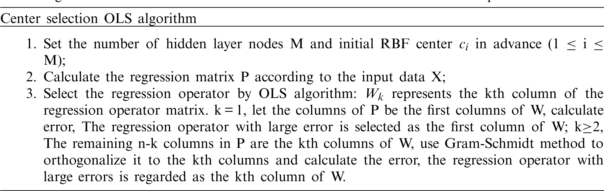
When using an RBFNN, the most important factor is selecting the center point. In this study, the OLS algorithm was used to select the center and construct the RBFNN. RBF network can be viewed as the following regression model:
where,
OLS transforms the P set into orthogonal basis vectors, and then obtains the effect of each basis vector on the output,
where, A is an upper triangular matrix in M dimension with diagonal 1, W is an N × M matrix, and
where H is a diagonal matrix whose diagonal element is
where, g in OLS algorithm is represented as
The gram-Schmidt method can be used to obtain the value of the least squares estimate
COMSOL Multiphysics finite element software was used to establish four distributions of ECT models: single-core, two-core, three-core, and stratified. When modeling different samples in COMSOL, different parameters were used to describe their characteristics. Figs. 5a–5c show the core distribution, and the parameters describing the sample are the center position and radius. Fig. 5d shows the stratified distribution, and its parameters are the height of the stratified distribution interface and the inclination angle between the normal line of the interface and the horizontal line. Different samples can be created by generating random parameters.
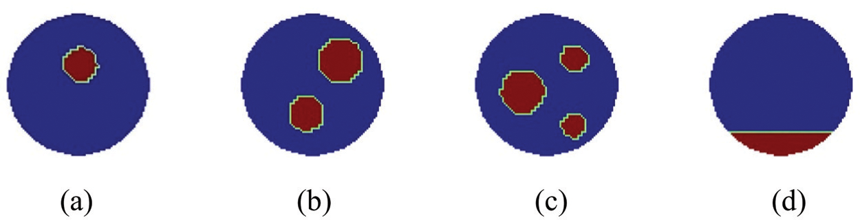
Figure 5: Training samples (a) Single-core (b) Two-core (c) Three-core (d) Stratified
Each distribution sample was simulated by COMSOL to obtain 5,000 datasets, with a total of 20,000 data sets. Each dataset consists of a measured capacitance vector C and a dielectric constant value vector g. C and g are the input and expected output of the network, respectively. To accelerate the convergence speed of the network training, before using the data set to train the network, each group of measured capacitance values needs to be normalized. The normalization formula for C is as follows:
where
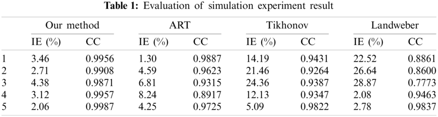
To verify the effectiveness of the proposed reconstruction method, two criteria of correlation coefficient (CC) and image error (IE) are used to quantitatively evaluate the reconstruction accuracy:
where G represents the distribution of the dielectric constant of the original image, G represents the distribution of the dielectric constant of the reconstructed image,
Fig. 6 shows the reconstruction results of noiseless data calculated by the proposed algorithms, ART algorithm, Tikhonov algorithm, and Landweber iterative method. Table 1 shows the IE and CC, corresponding to the results in Fig. 6. For the reconstruction results, our algorithm had a lower IE, higher CC, and better imaging effect. The reconstruction results show that the proposed algorithm can significantly reduce artifacts in the reconstruction results in all cases and more accurately display the position where the phase distribution changes; it also achieves high reconstruction accuracy. The ART algorithm has a good reconstruction effect for the core flow, but it cannot obtain the exact reconstruction results for the laminar flow distribution. The Tikhonov and Landweber algorithms perform better on laminar flow than ART, but they cannot eliminate artifacts in the core flow reconstruction results. Because the nonlinearity of the ECT inverse problem is removed in the reconstruction process, the reconstruction results are closer to the real permittivity distribution, and there are fewer artifacts.
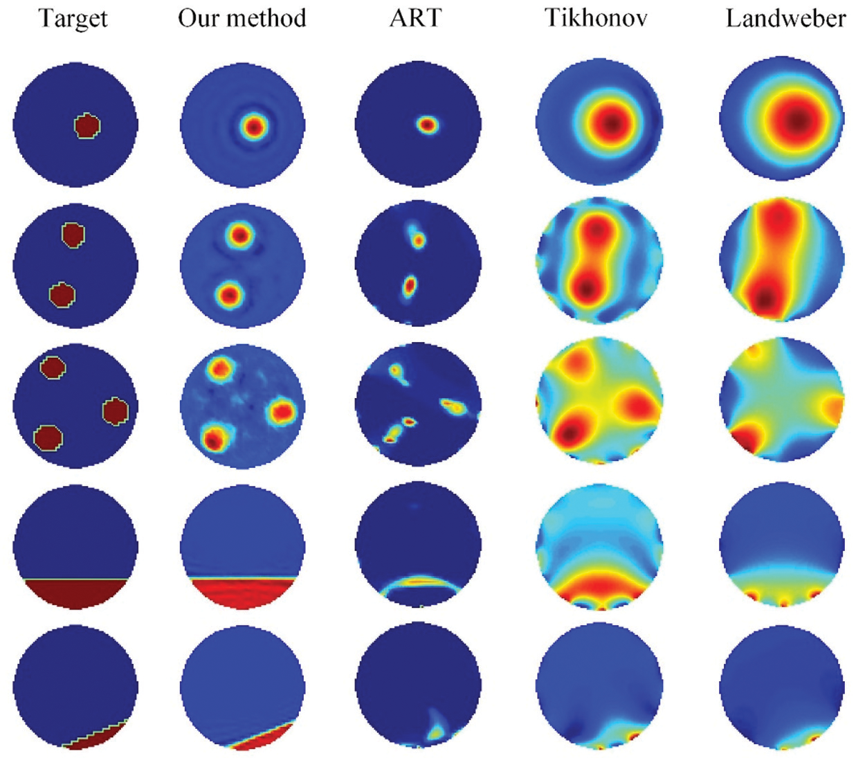
Figure 6: Comparison of simulation experiments
To further study the anti-noise performance of the algorithm, the capacitance data are added to the noise and then inputted to the feedback reconstruction network for calculation. The signal-to-noise ratio (SNR) is expressed as follows:
where,
Noise was added to the capacitor vector, as shown in Fig. 7. First, the capacitance matrix was expanded, and then Gaussian noise with a preset SNR (SNR = 50) was added to each row of the expanded matrix. Any column of the expanded matrix can be used as a result of the added noise. Gaussian noise with a preset SNR (SNR = 50) was added to each row.
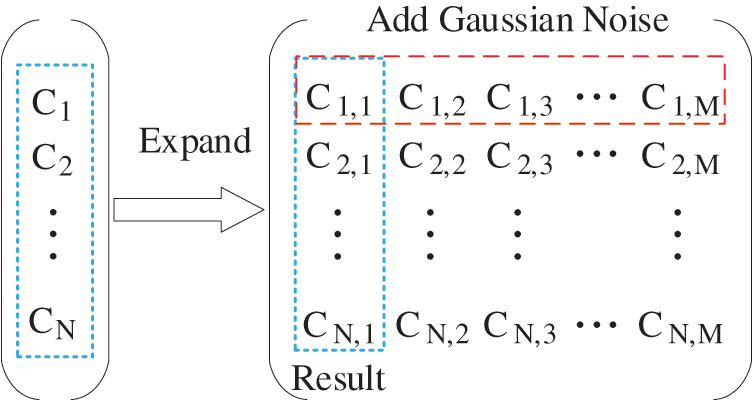
Figure 7: Processes of noise-contaminated capacitance generation
Fig. 8 shows the reconstruction results for the noisy data. The proposed algorithm still has a good imaging effect when the capacitance data are polluted by noise. Thus, the proposed reconstruction method has strong noise resistance and good generalization ability; furthermore, the reconstruction effect is satisfactory. The proposed method can be used for the visualization of filling pipelines based on ECT technology.
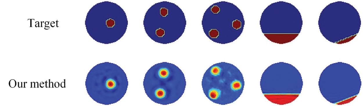
Figure 8: Reconstruction results based on noise-contaminated simulation data
A feedback reconstruction network based on an RBFNN was proposed for mine filling pipeline visualization and to reduce the error caused by nonlinearity in the ECT reconstruction process. After the calculation error caused by the linear algorithm is removed from the model, the ECT reconstruction problem is transformed from nonlinear to linear inverse. In this study, typical two-phase flow data samples were used to train the RBFNN for predicting the reconstruction error, and the LBP algorithm was used to complete the image reconstruction. In the simulation results, for the data without noise and the data interfered by noise, the proposed reconstruction method has a high reconstruction accuracy, fewer imaging artifacts, and a clear phase distribution boundary. It can effectively judge the caking and blockage in the pipeline, which has an important application prospect. The feedback reconstruction network greatly reduces the error of the linear model of ECT. It can be combined with a more complex reconstruction algorithm to further improve the accuracy of the reconstruction algorithm, providing a theoretical basis for the visual detection of mine filling pipelines.
Acknowledgement: I would like to acknowledge Professor, Ningbo Jing, for inspiring my interest in the development of innovative technologies.
Funding Statement: This research was supported by the National Natural Science Foundation of China (No. 51704229), Outstanding Youth Science Fund of Xi'an University of Science and Technology (No. 2018YQ2-01).
Conflicts of Interest: We declare that we have no financial and personal relationships with other people or organizations that can inappropriately influence our work, there is no professional or other personal interest of any nature or kind in any product, service and/or company that could be construed as influencing the position presented in, or the review of, the manuscript entitled, “Visualization Detection of Solid–Liquid Two-phase Flow in Filling Pipeline by Electrical Capacitance Tomography Technology”.
1. Qi, C. C., Chen, Q. S., Fourie, A. (2018). Pressure drop in pipe flow of cemented paste backfill: Experimental and modeling study. Powder Technology, 333, 9–18. DOI 10.1016/j.powtec.2018.03.070. [Google Scholar] [CrossRef]
2. Chen, Q. S., Zhang, Q. L., Andy, F., Chen, X., Qi, C. C. (2017). Experimental investigation on the strength characteristics of cement paste backfill in a similar stope model and its mechanism. Construction and Building Materials, 154(1), 34–43. DOI 10.1016/j.conbuildmat.2017.07.142. [Google Scholar] [CrossRef]
3. Fedi, Z., Emilia, B., Moez, L. (2019). Internal pipe area reconstruction as a tool for blockage detection. Journal of Hydraulic Engineering, 145(6), 1–12. DOI 10.1061/(ASCE)HY.1943-7900.0001602. [Google Scholar] [CrossRef]
4. Liu, L., Fang, Z. Y., Wu, Y. P. (2018). Experimental investigation of solid–liquid two-phase flow in cemented rock-tailings backfill using electrical resistance tomography. Construction and Building Materials, 175(1), 267–276. DOI 10.1016/j.conbuildmat.2018.04.139. [Google Scholar] [CrossRef]
5. Romanowski, A. (2019). Big data-driven contextual processing methods for electrical capacitance tomography. IEEE Transactions on Industrial Informatics, 15(3), 1609–1618. DOI 10.1109/TII.9424. [Google Scholar] [CrossRef]
6. Guo, Q., Li, X., Hou, B., Mariethoz, G., Ye, M., Yang, W. et al. (2020). A novel image reconstruction strategy for ECT: Combining two algorithms with a graph cut method. IEEE Transactions on Instrumentation and Measurement, 69(3), 804–814. DOI 10.1109/TIM.19. [Google Scholar] [CrossRef]
7. Li, L., Zhang, Y., Song, L. (2014). An image fusion algorithm for ECT based on Tikhonov algorithm and wavelet transform. International Journal of Signal Processing Image Processing, 2(7), 51–60. DOI 10.14257/ijsip. [Google Scholar] [CrossRef]
8. Hu, H., Liu, X., Wang, X. (2016). A self-adapting Landweber algorithm for the inverse problem of electrical capacitance tomography (ECT). IEEE International Instrumentation and Measurement Technology Conference Proceedings, pp. 1–6. China. [Google Scholar]
9. Xie, H., Wang, H., Wang, L. (2019). Comparative studies of total-variation-regularized sparse reconstruction algorithms in projection tomography. AIP Advances, 9(8), 1–11. DOI 10.1063/1.5116246. [Google Scholar] [CrossRef]
10. Xie, H. J., Xia, T., Tian, Z. N. (2021). A least squares support vector regression coupled linear reconstruction algorithm for ECT. Flow Measurement and Instrumentation, 77, 4879–4890. DOI 10.1016/j.flowmeasinst.2020.101874. [Google Scholar] [CrossRef]
11. Zheng, J., Peng, L. (2020). A deep learning compensated back projection for image reconstruction of electrical capacitance tomography. IEEE Sensors Journal, 20(9), 4879–4890. DOI 10.1109/JSEN.7361. [Google Scholar] [CrossRef]
12. Ye, J., Yang, W., Wang, C. (2020). Low-rank matrix recovery for electrical capacitance tomography. IEEE International Instrumentation and Measurement Technology Conference, pp. 1–5. New Zealand. [Google Scholar]
13. Li, J., Yang, X., Wang, Y. (2012). An image reconstruction algorithm based on RBF neural network for electrical capacitance tomography. Sixth International Conference on Electromagnetic Field Problems and Applications, pp. 1–4. China. [Google Scholar]
14. Tian, W., Suo, P., Liu, D. (2021). Simultaneous shape and permittivity reconstruction in ECT with sparse representation: Two-phase distribution imaging. IEEE Transactions on Instrumentation and Measurement, 70(1), 1–14. DOI 10.1109/TIM.2020.3007908. [Google Scholar] [CrossRef]
15. Zhu, H., Sun, J., Long, J. (2020). Deep image refinement method by hybrid training with images of varied quality in electrical capacitance tomography. IEEE Sensors Journal, 21(5), 6342–6355. DOI 10.1109/JSEN.7361. [Google Scholar] [CrossRef]
16. Zheng, J., Peng, L. (2018). An autoencoder based image reconstruction for electrical capacitance tomography. IEEE Sensors Journal, 18(13), 5464–5474. DOI 10.1109/JSEN.2018.2836337. [Google Scholar] [CrossRef]
17. Yang, X., Zhao, C., Chen, B. (2020). Big data driven U-Net based electrical capacitance image reconstruction algorithm. IEEE International Conference on Imaging Systems and Techniques, pp. 1–6. United Arab Emirates. [Google Scholar]
18. Wang, L., Liu, X., Chen, D. (2020). ECT image reconstruction algorithm based on multiscale dual-channel convolutional neural network. Complexity, 8, 1–12. DOI 10.1155/2020/4918058. [Google Scholar] [CrossRef]
19. Hu, H., Xiao, L., Wang, X. (2016). A self-adapting Landweber algorithm for the inverse problem of electrical capacitance tomography (ECT). IEEE International Instrumentation and Measurement Technology Conference Proceedings, pp. 1–6. China. [Google Scholar]
20. Cui, Z. Q., Wang, Q., Xue, Q. (2016). A review on image reconstruction algorithms for electrical capacitance/resistance tomography. Sensor Review, 36(4), 429–445. DOI 10.1108/SR-01-2016-0027. [Google Scholar] [CrossRef]
21. Dong, J., Zhao, Y., Liu, C. (2019). Orthogonal least squares based center selection for fault-tolerant RBF networks. Neurocomputing, 2(2), 302–309. DOI 10.1016/j.neucom.2019.02.039. [Google Scholar] [CrossRef]
22. Sun, Q., Shi, T. M. (2009). Sensors structure optimization of ECT based on RBF neural network and PSO. Control and Instruments in Chemical Industry, 169–176. [Google Scholar]
 | This work is licensed under a Creative Commons Attribution 4.0 International License, which permits unrestricted use, distribution, and reproduction in any medium, provided the original work is properly cited. |