Computer Modeling in Engineering & Sciences

DOI: 10.32604/cmes.2022.018519

ARTICLE

Machine Learning Enhanced Boundary Element Method: Prediction of Gaussian Quadrature Points

Ruhui Cheng1, Yin Xiaomeng2 and and Leilei Chen 1,3,*

1College of Architecture and Civil Engineering, Xinyang Normal University, Xinyang, 464000, China
2College of Intelligent Construction, Wuchang University of Technology, Wuhan, 430223, China
3School of Architectural Engineering, Huanghuai University, Zhumadian, 463000, China
*Corresponding Author: Leilei Chen. Email: chenllei@mail.ustc.edu.cn
Received: 30 July 2021; Accepted: 20 October 2021

1  Introduction

The methods for solving partial differential equations (PDEs) are usually classified as analytical and numerical methods. Encouraged by the earlier studies, some innovative analytical methods have been proposed. By a set of constraint conditions, the generalized auxiliary equation method is employed to achieve many new exact solutions which are the hyperbolic trigonometric, trigonometric, exponential, and rational [1]. The generalized Kudryashov method is proven to be reliable, efficient, and realistic, and is well suited for accurate isolated wave solution extraction for the Boussinesq model [2]. However, only a few PDEs can be solved analytically. Therefore, most of the numerical methods are used in practical applications. The boundary element method (BEM) is a numerical method in solving partial differential equations (PDEs) which can be formed into boundary integral equations (BIE). In contrast to volumetric meshing method like the finite element method (FEM), the BEM only requires meshing on the boundaries of the domains to form the governing equations. After the unknowns of the boundaries are obtained, the quantities inside the domain can be evaluated straightforwardly using explicit functions in a postprocessing step. The mesh reduction property of the BEM not only decreases the dimension of the problem, but more importantly, greatly facilitates the geometric model preparation and alleviates the meshing burden. Thus, the BEM gains popularity in fracture mechanics and shape optimization, where the geometry and meshes need to be updated repeatedly. Moreover, for unbounded domains problems that are commonly encountered in acoustics and magnetics, the BEM satisfies the boundary conditions at the infinity automatically and thus a domain truncation is not needed. In recent years, the BEM has attracted more attention with the development of isogeometric analysis (IGA) [3,4]. IGA intends to bridge CAD and Computer-Aided Engineering (CAE) by employing the basis functions constructing CAD models to discretize the PDE in numerical simulations. Because both the BEM and CAD are based on boundary representation [5–7], they are naturally compatible with each other. IGA in the context of the boundary element method (IGABEM) has been successfully applied to a wide range of areas, including potential problems [8], linear elasticity [9,10], fracture mechanics [11–14], structural optimization [15–18], acoustics [19–25], and heat conduction [26,27], etc.

Despite the aforementioned salient features, the BEM is not without shortcomings. Firstly, BEM is not suitable for non-linear problems because of the lack of a fundamental solution, which is essential for transforming PDEs into BIEs. Hence, the BEM is not as generic as FEM, but it still plays an important role in concept design. Secondly, the coefficient matrix of the BEM is an asymmetric full-matrix, so the computational time increases rapidly with the degrees of freedom. This process can be accelerated by algorithms such as Fast Multipole Method (FMM), Adaptive Crossing Approximation (ACA), and fast Fourier transformation, etc. Thirdly, the integrand in BEM contains the fundamental solutions with singularities, which cannot be integrated exactly with Gauss-Legendre quadrature. The improvement in the Gaussian integration accuracy depends on the increase of the number of Gaussian quadrature points, but the improvement in accuracy will increase the time consumption of the calculation. Hence, it is of great significance to develop a robust, accurate, and efficient numerical integration scheme for the BEM.

With the rapid development of the digital technology and computers, machine learning has become a popular topic in computer science. As a subset of machine learning, the artificial neural network (ANN) algorithm based on the synaptic neuron model [28] has achieved enormous success in recent years for its ability to finding the mapping relationship between complex data quickly [29–31]. Machine learning techniques have also been incorporated into the computational mechanics. For example, the machine-learning enhanced FEM has been applied to investigate the numerical quadrature scheme [32], estimation of stress distribution [33], construction of smart elements [34], data-driven computing paradigm [35], and structural optimization [36]. However, the machine-learning-enhanced BEM has been scarcely studied. To fill this research gap, the aim of the present paper is to use machine learning techniques to enhance the BEM performance.

In this paper, a classification algorithm based on the ANN is used to accelerate the Gaussian quadrature of the BEM. The minimum number of Gaussian quadrature points under the premise of a given accuracy is predicted by using the ANN. The remainder of this paper is organized as follows. Section 2 outlines the classification algorithm based on the ANN. Section 3 introduces the related theories of BEM for two-dimensional potential problems. Section 4 details the model construction process. Section 5 provides some numerical examples to verify the proposed algorithm, followed by the conclusion in Section 6.

2  Classification Algorithm Based on Artificial Neural Network

2.1 Multi-Classification Problem

The softmax regression algorithm is mainly used in the multi-classification problem. It is an empirical loss minimization algorithm based on the softmax model and uses multiple cross-entropy as objective function. Given a set of training data:

S={(x(1),y(1)),(x(2),y(2)),⋯,(x(m),y(m))}(i=1,⋯m) (1)

where x(i)=(x1(i),x2(i),⋯,xn(i)) represents the features of a piece of training data. For a k-tuple classification problem, the label y(i)=(y1(i),y2(i),⋯,yk(i)) is a k-dimensional vector with each element varying between 0 and 1. The value at the location of the largest element of the vector y(i) is 1, and the rest location are all 0. Here, we define a n×k parameter matrix :

W=(w1,w2,⋯,wk) (2)

Each wj∈Rn(1≤j≤k) is a column vector, and the output of the model is

hw(x(i))=softmax(⟨w,x(i)⟩)=[e⟨w1,x(i)⟩∑t=1ke⟨wt,x(i)⟩,e⟨w2,x(i)⟩∑t=1ke⟨wt,x(i)⟩,⋯,e⟨wk,x(i)⟩∑t=1ke⟨wt,x(i)⟩] (3)

Once x(i) is imported, the corresponding output hw(x(i)) is obtained through the softmax function. Here, hw(x(i)) is a k-dimensional vector. The j-th component of hw(x(i)) is hwj(x(i)) , which represents the probability that the model predicts that x(i) belongs to the j-th category, i.e.,

hwj(x(i))=e⟨wj,x(i)⟩∑t=1ke⟨wt,x(i)⟩ (4)

where the values of hwj(x(i)) fall in the interval [0, 1], and ∑j=1ke⟨wj,x(i)⟩∑t=1ke⟨wt,x(i)⟩=1

By combining y(i) and hw(x(i)), the multi-classification cross-entropy loss function is defined as the objective function, which indicates the distance between the two probability distributions. The smaller the cross-entropy is, the closer are the two probabilities. A specific expression of the cross-entropy loss function is as follows:

L=−1m∑i=1m[y(i),log⁡hw(x(i))] (5)

The cross-entropy loss function in Eq. (5) can be used as the basis of the optimization algorithm, but it cannot measure the quality of a single classification algorithm. The measurement index of the classification algorithm used in this paper is Accuracy. For the multi-classification problem, the Accuracy of the model hw on data S in Eq. (1) is defined as

AccuracyS(hw)=∑i=1mcast{hw(x(i))=y(i)}m (6)

where the cast is defined as a logical function that maps logical true to the integer 1 and logical false to the integer 0. In Eq. (6), if model hw predicts the i-th data accurately, i.e., hw(x(i))=y(i), then cast{hw(x(i))=y(i)}=1, and vice versa, cast{hw(x(i))=y(i)}=0. Therefore, the Accuracy can also be described as the proportion of predicted values hw(x(i)) that match the true values y(i) in data S.

2.2 Optimistic Algorithm

Many problems in machine learning can be transferred to optimization problems, which are solved through iteration. The most basic optimization algorithm is the gradient descent algorithm. Its core idea is that each step of the iteration moves in the opposite direction of the gradient of the objective function, and finally obtains the global or local optimal solution. In this paper, the stochastic gradient descent method was used. In contrast to the batch gradient descent algorithm, only one sample needs to be selected from all the training data to estimate the gradient and update the weight in the stochastic gradient descent algorithm, which greatly reduces the time complexity of the algorithm.

In the softmax regression algorithm for the multi-classification problem, the optimal parameters of the prediction model can be obtained by minimizing the objective function in Eq. (5). Since the objective function L is a convex function, the gradient of the objective function is calculated here as

∇F(W)=1m∑i=1mx(i)(hw(x(i))−y(i))T (7)

Then, the parameters W can be adjusted continuously according to the calculated gradient in Eq. (7) until the loss function converged.

2.3 Neural Network Algorithm

Fig. 1 shows a neural network with R layers, which contains n inputs and r outputs. Let the η-th layer contain mη neurons for (η=1,…,R), then m1 = n and mR = r.

Figure 1: Diagram of the structure of a neural network

Each layer of the neural network is represented by two sets of parameter values. The two sets of parameter values for the η-th layer are:

•   An (mη×mη−1)-dimensional weighting matrix η, where each element wij(η)(i=1,2,…,mη,j=1,2,…,mη−1) represents the weight between the i-th neuron in η-th layer and the j-th neuron in (η−1)-th layer;

•   An mη-dimensional bias vector η, where each component bi(η)(i=1,2,⋯,mη) represents the bias value of the i-th neuron in the η-th layer.

Then, vj(η−1) is used to represent the output of the j-th neuron in the (η−1)-th layer. Let the activation function of the η-th layer be σ(η), then the output of the i-th neuron of the η-th layer is

vi(η)=σ(η)(∑1≤j≤mη−1wij(η)vj(η−1)+bi(η)) (8)

where the activation function σ(η) for (η=2,…,R−1) is Rectified Linear Unit (Relu).

Finally, the output layer is transformed by softmax to obtain the probability value, which is the final output of the classification model. Combined with the real label, the cross-entropy of forward propagation is calculated. At the same time, the optimization algorithm of machine learning uses back propagation to calculate the partial derivatives of the cross-entropy loss function to the weight and bias, respectively, and then uses the stochastic gradient descent algorithm to update the parameters.

3  Boundary Element Methods

Under the given boundary conditions, the two-dimensional potential problem governed by the Laplace equation can be formulated as:

{∇2u=0,∀x∈Ωu=u¯,∀x∈Γuq=q¯,∀x∈Γq (9)

where ∇2 is Laplacian operator, Ω is a closed domain surrounded by boundary Γ=Γu+Γq, and u and q represent the given potential and flux values on the boundary Γu and Γq, respectively.

According to the above partial differential equation, the boundary integral equation of the two-dimensional potential problem is:

C(x)u(x)=∫Γu∗(x,y)q(y)dΓ(y)−∫Γq∗(x,y)u(y)dΓ(y) (10)

in which u*(x, y) and q*(x, y) are fundamental solutions,

u∗(x,y)=12πln⁡1r (11)

q∗(x,y)=∂u∗(x,y)∂n(y)=−12πr∂r∂n(y) (12)

where x is the collocation point, y is the field point on the boundary, r represents the distance from the collocation point to the field point, and n(y) is the normal direction on the boundary at point y. C(x) is the jump term, which is equal to 12 when the boundary is smooth at point x .

After discretizing the BIEs with constant boundary elements, we can obtain the following discretization formulation of Eq. (10):

C(x)ui=∑j=1Ne[∫−11u∗(x,y(ξ))J(ξ)dξ]qj−∑j=1Ne[∫−11q∗(x,y(ξ))J(ξ)dξ]uj (13)

where ξ is the local coordinate of the collocation point, and uj and qj denote the potential value and flux value of the j-th element on the boundary, respectively. To perform the Gaussian quadrature, we map all the variables from the physical space to the local coordinate space ξ∈(−1,1), and J(ξ) is the determinant of the Jacobian transformation matrix.

Eq. (13) can be rewritten as

∑j=1NeHijuj=∑j=1NeGijqj (14)

where Hij,Gij represent the coefficient matrix. Only non-diagonal elements need to be evaluated explicitly. The non-diagonal element i≠j with Gaussian integral is expressed as follows

Gij=∫Γju∗dΓ=∑k=1Nln⁡(1(RA)k)wk(X1−X2)2+(Y1−Y2)22 (15)

Hij=∫Γjq∗dΓ=∑k=1N−1(RA)k2wk(DIST)(X1−X2)2+(Y1−Y2)22 (16)

Among them:

•   N represents the number of Gaussian quadrature points required;

•   RA represents the distance from the collocation point to the Gaussian quadrature points;

•   wk represents the integral coefficient corresponding to different Gaussian quadrature points;

•   DIST represents the vertical distance from the collocation point i to the element j;

•   (X1, Y1), (X2, Y2) represents the coordinates of the two endpoints of the element, respectively.

4  Model Determination

In this section, we mainly consider how to construct a model to predict the number of Gaussian quadrature points. The specific determinate process, which can be divided into two phases, as shown in Fig. 2.

Figure 2: Model determination process

In the data preparation phase, multiple independent elements are randomly generated to construct the feature parameters. For a given precision, the number of minimum Gaussian quadrature points satisfying the above precision is calculated according to the element information. It is used as the label of training data. Then, the feature parameters and labels are combined as the training data for algorithm learning.

In the training phase, the data constructed in the preparation phase are introduced into the model for training, and the optimal model is determined by adjusting the network structure. Then, the model is verified by the prediction results on the training data. Finally, a comparison is made between the machine learning prediction and the traditional method in terms of the time to calculate the number of Gaussian quadrature points satisfying the same accuracy.

4.1 Data Preparation Phase

The data preparation phase provides training data for machine learning. Here, the parameter definition and analysis are performed on a single independent constant element in the BEM. Firstly, the element length is defined as L1. The right and left endpoints of the element are defined as 1 and 2, respectively. The green point denotes the midpoint of the element. Given a yellow point as the collocation point (source point), we set the distance from the source point to the midpoint of the element as L2. The parameters defined above are shown in Fig. 3.

Figure 3: Parameter definition of a single element

The features and labels for training data are defined as follows:

•   Feature: L1 and L2, where L1∈(0.01−0.2),L2∈(L1,0.5);

•   Labels: The minimum number of Gaussian quadrature points satisfying a certain precision from 2 to 10.

To obtain the training data, the following steps are required:

1.    Randomly generate L1 and L2 in the feature range by the BEM program and set the precision E1=1.0×10−9.

2.    Computing element information.

3.    Use the element information generated in Step 2 to calculate the non-diagonal elements of the coefficient matrix obtained by Gaussian integration using 15 Gaussian quadrature points.

4.    Use the element information generated in Step 2 to calculate the non-diagonal elements of the coefficient matrix obtained by Gaussian integration using 2–10 Gaussian quadrature points.

5.    Assemble the values calculated in Steps 3 and 4 to compute the relative error. When the relative error is less than the given precision E1, the corresponding number of Gaussian quadrature points is the required label.

To find the label satisfying the precision, the formula of relative error is given as follows:

ErrorG(g)=|Gn,g−Gn,maxGn,max|g=2,⋯,10 and n=1,…,4 (17)

ErrorH(g)=|Hn,g−Hn,maxHn,max|g=2,⋯,10 and n=1,…,4 (18)

where ErrorG represents the relative errors between the coefficient matrix G and the exact solution, and ErrorH has the same meaning. Here, max is 15, which is usually large enough to make the value of the coefficient matrix close to the exact solution. Gn, g denotes the coefficient matrix G obtained by using g Gaussian quadrature points for the n-th data, and Gn, max denotes the coefficient matrix G which is close to the exact solution when max is 15. Hn, g and Hn, max represent the same values.

When ErrorG < E1 and ErrorH < E1, g is the desired label value. To better show the relationship between the relative error and the number of Gaussian quadrature points, n=1,…,4 in Eqs. (17) and (18) is used to represent the random generation of four pieces of the data in Fig. 4.

Figure 4: The relationship between relative error and Gaussian quadrature points

In Fig. 4, the horizontal axis represents the number of Gaussian quadrature points, and the vertical axis of the left and right figures respectively represent ErrorG and ErrorH. Among them, ErrorG_1 indicates the curve of the relative error corresponding to the first randomly generated data changing with the number of Gaussian quadrature points, and the other curves have the same meaning. It can be observed from the left and right figures that the four curves are in good agreement when the Gaussian quadrature points (Gpnum) are greater than 9, which also demonstrates the convergence of the data. This also means that the precision of using nine Gaussian quadrature points almost reaches the accuracy of 15 Gaussian quadrature points. However, the higher the precision, the more Gaussian integrals are required. To strike a balance between the calculation precision and computational time, it is necessary to find a minimum number of Gaussian quadrature points satisfying E1. In the left figure, five Gaussian quadrature points are required to meet the given precision, whereas in the right figure six Gaussian quadrature points are needed.

To compensate for the randomness of insufficient data, the root mean square error is defined as follows:

σG(g)=∑i=1n(Gn,g−Gn,max)2ng=2,,⋯,10 (19)

σH(g)=∑i=1n(Hn,g−Hn,max)2ng=2,,⋯,10 (20)

where σG(g) represents the root mean square error of the coefficient matrix G obtained using g Gaussian quadrature points in n pieces of data randomly generated. The number n indicates the number of cumulative terms, and max is also taken as 15. The meaning of σH(g) is also the same.

Four cases, n=20,000, 40,000, 60,000, and 80,000 are taken to obtain the root mean square error shown Fig. 5 as follows:

Figure 5: The root mean square error calculated by using the same Gaussian quadrature point for different amounts of data

In Fig. 5, the horizontal axis represents the number of Gaussian quadrature points, and the vertical axis of the left and right figures represent the root mean square error calculated when 2 to 10 Gaussian quadrature points are used for 20000, 40000, 60000, 80000 data, respectively. σG_2 denotes the root mean square error curve of 20,000 data points obtained using different Gaussian quadrature points from 2 to 10, and the other lines have the same meaning. It can be observed from the figure that the four lines of the left and right figures overlap, and the overall trend of the line decreases, indicating that the root mean square error converges. At the same time, it can also be observed from the figures that only six Gaussian quadrature points are needed to achieve the required precision E1, which is consistent with the conclusion obtained in Fig. 4. To reduce the calculation amount of the classification problem, the label range is finally changed from (2 to 10) to (2 to 6), and the values greater than 6 in (2 to 10) are all equal to 6. Then, 10000 training data are constructed using the above steps for later model training.

4.2 Model Training Phase

The 10,000 training data generated in the previous work were fed into the neural network model for training. The input layer receives the features, and the output layer outputs the corresponding Gaussian quadrature points that meet a certain precision.

The structure of the neural network is adjusted to obtain a relatively accurate model. In the process of accuracy verification using the separation function for cross-validation, we import 10000 data of which 8000 are used as training data and the remaining 2000 for testing. Each network structure is tested 10 times, and the accuracy is added and averaged 10 times to obtain the mean as presented in Table 1 (Two hidden layers are considered, and only the number of units in each hidden layer are changed).

As can be observed from Table 1, the network structure with two hidden layers, 300 units in the first hidden layer, and 100 units in the second hidden layer can reach 93.965% accuracy. Therefore, this network structure is determined as the network structure required for later applications. The first hidden layer is the second layer in the network structure, and the determined network structure is shown in Fig. 6. To maintain the consistency of the dimension of the output vector and original label, which is transformed by a one − hot operation, we set the classification problem into five categories, followed by 2 to 6.

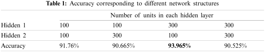
Figure 6: The optimal network structure diagram obtained by comparison

To observe the prediction effect of the model on the training data, 30 data points with fixed L2=0.2,L1∈(0.01,0.2) were randomly generated, and the Fig. 7 was obtained after eight predictions.

Figure 7: When L2 = 0.2, the number of minimum Gaussian quadrature points satisfying the given accuracy varies with L1

In Fig. 7, the horizontal axis represents the variation range of L1, and the vertical axis represents the number of Gaussian quadrature points corresponding to the change of L1. The blue thick solid line, marked as a star, represents the real number of Gaussian quadrature points (real label), and the other eight lines correspond to the results of eight predictions, respectively. As can be observed from Fig. 7, the number of Gaussian quadrature points increases with the increase of L1. The prediction results of the other eight lines are only inconsistent with the real value in the L1 range of 0.025 to 0.035, which accounts for 1/19 of the overall interval. Therefore, it has little influence on the prediction results and proves the effectiveness of the prediction model.

Similarly, 30 pieces of fixed data L1=0.05,L2∈(L1,0.5) are generated and randomly predicted eight times to obtain Fig. 8.

Figure 8: When L1 = 0.05, the number of minimum Gaussian quadrature points satisfying the given accuracy varies with L2

As shown in Fig. 8, the number of Gaussian quadrature points decreases with the increase of L2. Similar to Fig. 7, although the other eight lines do not coincide with the curves of real values, the overall trend is stable, which demonstrates that the model has good generalization ability. A small number of prediction errors occur in the range of L2 from 0.2 to 0.3 in Fig. 8, which reflects the inevitable randomness of the prediction.

4.3 The Time Required to Define the Optimal Model

Fig. 9 shows the CPU time required to determine the optimal model, which consists of the data preparation time in Section 4.1 and the model training and debugging time in Section 4.2. Define the total time as T, the data preparation time as T1, and the model training and debugging time as T2. Then T = T1 +T2. It can be seen that the time required to determine the optimal model increases linearly as the number of training data increases. In addition, the data preparation time is significantly greater than the training and debugging time of the model.

Figure 9: The CPU time required to determine the optimal model

5  Application of the Two-Dimensional Potential Problem

To verify the accuracy of the model, the two-dimensional potential problem of a circular structure discretized by equal length and unequal length are taken as examples. The specific process of the application is presented in Fig. 10.

Figure 10: Calculation steps in application phase

As shown in Fig. 10, the element information is stored in the input data. The lengths of L1 and L2 are calculated using the above-mentioned element information and determining whether L1 and L2 are consistent at this time with the feature range of the training data. Otherwise, the radius of the circle is adjusted. The calculated L1 and L2 are introduced into the optimal model as the test data to predict, and then the Gaussian quadrature points predicted previously are used to replace the Gaussian quadrature points in the traditional calculation to solve the Gaussian quadrature and subsequent equations. Finally, the numerical and analytical solutions on the boundary are calculated for comparison.

5.1 Discrete Circle Structure with Equal Length

As mentioned above, to control the feature parameters L1 and L2 within the feature range of the training data, the radius of the circle is set to 0.25, and the discrete circle structure with equal length is shown in Fig. 11.

In Fig. 11, the circle is discretized by 100 elements with equal length. Correspondingly, there are 100 collocation points (source points), located in the element center. Here, only the non-diagonal elements of the coefficient matrix are calculated; thus, a total of 9900 test data are obtained. The discrete element information is imported into the determined model as test data, and the comparison distribution between the predicted value and the real label is obtained, as presented in Table 2.

Figure 11: Discrete circle structure with equal length

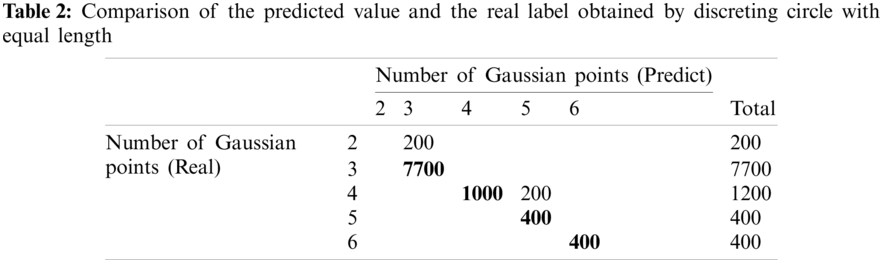
In Table 2, the number of coarsened data points on the diagonal represents the situation in which the real label and the predicted value are equal. There are 400 inaccurate data, as follows:

1.    The true value is 2, and the predicted value is 3 (200 copies).

2.    The true value is 4, and the predicted value is 5 (200 copies).

Therefore, the prediction accuracy of the model is 95.96%. Although a small amount of data is not predicted correctly, the predicted value is only slightly larger than the real label. Compared with the use of 15 Gaussian quadrature points, the calculation time of the Gaussian integral can be reduced while meeting the given precision. The effectiveness of the model prediction is verified.

It is known that the potential function satisfying the Laplace equation is

u1=x12−y12+2x1y1+3 (21)

It is assumed that the boundary condition u¯1 is prescribed, which can be obtained by substituting the discrete collocation point coordinates into Eq. (21). The analytical solution of the flux q¯1 at the collocation points are further calculated using Eq. (22):

q¯1=∂u1∂n=∂u1∂x1∂x1∂n+∂u1∂y1∂y1∂n=∂u1∂x1.cos⁡α+∂u1∂y1.cos⁡β=∂u1∂x1.x1r+∂u1∂y1.y1r (22)

where x1 and y1 denote the coordinates of the collocation point, and r denotes the radius of the circle.

It is worth noting that the numerical solution q1 of the boundary flux can be calculated by importing the predicted Gaussian quadrature points into the BEM code for computing. Finally, the numerical solution and the analytical solution of the flux are compared to obtain the relative error as presented in Table 3.

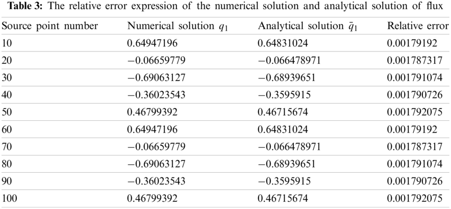
Here, 10 collocation points are selected on the boundary. As indicated in Table 3, the error between the numerical solution and the analytical solution of the flux at the collocation point is very small. Therefore, it is proved that the numerical solution obtained by using the minimum number of Gaussian quadrature points predicted by machine learning to perform Gaussian quadrature and the calculation of equations can almost replace the analytical solution. There is no need to use a sufficiently large number of the Gaussian quadrature points for calculation, which can not only reduce the calculation consumption of the Gaussian quadrature, but also achieve satisfactory accuracy.

5.2 Discrete Circle Structure with Unequal Length

Similarly, to control the feature parameters L1 and L2 within the feature range of the training data, a circle with radius of 0.25 is discretized with unequal length constant elements, and the discrete results obtained by making the center angle of the circle corresponding to each element within the range from 5∘ to 10∘ are shown in Fig. 12.

Figure 12: Discrete circle structure of unequal length

As depicted in Fig. 12, the circle is discretized into 47 elements and collocation points. Here, only the non-diagonal elements of the coefficient matrix are calculated, and thus a total of 2162 test data are obtained. The discrete parameter information of unequal length is imported into the determined model as test data, and the comparison of the distribution between the predicted value and the real label is made as presented in Table 4.

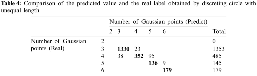
In Table 4, the number of coarsened data on the diagonal represents the situation in which the real label and the predicted value are equal. A total of 1997 data are predicted correctly; therefore the prediction accuracy of the model is 92.37%. Most of the 165 incorrectly predicted values are 1 larger than the real label, which is a similar result to that presented in Table 2. Using the minimum number of Gaussian quadrature points that meet the accuracy or a slightly larger value can significantly reduce the computational complexity of the Gaussian integral. Therefore, this model can be used to predict new data.

It is also known that the potential function satisfying the Laplace equation is:

u2=x22−y22+2x2y2+3 (23)

It is assumed that the boundary condition u¯2 is known, which can be obtained by substituting the discrete collocation point coordinates into Eq. (23). The analytical solution of flux q¯2 at the collocation poins are further calculated using Eq. (24):

q¯2=∂u2∂n=∂u2∂x2∂x2∂n+∂u2∂y2∂y2∂n=∂u2∂x2.cos⁡α+∂u2∂y2.cos⁡β=∂u2∂x2.x2r+∂u2∂y2.y2r (24)

where x2 and y2 denote the coordinates of the collocation point, and r denotes the radius of the circle.

In addition, numerical solution q2 can be obtained by importing the predicted number of Gaussian quadrature points into the BEM code for calculation. The relative error between the numerical solution and the analytical solution of the flux is compared as presented in Table 5.

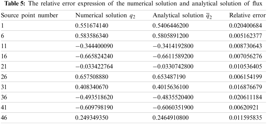
Similarly, as can be observed in Table 5, 10 collocation points are selected on the boundary. The error between the numerical solution and the analytical solution of the flux at the collocation point is very small, which verifies the effectiveness of the machine learning prediction. More importantly, it can provide an efficient reference for subsequent Gaussian integral calculations.

5.3 Time Comparison of Traditional BEM and Machine Learning Accelerated BEM

In addition to accuracy, efficiency is another important criterion for the proposed method. Here, the radius of the circle is changed so that the discrete feature parameters L1 and L2 are all within the feature range of the training data. Afterward, the minimum number of Gaussian quadrature points satisfying E1 can be predicted by transferring the feature parameters into the trained model.

It is worth noting that the number of Gaussian quadrature points only affects the calculation process of the coefficient matrix. Fig. 13 shows the time consumption of calculating the coefficient matrix by traditional BEM (Case 1) and machine learning accelerated BEM (Case 2) at different degrees of freedom. Among them, 15 Gaussian quadrature points are used in Case 1 to calculate the coefficient matrix, and the minimum number of Gaussian quadrature points obtained by machine learning prediction are used in Case 2 to calculate the coefficient matrix.

Figure 13: Time comparison of traditional BEM and machine learning accelerated BEM at different degrees of freedom

As can be seen from Fig. 13, the time consumption in Case 1 increases exponentially as the degrees of freedom increase, but the time increase in Case 2 is more moderate. It is worth noting that, once trained, the proposed model can perform the calculation of the coefficient matrix efficiently. What’s more, the computational efficiency of the proposed model may be even more prominent when the size of the data is larger.

6  Conclusion

In this paper, the multi-classification algorithm of a neural network is used to predict the minimum number of Gaussian quadrature points that meet the given precision in the Gaussian integral calculation of the BEM. The accuracy of the prediction can reach approximately 90%. Then, the predicted values obtained by the model are introduced into the BEM code to solve the numerical solution of the potential problem. After comparison with the analytical solution, it is found that the numerical solution can achieve high accuracy. More importantly, the use of predicted Gaussian quadrature points reduces the calculation time of the Gaussian integral to a certain extent, and also reduces the cost of the overall calculation of the BEM. Moreover, the high-order spline functions in the BEM further complicate this problem. Hence, the proposed technique is of great significance to guarantee the robustness, accuracy, and efficiency of BEM.

Funding Statement: The authors thank the financial support of National Natural Science Foundation of China (NSFC) under Grant (No. 11702238).

Conflicts of Interest: The authors declare that there are no conflicts of interest regarding the present study.

References

 1.  Akinyemi, L., Rezazadeh, H., Yao, S., Akbar, M. A., Khater, M. M. et al. (2021). Nonlinear dispersion in parabolic law medium and its optical solitons. Results in Physics, 26, 104411. DOI 10.1016/j.rinp.2021.104411. [Google Scholar] [CrossRef]

 2.  Ali Akbar, M., Akinyemi, L., Yao, S., Jhangeer, A., Rezazadeh, H. et al. (2021). Soliton solutions to the boussinesq equation through sine-gordon method and kudryashov method. Results in Physics, 25, 104228. DOI 10.1016/j.rinp.2021.104228. [Google Scholar] [CrossRef]

 3.  Hughes, T., Cottrell, J., Bazilevs, Y. (2005). Isogeometric analysis: CAD, finite elements, nurbs, exact geometry and mesh refinement. Computer Methods in Applied Mechanics and Engineering, 194(39), 4135–4195. DOI 10.1016/j.cma.2004.10.008. [Google Scholar] [CrossRef]

 4.  von Cottrell, J. A., Hughes, T. J. R., Bazilevs, Y. (2011). Isogeometric analysis: Toward integration of CAD and FEA. Bautechnik, 88(6), 423–423. DOI 10.1002/bate.201190060. [Google Scholar] [CrossRef]

 5.  Zheng, C. J., Chen, H. B., Gao, H. F., Du, L. (2015). Is the burton-miller formulation really free of fictitious eigenfrequencies? Engineering Analysis with Boundary Elements, 59, 43–51. DOI 10.1016/j.enganabound.2015.04.014. [Google Scholar] [CrossRef]

 6.  Zheng, C. J., Zhao, W. C., Gao, H. F., Du, L., Zhang, Y. B. et al. (2021). Sensitivity analysis of acoustic eigenfrequencies by using a boundary element method. The Journal of the Acoustical Society of America, 149(3), 2027–2039. DOI 10.1121/10.0003622. [Google Scholar] [CrossRef]

 7.  Chen, L., Lu, C., Zhao, W., Chen, H., Zheng, C. (2020). Subdivision surfaces-boundary element accelerated by fast multipole for the structural acoustic problem. Journal of Theoretical and Computational Acoustics, 28(2), 2050011. DOI 10.1142/S2591728520500115. [Google Scholar] [CrossRef]

 8.  Politis, C., Ginnis, A. I., Kaklis, P. D., Belibassakis, K., Feurer, C. (2009). An isogeometric bem for exterior potential-flow problems in the plane. SIAM/ACM Joint Conference on Geometric and Physical Modeling. New York, NY, USA: Association for Computing Machinery. DOI 10.1145/1629255.1629302. [Google Scholar] [CrossRef]

 9.  Scott, M. A., Simpson, R. N., Evans, J. A., Lipton, S., Bordas, S. P. A. et al. (2013). Isogeometric boundary element analysis using unstructured t-splines. Computer Methods in Applied Mechanics and Engineering, 254(2), 197–221. DOI 10.1016/j.cma.2012.11.001. [Google Scholar] [CrossRef]

10. Li, S., Trevelyan, J., Zhang, W., Wang, D. (2018). Accelerating isogeometric boundary element analysis for 3-dimensional elastostatics problems through black-box fast multipole method with proper generalized decomposition. International Journal for Numerical Methods in Engineering, 114(9), 975–998. DOI 10.1002/nme.5773. [Google Scholar] [CrossRef]

11. Nguyen, B. H., Tran, H. D., Anitescu, C., Zhuang, X., Rabczuk, T. (2016). An isogeometric symmetric galerkin boundary element method for two-dimensional crack problems. Computer Methods in Applied Mechanics and Engineering, 306(39–41), 252–275. DOI 10.1016/j.cma.2016.04.002. [Google Scholar] [CrossRef]

12. Peng, X., Atroshchenko, E., Kerfriden, P., Bordas, S. P. A. (2016). Linear elastic fracture simulation directly from cad: 2d nurbs-based implementation and role of tip enrichment. International Journal of Fracture, 204, 55–78. DOI 10.1007/s10704-016-0153-3. [Google Scholar] [CrossRef]

13. Peng, X., Atroshchenko, E., Kerfriden, P., Bordas, S. P. A. (2017). Isogeometric boundary element methods for three dimensional static fracture and fatigue crack growth. Computer Methods in Applied Mechanics and Engineering, 316, 151–185. DOI 10.1016/j.cma.2016.05.038. [Google Scholar] [CrossRef]

14. Chen, L., Wang, Z., Peng, X., Yang, J., Wu, P. et al. (2021). Modeling pressurized fracture propagation with the isogeometric bem. Geomechanics and Geophysics for Geo-Energy and Geo-Resources, 7, 51. DOI 10.1007/s40948-021-00248-3. [Google Scholar] [CrossRef]

15. Wang, Y., Xu, H., Pasini, D. (2017). Multiscale isogeometric topology optimization for lattice materials. Computer Methods in Applied Mechanics and Engineering, 316, 568–585. DOI 10.1016/j.cma.2016.08.015. [Google Scholar] [CrossRef]

16. Wang, Y., Wang, Z., Xia, Z., Poh, L. H. (2018). Structural design optimization using isogeometric analysis: A comprehensive review. Computer Modeling in Engineering & Sciences, 117(3), 455–507. DOI 10.31614/cmes. [Google Scholar] [CrossRef]

17. Lian, H., Kerfriden, P., Bordas, S. (2017). Shape optimization directly from cad: An isogeometric boundary element approach using t-splines. Computer Methods in Applied Mechanics and Engineering, 317, 1–41. DOI 10.1016/j.cma.2016.11.012. [Google Scholar] [CrossRef]

18. Chen, L., Lu, C., Lian, H., Liu, Z., Zhao, W. et al. (2020). Acoustic topology optimization of sound absorbing materials directly from subdivision surfaces with isogeometric boundary element methods. Computer Methods in Applied Mechanics and Engineering, 362, 112806. DOI 10.1016/j.cma.2019.112806. [Google Scholar] [CrossRef]

19. Simpson, R., Scott, M., Taus, M., Thomas, D., Lian, H. (2014). Acoustic isogeometric boundary element analysis. Computer Methods in Applied Mechanics and Engineering, 269, 265–290. DOI 10.1016/j.cma.2013.10.026. [Google Scholar] [CrossRef]

20. Keuchel, S., Hagelstein, N. C., Zaleski, O., Vonestorff, O. (2017). Evaluation of hypersingular and nearly singular integrals in the isogeometric boundary element method for acoustics. Computer Methods in Applied Mechanics and Engineering, 325, 488–504. DOI 10.1016/j.cma.2017.07.025. [Google Scholar] [CrossRef]

21. Chen, L., Marburg, S., Zhao, W., Liu, C. Chen, H. (2019). Implementation of isogeometric fast multipole boundary element methods for 2D half-space acoustic scattering problems with absorbing boundary condition. Journal of Theoretical and Computational Acoustics, 27(2), 1850024. DOI 10.1142/S259172851850024X. [Google Scholar] [CrossRef]

22. Chen, L., Lian, H., Liu, Z., Chen, H., Atroshchenko, E. et al. (2019). Structural shape optimization of three dimensional acoustic problems with isogeometric boundary element methods. Computer Methods in Applied Mechanics and Engineering, 355, 926–951. DOI 10.1016/j.cma.2019.06.012. [Google Scholar] [CrossRef]

23. Chen, L., Liu, C., Zhao, W., Liu, L. (2018). An isogeometric approach of two dimensional acoustic design sensitivity analysis and topology optimization analysis for absorbing material distribution. Computer Methods in Applied Mechanics and Engineering, 336, 507–532. DOI 10.1016/j.cma.2018.03.025. [Google Scholar] [CrossRef]

24. Chen, L., Zhang, Y., Lian, H., Atroshchenko, E., Ding, C. et al. (2020). Seamless integration of computer-aided geometric modeling and acoustic simulation: Isogeometric boundary element methods based on catmull-clark subdivision surfaces. Advances in Engineering Software, 149, 102879. DOI 10.1016/j.advengsoft.2020.102879. [Google Scholar] [CrossRef]

25. Chen, L., Chen, H., Zheng, C., Marburg, S. (2016). Structural-acoustic sensitivity analysis of radiated sound power using a finite element/discontinuous fast multipole boundary element scheme. International Journal for Numerical Methods in Fluids, 82(12), 858–878. DOI 10.1002/fld.4244. [Google Scholar] [CrossRef]

26. Yu, B., Cao, G., Huo, W., Zhou, H., Atroshchenko, E. (2021). Isogeometric dual reciprocity boundary element method for solving transient heat conduction problems with heat sources. Journal of Computational and Applied Mathematics, 385, 113197. DOI 10.1016/j.cam.2020.113197. [Google Scholar] [CrossRef]

27. Yu, B., Cao, G., Gong, Y., Ren, S., Dong, C. (2021). IG-DRBEM of three-dimensional transient heat conduction problems. Engineering Analysis with Boundary Elements, 128, 298–309. DOI 10.1016/j.enganabound.2021.04.014. [Google Scholar] [CrossRef]

28. Bradley, J. B. (1995). Neural networks: A comprehensive foundation. Information Processing and Management, 31(5), 786. DOI 10.1016/0306-4573(95)90003-9. [Google Scholar] [CrossRef]

29. Yagawa, G., Okuda, H. (1996). Neural networks in computational mechanics. Archives of Computational Methods in Engineering, 3(4), 435–512. DOI 10.1007/BF02818935. [Google Scholar] [CrossRef]

30. Oishi, A., Yoshimura, S. (2007). A new local contact search method using a multi-layer neural network. Computer Modeling in Engineering & Sciences, 21(2), 93–103. DOI 10.3970/cmes.2007.021.093. [Google Scholar] [CrossRef]

31. Lopez, R., Balsa-Canto, E., Oñate, E. (2008). Neural networks for variational problems in engineering. International Journal for Numerical Methods in Engineering, 75(11), 1341–1360. DOI 10.1002/nme.2304. [Google Scholar] [CrossRef]

32. Oishi, A., Yagawa, G. (2017). Computational mechanics enhanced by deep learning. Computer Methods in Applied Mechanics and Engineering, 327, 327–351. DOI 10.1016/j.cma.2017.08.040. [Google Scholar] [CrossRef]

33. Liang, L., Liu, M., Martin, C., Sun, W. (2018). A deep learning approach to estimate stress distribution: A fast and accurate surrogate of finite-element analysis. Journal of the Royal Society Interface, 15(138), 20170844. DOI 10.1098/rsif.2017.0844. [Google Scholar] [CrossRef]

34. Capuano, G., Rimoli, J. J. (2019). Smart finite elements: A novel machine learning application. Computer Methods in Applied Mechanics and Engineering, 345, 363–381. DOI 10.1016/j.cma.2018.10.046. [Google Scholar] [CrossRef]

35. Kirchdoerfer, T., Ortiz, M. (2016). Data-driven computational mechanics. Computer Methods in Applied Mechanics and Engineering, 304, 81–101. DOI 10.1016/j.cma.2016.02.001. [Google Scholar] [CrossRef]

36. Wang, Y., Liao, Z., Shi, S., Wang, Z., Poh, L. H. (2020). Data-driven structural design optimization for petal-shaped auxetics using isogeometric analysis. Computer Modeling in Engineering & Sciences, 122(2), 433–458. DOI 10.32604/cmes.2020.08680. [Google Scholar] [CrossRef]

This work is licensed under a Creative Commons Attribution 4.0 International License, which permits unrestricted use, distribution, and reproduction in any medium, provided the original work is properly cited.