Computer Modeling in Engineering & Sciences

DOI: 10.32604/cmes.2022.018286

ARTICLE

Study of Effect of Boundary Conditions on Patient-Specific Aortic Hemodynamics

Qingzhuo Chi1, Huimin Chen1, Shiqi Yang1, Lizhong Mu1,*, Changjin Ji2, Ying He1 and Yong Luan3

1Key Laboratory of Ocean Energy Utilization and Energy Conservation of Ministry of Education, Dalian University of Technology, Dalian, 116024, China
2School of Biomedical Engineering, Capital Medical University, Beijing, 100069, China
3Department of Anesthesiology, The First Affiliated Hospital of Dalian Medical University, Dalian, 116011, China
*Corresponding Author: Lizhong Mu. Email: muliz@dlut.edu.cn
Received: 13 July 2021; Accepted: 22 October 2021

1  Introduction

Aortic dissection (AD), caused by intimal splitting induced by pulsating blood, is one of the most complex cardiovascular diseases. The pathogenesis of AD is still unclear, but several associated conditions include hypertension and degeneration of the aortic media [1]. Degenerative diseases of the aortic media or rupture of the aortic intima causes damage, resulting in AD; then, blood passes through the tear into the aortic wall, and the aortic intima peels off [2]. The new passageway for blood inside the vascular media is called a false lumen.

Through computed tomography, three-dimensional reconstruction, and computational fluid dynamics (CFD) simulation, the blood flow behaviors and wall shear stress (WSS) of specific patients can be obtained. Moreover, tear locations can be predicted by the accurate estimation of WSS. High WSS or a high WSS gradient plays a role in vascular wall remodeling [3–6]. Research has reported that high WSS (10 to 30 Pa) can cause endothelial cells to express a unique transcriptional profile that may be useful in expansive arterial remodeling [7]. Some studies have found high WSS to correspond with extracellular matrix dysregulation and elastic fiber degeneration [3,4]. The expansive remodeling and degeneration of elastic fibers in the aorta may be related to AD occurrence. Cheng et al. [7] found high WSS distribution around a tear location, which may further expand the tear. Chi et al. [8] found that the entrance of type A dissection in three of five subjects was located at bifurcations on the aortic arch, where elevated WSS was also observed. Moreover, a higher branch angle may lead to higher WSS.

The boundary condition (BC) settings, including outflow and inflow conditions, for computational simulation are important for modeling the flow of the cardiovascular system. These settings are directly associated with the authenticity of CFD results, particularly the flow pattern and WSS distribution, and affect the reliability and comparability of the computational results. Liang et al. [9,10] reported that the inlet blood flow and waveform of the lesion considerably change the WSS and oscillatory shear index (OSI) in intracranial aneurysm. They also found that a change in the outflow distribution ratio in an aneurysmal artery causes significant changes in the flow field characteristics and WSS. Gallo et al. [11] compared different outflow BC strategies and indicated that the use of patient-specific BCs at the inlet and three branches outperformed other strategies, such as the use of a fixed outflow rate or partly patient-specific BCs. Chi et al. [8] observed the relationship between high WSS and tear locations on the aortic arch by using a fixed flow rate ratio among three outlets. However, the outlet BCs in the abovementioned works cannot reflect the Windkessel-based outlet BCs, which describe the pressure–flow relationship at each outlet. Pirola et al. [12] tested five sets of outlet BCs, namely a three-element Windkessel model (3-EWM), mass flow, waveforms, and 0-pressure, in an image-based model of a normal aorta. They found the physiological pressure waveforms and values were obtained by using a well-tuned 3-EWM at all outlets.

In addition, the valve, which is the only entrance for blood flow into the aorta, directly influences the flow field patterns of the ascending aorta (AAo), consistent with MRI-based inlet velocity profiles, [13,14] because of its large deformation during periodic opening and closing. Bonomi et al. [15] and Pasta et al. [16] reported that the aortic valve increased fluid dynamics abnormalities and therefore affected WSS distributions in the AAo. Moreover, a bicuspid aortic valve has been found to induce higher and asymmetric WSS, which may be related to changes in aortic morphology [17,18]. However, the valve, which is a complicated structure, is always simplified as a fixed diameter pillar [19] or completely neglected [12] because of its large deformation owing to fluid–structure interaction. It is vital to investigate how to combine the influences of inflow geometry on the hemodynamic behaviors of the AAo and aortic arch. The problem of physiological authenticity of the AAo in flow simulations can be better solved by considering the aortic sinus and auxiliary calculation domain. Although valves are still not considered in the current study, the auxiliary entrance and 3-EWM can significantly improve the physiology of the flow in the AAo and make the simulation results more valid than the results of previous studies [19–21].

In this study, two patient-specific models, namely, a type A dissection case and a normal aortic model, were used by reconstructing the computed tomography (CT) imaging data of the subjects. The effect of the flow BC on patient-specific aortic hemodynamics was investigated with or without the consideration of injection flow from the aortic valve, pressure control and 3-EWK model outlet conditions, and steady and unsteady inflow conditions.

2  Methods

2.1 Image Acquisition and Computational Modeling

This section presents detailed information on geometric reconstruction. The CT images used in this research had good resolution, with an in-plane resolution of 0.84 mm. The AAo and descending aorta (DAo) can be observed in Fig. 1a. Because an acute onset of AD is difficult to predict, only the CT dissection data of most of the patients were available. An imaging process may help us estimate the approximate geometry before tearing. The morphologic alteration of the aortic model is a long-term process [22], but the duration between the onset of type A AD and the capture of CT images is short; therefore, it was assumed that only limited morphology changes were captured before and after AD onset. Thus, the first CT data used for diagnosis were adopted to estimate and reconstruct the aorta before the dissection.

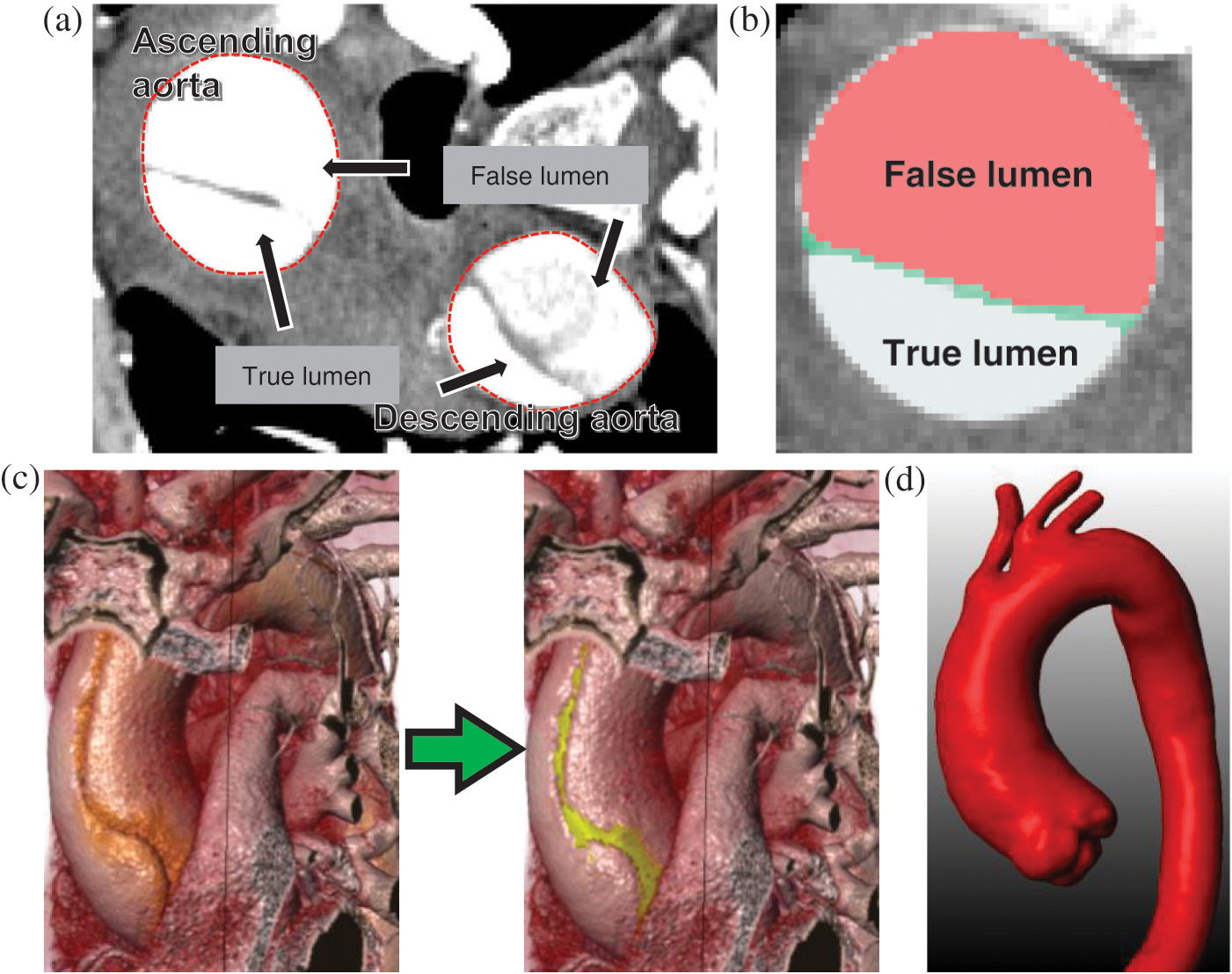
Figure 1: Main steps in patient-specific geometric reconstruction. (a) An axial CT image with the lumens and ascending and descending aorta. (b) Enlarged view showing the true lumen, false lumens, and the dissection. (c) AAo of a type A AD subject before and after estimation of the geometric model. (d) Model of the patient with type A AD after reconstruction and filtration

The “repairing” process of CT images of the tear features involved three steps. First, the areas of the true and false lumens and the gap between them were identified (Fig. 1b). Then, a Boolean sum of the lumens and gap was performed. When abnormal morphology was observed, further repairs were manually performed according to the shape of the true lumen and the spatial relationship of the neighboring slices. A reconstructed model before and after the repairing process is presented in Fig. 1c. Finally, a filtering operation was performed to smooth out the noise in the images (Fig. 1d).

The main aim of this study is to investigate the hemodynamics differences caused by the auxiliary structure at the aortic valve. In the computational domain, the proximal truncation began at two regions: the middle of the AAo and the aortic valve, and an auxiliary structure was established for models with the proximal truncation at the aortic valve [17,19].

The auxiliary field was created by “blending” the shape of a patient-specific aortic valve opening during peak systole with a circular face of 30 mm at a normal distance of 200 mm (Fig. 2a). The 200-mm distance enabled the full development of the flow injection. Moreover, the circular face prevented an alteration in flow rate when the shape of the aortic opening changed. The auxiliary domain was reoriented according to the outer contour of the aortic sinus and the proximal AAo. The distal truncated positions were selected at the brachiocephalic artery (BA), left common carotid artery (LCCA), left subclavian artery (LSA), and end of the DAo. Four auxiliary computational domains were separately established at the truncated sections of every outlet boundary.

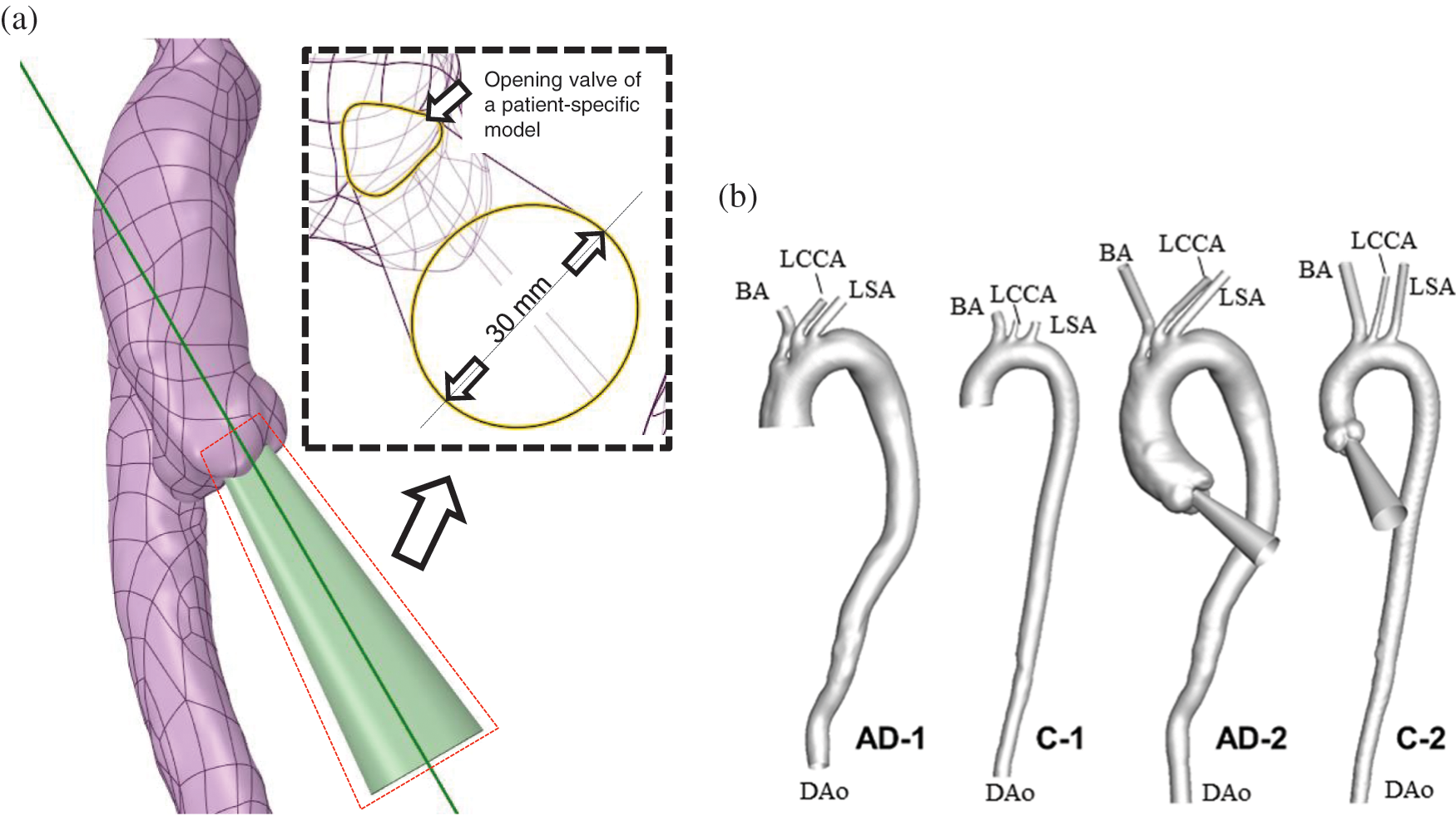
Figure 2: Design and establishment of the auxiliary entrance. (a) The layout of the AAo and auxiliary entrance, with the geometric details illustrated in the partially enlarged view. (b) AD and control subjects without and with the auxiliary computational domain

As depicted in Fig. 2b, the reconstructed AD subject and control subject for which the computational domain began at the middle of the AAo were named AD-1 and C-1, respectively. Meanwhile, the AD and control subject for which the computational domain began at the aortic valve were named AD-2 and C-2, respectively.

2.2 Computational Mesh Generation

The Fluent Meshing ver. 17.2 model and ICEM model were adopted for mesh generation. For AD-1 and C-1, a hexahedral O-grid was adopted because of its excellent performance and low computational cost. For AD-2 and C-2, a polyhedral mesh with 10 prismatic layers near the wall was generated to capture the geometric features around the aortic sinus (Fig. 3).

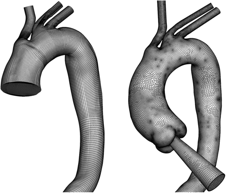
Figure 3: Overview of mesh generation in an aortic model within truncation and with an auxiliary entrance

All of the grids passed the mesh sensitivity test. Independent mesh experiments were conducted. A coarse hexahedral O-grid mesh and a corresponding fine mesh with 100% refinement, containing 251,264 and 809,417 cells, respectively, were tested. A relatively coarse polyhedral mesh with 700,000 polyhedral cells and a corresponding fine mesh with 100% refinement were tested. In the mesh sensitivity test, the relative changes in facet maximum WSS were less than 6% of the second-order truncation error. Moreover, according to the turbulence model, the Y+ values of all of the grids were less than 2. Considering the computational cost, a relatively coarse scheme was adopted.

2.3 Flow Model and BCs

The blood used in the simulation was treated as a Newtonian and incompressible fluid governed by the Navier–Stokes equations, which were solved using the finite volume method and spatially discretized using a second-order upwind scheme. The working fluid had the following physical parameters: viscosity of 4.0 m Pa⋅s and density of 1,060 kg/m3. The pressure velocity coupling was solved using the semi-implicit method for pressure-linked equations. The turbulence model, named shear stress transport (SST-Tran), was adopted in both steady- and unsteady-state simulations [23]. The SST-Tran can provide a reliable solution not only for the boundary layer but also the interior lumen [24]. The turbulence intensity was specified as 1.0% [24,25]. A rigid arterial wall with no-slip conditions was adopted, such that zero velocity was on the walls [26].

Table 1 presents the three sets of BCs at the model inlet and outlets, which consisted of the arch branches (BA, LCCA, LSA) and the aortic outlet located at the DAo (Fig. 4).

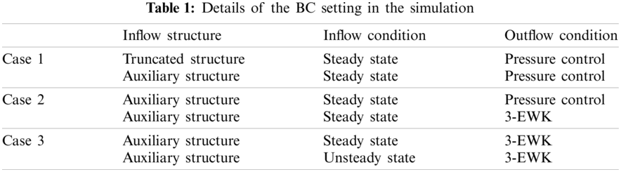
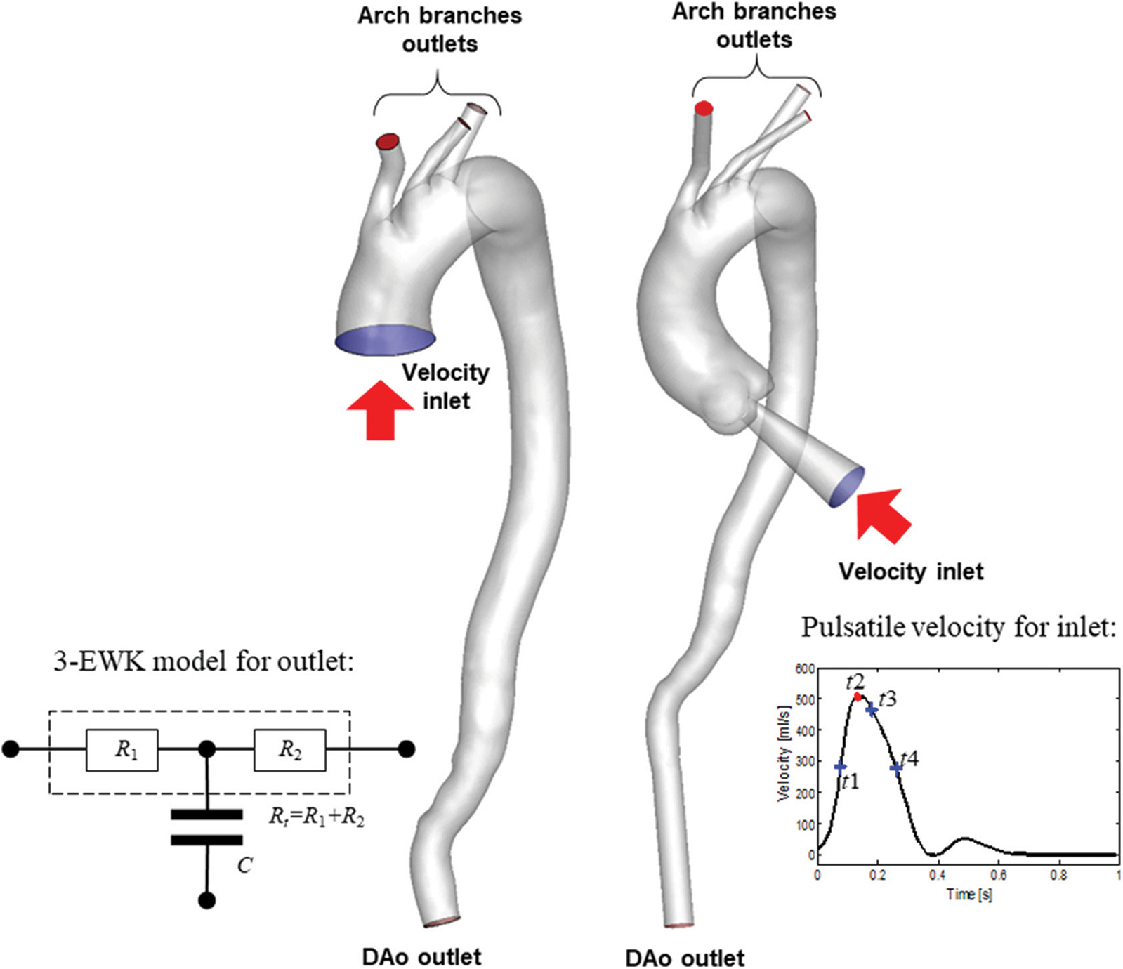
Figure 4: Schematic diagram and details of the BC setting

For the inflow condition, steady-state simulation was performed on all the aortic models, while unsteady-state simulation was performed only on models involving the aortic sinus. For models AD-1 and C-1, the constant (in-space) velocity was set as 0.2 m/s based on the literature [11], and the equivalent flow rate was 500 ml/s at the truncated section area. For models AD-2 and C-2, a flow rate of 500 ml/s was directly adopted [11]. During unsteady-state simulation, the pulsating inlet velocity user-defined function (UDF) was edited in ANSYS ver. 17.2 (Fig. 4 inset). Four key time points were considered, namely mid-acceleration (t1 = 80 ms), peak systole (t2 = 130 ms), mid-deceleration (t3 = 260 ms), and post-peak systole (180 ms). The post-peak systole corresponded to the maximum WSS distribution [23].

Meanwhile, the outlet conditions included pressure control and the 3-EWK parameters. The pressures assigned to the aortic branches were adjusted such that the total outflow rate of the aortic branches was 30%. The specific outflow rate of each bifurcation was related to its truncation area. A zero-pressure condition was assigned to the abdominal outlet.

The 3-EWK model provides a lumped parameter description of the vasculature located downstream of the outlet boundaries of the 3D domain. The model consists of a proximal (or characteristic) resistance (R1), compliance (C), and distal resistance (R2). These elements correspond to aggregate distal vascular properties, including viscous resistance, vessel wall distensibility, and blood inertia. The input impedance (Z) of the model can be expressed in the frequency domain as (ω)=R1+R2/1+jωCR2. Several studies support the parameter determination method in the 3-EWK model. The total resistance can be calculated as Rt=R1+R2 [27], where Rtcan be approximated as Rt=P¯/Q¯ according to previous research [28]; here, P¯ represents the mean pressure, which can be evaluated from available physiological blood pressure waveforms, and Q¯ is the mean flow rate of each outlet based on its area. The proximal resistance can be obtained as R1=ρC/A, where c is the pulse wave speed [29]. In summary, R2 can be calculated by subtracting R1 from Rt. The compliance element can be calculated as C=τ/Rt once Rtis determined using the equation above, where τ(=1.79 s) represents the time constant of the exponential fall-off of pressure during diastole [29]. Because of the similarity between the outflow boundary settings in this study and those of Kim et al. [30], the values of the Windkessel parameters can be calculated from the physiological data obtained via actual measurements in the work by Kim et al. [30] (Table 2). To make the 3-EWK model suitable for steady-state simulation, the relationship between the constant velocity (0.2 m/s) and time was given by the UDF.

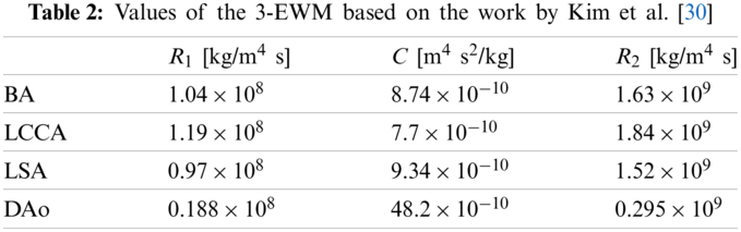
Fig. 5 illustrates the data transfer formula between the Fluent 3D domain and the 3-EWK model. The area-averaged volumetric flow Qn at the 3D domain boundary is computed and used in the 3-EWK model to derive the corresponding static pressure Pn at the boundary. The Windkessel model then transfers the pressure data Pn from the current time step to the 3D domain to calculate the flow values Qn+1 in the next iteration step. The initial condition for this process is the initial pressure Pn0at t=0.

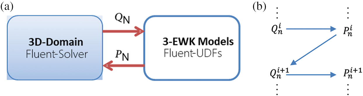
Figure 5: Coupling relationship between the fluent 3D domain and 3-EWK models (a); coupling boundary and scheme for the iterative update of pressure and flow (b)

Furthermore, in the unsteady-state simulations, seven cardiac cycles were needed to ensure the convergence of the pulsating pressure cycle. Convergence was reached when the residuals of both the mass and momentum conservation equations were less than 10−3. A second-order implicit time-stepping scheme was adopted with the fixed time-discrete scheme. The fixed time step was set less than or equal to 0.005 s, it did not depend on for the time step. The eighth cardiac cycle was prepared for the data extraction. Important hemodynamic parameters include WSS distribution, streamline, time-averaged WSS (TAWSS), and OSI contours [23].

The TAWSS on the vascular wall is quantified in a cardiac cycle by the flowing expression:

TAWSS=1T∫0T⁡|WSS(s,t)|dt

where T is a cardiac cycle period, and WSSis the transient WSS at position s.

The OSI, which measures the degree of change in WSS in a cardiac cycle, is expressed as

OSI=12[1−(|∫0T⁡WSS(s,t)dt|∫0T⁡|WSS(s,t)|dt)]

3  Computational Results and Discussion

3.1 Flow Characteristics Induced by Auxiliary Entrance

Fig. 6 shows the streamline and WSS distribution of the steady-state simulations of the AD and control samples. The WSS was normalized to highlight the effect of the auxiliary entrance on the WSS distribution, which is defined as the ratio of the local WSS to the maximum WSS of the aortic model. As depicted in Fig. 6, elevated WSS was observed at bifurcations of the BA and LCCA in all of the models. Moreover, subjects with an auxiliary entrance provided more information on the WSS distribution in the AAo. Higher WSS occurred in the outer curve of the AAo (Fig. 6, red arrow) but was absent in subjects without the auxiliary entrance structure. The WSS difference was reflected in the different flow patterns in the AAo. As depicted in the streamlines of the AD and control cases in Fig. 6, the helical flow pattern induced by the injection flow was related to the auxiliary entrance in the whole AAo model. In contrast, the AAo truncated in the middle exhibited almost-laminar flow. Moreover, the jet flow at the aortic valve accelerated the flow velocity, and high-speed flow was maintained until the flow approached the outer curve of the AAo, which increased the WSS distribution. Nevertheless, the flow pattern in the AD groups developed similarly in the distal sections of the DAo with or without an auxiliary entrance. The similar flow characteristic in AAo with an auxiliary entrance structure was observed in our in-vitro experiment of a simplified aorta [31].

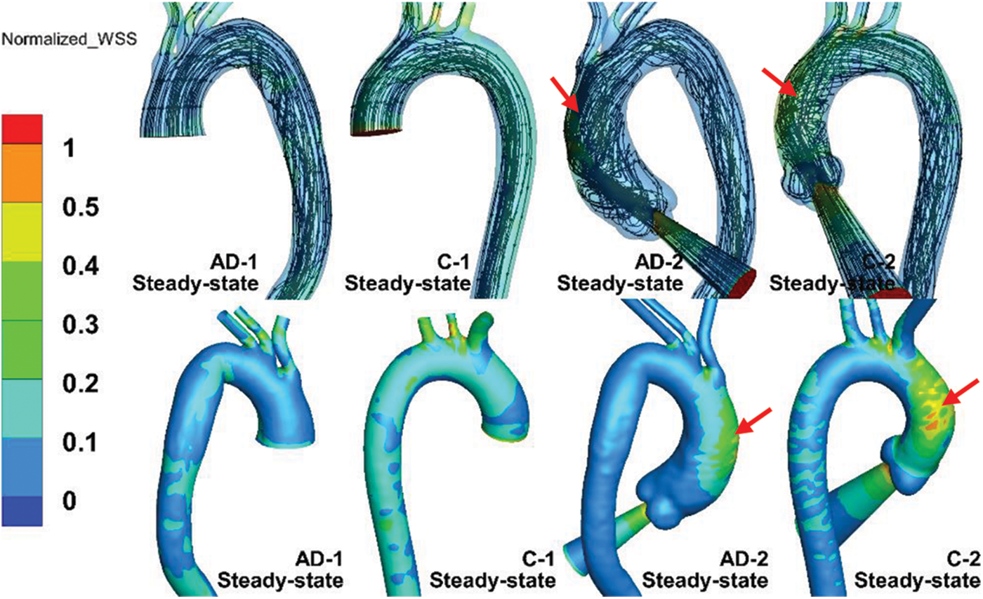
Figure 6: Streamline and normalized WSS in steady-state simulations of AD-1, C-1, AD-2, and C-2

However, compared with the results provided by four-dimensional magnetic resonance imaging (4D-MRI) [20], the helical flow inside the AAo, which essentially follows a physiological pattern, can hardly be simulated. A slice in the middle of the AAo is presented in Fig. 7. The slice location was based on a 4D-MRI study by Miyazaki et al. [32] For both the AD and control cases, the overall view depicts the slice location in the figure. Meanwhile, the velocity of all of the subjects was normalized. Fig. 7 depicts an in-plane image of the same AAo location in the control and AD models, with or without auxiliary entrance. The models without auxiliary entrance mainly exhibited laminar flow, whereas those with auxiliary entrance exhibited helical flow, consistent with the 4D-MRI results of AAo [14,32]. The findings indicate that the flow field results of the geometric AD-2 and C-2 with auxiliary entrance were closer to physiological reality. Thus, the physiological authenticity of the AAo in flow simulations can be improved by considering the aortic sinus and auxiliary calculation domain.

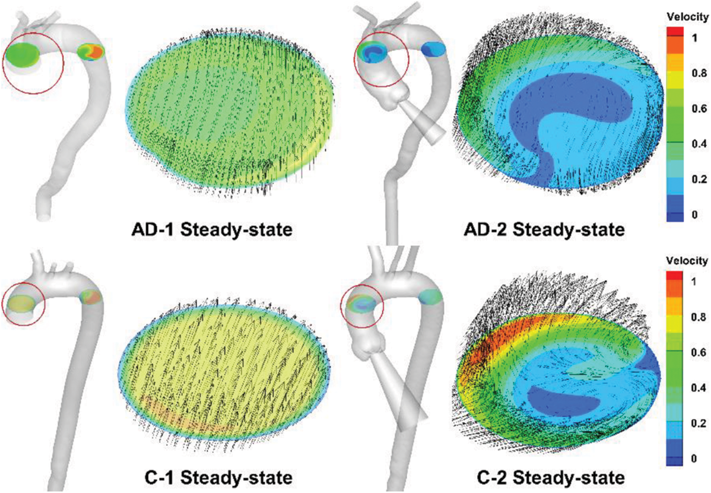
Figure 7: Steady-state simulation results for AAo, with the slice location indicated by the red circle and corresponding enlarged sections

3.2 Hemodynamic Difference Related to Outflow and Inflow Conditions

According to the results in Fig. 7, the hemodynamics of the aortic model does not depend considerably on the valve inlet structure. The hemodynamics of the aortic model with an auxiliary entrance structure approximated the physiological state. To compare the effects of the BC settings of Case 2 and Case 3 (Table 1) on their hemodynamics, the aortic model with an auxiliary entrance was adopted in the following simulations.

Fig. 8 compares the streamline and normalized TAWSS distribution in the aortic model with the BC setting of Case 2. As the black circle indicates, the AD sample and healthy aortic model exhibited highly similar WSS distributions in the AAo. Owing to the jet inflow, high WSS was concentrated at the AAo segment, which can be observed in the streamline results (red arrows). One marked difference of the normalized WSS is the high-WSS area in the AAo with the 3-EWK outflow conditions, as shown by the red arrows. Moreover, the aortic branches exhibited high WSS. The aortic branches with the 3-EWK outflow conditions showed a much larger high-WSS area (white arrows).

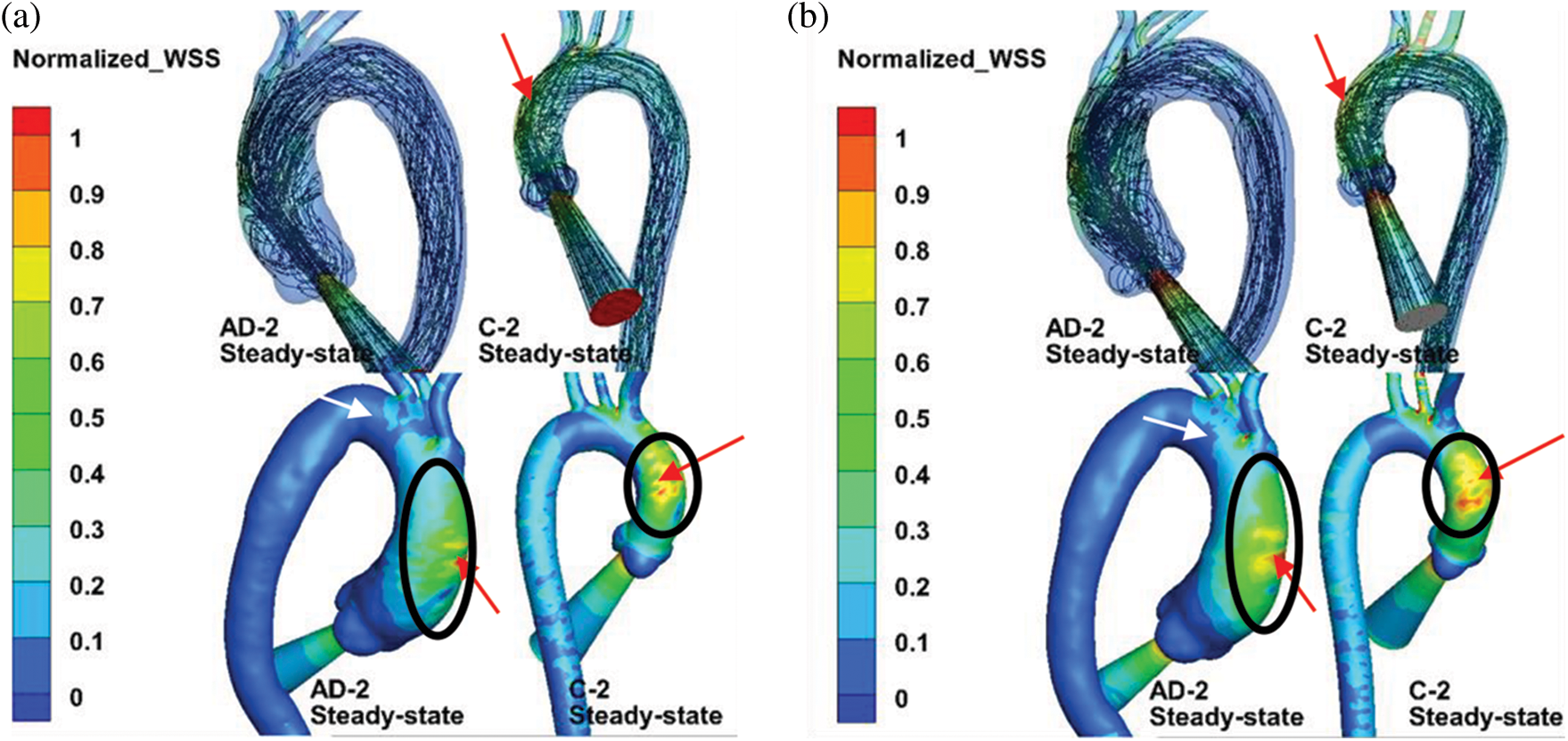
Figure 8: (a) Comparison of streamlines and normalized WSS under the steady inflow state with pressure control. (b) 3-EWK model outlet conditions

Fig. 9 compares the numerical results of the steady- and unsteady-state solutions, where the upper and lower panels in the figure are the streamlines and normalized TAWSS results within the inlet BC. The streamlines of the unsteady-state solution in AD-2 and C-2 are the numerical results corresponding to 180 ms (post-peak systole). The definition of normalized TAWSS is the same as that of the normalized WSS.

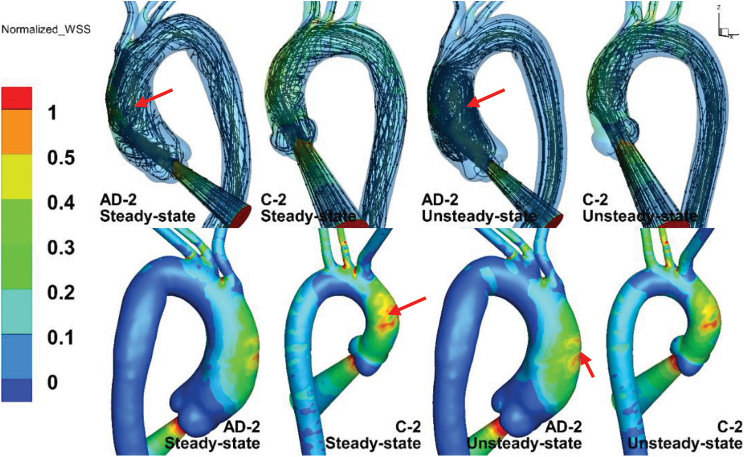
Figure 9: The streamlines (upper panels) and normalized TAWSS (lower panels) results within the inlet BC at steady state and unsteady state

The TAWSS distributions in the AAo, aortic arch, and DAo under steady state were similar to those under unsteady state. As shown by the red arrows, the maximum TAWSS in the C-2 case under steady state was slightly larger than that under unsteady state, while the TAWSS in AD-2 under unsteady state was much larger. The streamline of C-2 under steady state shared many similarities with that under unsteady state in a helical flow pattern. However, the streamline of AD-2, in which the AAo could be considered dilated, exhibited a more intense vortex pattern under unsteady state than under steady state, as indicated by the red arrows in the upper panels of Fig. 9. The streamlines of AD-2 under unsteady state indicates potentially more complicated flow patterns when the aorta becomes dilated.

Although the steady-state results display comparable streamlines and TAWSS distributions with those under unsteady state at a specific moment, unsteady-state simulation can provide additional details of hemodynamics parameters. Fig. 10 provides a group of unsteady-state results for different moments. The legend of the WSS color map was re-edited according to the biomechanical significance of the WSS level to endothelial cells. The WSS level values were chosen as 0.4, 1.5 to 2.5, 10 to 30, and >30 Pa. At t = 80 ms (mid-acceleration), the flow pattern was helical in AD-2 but laminar in C-2. Because of the AAo dilation, the AAo exhibited lower WSS distribution under a uniform inflow rate. However, the WSS on aortic bifurcations was still elevated. At peak systole, flow injection reached the outer curve at the root of the AAo (Fig. 10b). Then, the injection-induced flow pattern gradually developed in the post-peak systole (Fig. 10c). Vortex and helical flow occurred from the post-peak systole to mid-deceleration (Figs. 10c and 10d), which has been verified through 4D-MRI observations [20,32]. The vortex pattern resulted in OSI distribution throughout the AAo. The root of the AAo, proximal region of the BA ostia, and inner curve of the aortic arch exhibited high OSI.

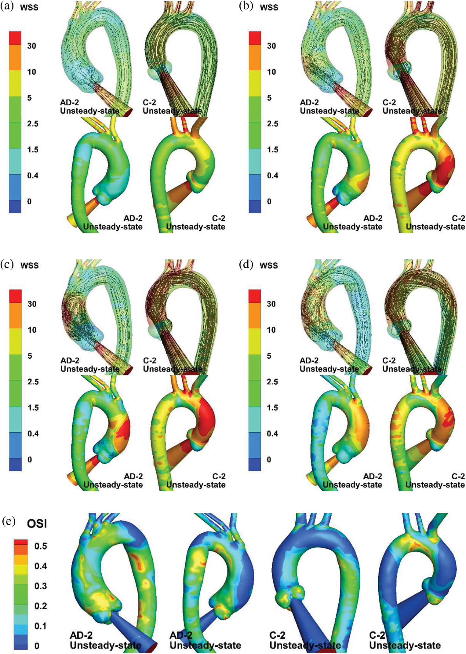
Figure 10: Numerical results of unsteady-state simulation. (a–d) Streamlines and WSS of AAo and aortic arch at t = 80 (mid-acceleration), 130 (peak systole), 180 (post-peak systole), and 260 ms (mid-deceleration). (e) OSI distribution of AD-2 and C-2

4  Discussion

Cardiovascular CFD can provide patient-specific aortic models to assist physicians in noninvasive AD diagnosis and can predict the hemodynamic characteristics of the aorta after AD surgery. It has been reported that changes in the aortic hemodynamic parameters, such as the WSS gradient and OSI, are associated with tear occurrence and AD development. Chi et al. [8] found that an abnormal WSS concentration on the aortic arch was closely related to the tear location in an AD model. Ensuring the accuracy of numerical calculation results is vital for making critical decisions regarding diagnosis [33], surgical planning [34], and medical device designs [35].

However, owing to the difficulty of the in vivo measurement of flow and pressure in patients, the accurate information required for CFD is often lacking. A reasonable BC setting is important to improve the calculation reality and approximate patients’ physiological state. In this study, the introduction of an auxiliary entrance structure made the numerical results closer to the physiological state and effectively improved the numerical authenticity, as the results were close to published 4D-MRI results [20,32]. The helical flow inside the AAo was reproduced. The high shear stress distribution on the AAo wall, caused by pulsating jet flow through the aortic valve, was well simulated. The introduction of the auxiliary entrance structure is a simple and effective approach to optimize the AAo hemodynamic characteristics. It not only simplifies the aortic valve structure but also considers the effect of jet flow. Therefore, it can make the evaluation of the changes in aortic hemodynamic parameters more accurate and contribute to the prediction of aortic laceration.

Furthermore, several studies have adopted the 3-EWK parameters for the outflow conditions [12,20,36], considering the proximal and distal resistances and compliance. The model can be useful for evaluating the hemodynamics performance of surgical or interventional procedures with unclear postoperative pressure or flow [37]. According to the results of Pirola et al. [12], the outflow BCs greatly influence the hemodynamic characteristics of the aorta. However, if an auxiliary jet entrance structure is adopted, the influence of the outlet boundary, such as the pressure flow boundary and 3-EWK model boundary, seems negligible. In the current study based on the 3-EWK model, there was no considerable difference in the flow pattern at peak systole and TAWSS distribution between the steady-state and unsteady-state results. This means that with the adoption of the 3-EWK model, more accurate simulation results of the aorta can be obtained under steady flow at peak systole, indicating that for the analysis of aortic blood flow dynamics, the inflow structure may play a more crucial role than the outlet BCs.

However, this study has some limitations. The values of the 3-EWK model were based on the literature [27–29]. It has been reported that the 3-EWK model parameter values affect the numerical simulation results [20]. Patient-specific values of the 3-EWK model will be considered in further research. Second, the WSS and pressure drop in the rigid aorta case with vascular wall compliance may be different from that without vascular wall compliance [37]. Vascular wall compliance and pulsatile blood flow can lead to oscillations in the wall displacement, as reported by Mu et al. [38]. Moreover, fluid–structure interaction can result in low oscillatory shear stress distribution. Furthermore, the current work still lacks experimental verification of the results of different flow patterns in the AAo. In the next study, an in vitro experiment based on a silicone aortic model will be performed to investigate the influence of wall compliance on fluid patterns in the AAo.

5  Conclusions

In this study, we compared the changes in hemodynamic parameters in a type A dissection model and normal aortic model under different BCs: inflow from the aortic valve, pressure control and 3-EWK outflow conditions, and steady and unsteady inflow conditions. The auxiliary entrance structure remarkably enhanced the physiological authenticity of numerical studies of flow in the AAo. The steady-state and unsteady-state simulations of the aortic model with auxiliary entrance exhibited highly similar TAWSS distributions at the AAo wall and aortic arch branches. Moreover, the pressure and 3-EWK model outlet conditions had little effect on the numerical results, indicating that the inflow structure plays a crucial role in hemodynamic simulations. With reasonable BC settings, such as the combination of the auxiliary entrance and the 3-EWM at all of the outlets, it could enhance the calculated hemodynamic parameters prediction (WSS, OSI, etc.) of the aorta close to its physiological authenticity, which is much more important for CFD based researches on aortic hemodynamic analysis, such as, the influence of aortic morphology (elongation accompanied by dilation of the ascending aorta [23], varied aortic tortuosity [39], etc.) on its hemodynamic characteristics, the prediction of occurrence of aortic dissection via abnormal WSS distribution or OSI positions, as well as AD diagnosis and evaluation of surgical strategy of aortic dissection surgery by comparing the changes of hemodynamic parameters.

Funding Statement: This work was partially supported by the National Natural Science Foundation of China [No. 51976026] and the Fundamental Research Funds for the Central Universities [DUT21JC25, DUT20GJ203].

Conflicts of Interest: The authors declare that they have no conflicts of interest to report regarding the present study.

This work is licensed under a Creative Commons Attribution 4.0 International License, which permits unrestricted use, distribution, and reproduction in any medium, provided the original work is properly cited.