| Computer Modeling in Engineering & Sciences |
DOI: 10.32604/cmes.2022.017532
ARTICLE
Parameter Estimation Based on Censored Data under Partially Accelerated Life Testing for Hybrid Systems due to Unknown Failure Causes
Department of Basic Sciences, College of Science and Theoretical Studies, Saudi Electronic University, Dammam, 32256, Saudi Arabia
*Corresponding Author: Mustafa Kamal. Email: m.kamal@seu.edu.sa; kamal19252003@gmail.com
Received: 18 May 2021; Accepted: 11 October 2021
Abstract: In general, simple subsystems like series or parallel are integrated to produce a complex hybrid system. The reliability of a system is determined by the reliability of its constituent components. It is often extremely difficult or impossible to get specific information about the component that caused the system to fail. Unknown failure causes are instances in which the actual cause of system failure is unknown. On the other side, thanks to current advanced technology based on computers, automation, and simulation, products have become incredibly dependable and trustworthy, and as a result, obtaining failure data for testing such exceptionally reliable items have become a very costly and time-consuming procedure. Therefore, because of its capacity to produce rapid and adequate failure data in a short period of time, accelerated life testing (ALT) is the most utilized approach in the field of product reliability and life testing. Based on progressively hybrid censored (PrHC) data from a three-component parallel series hybrid system that failed to owe to unknown causes, this paper investigates a challenging problem of parameter estimation and reliability assessment under a step stress partially accelerated life-test (SSPALT). Failures of components are considered to follow a power linear hazard rate (PLHR), which can be used when the failure rate displays linear, decreasing, increasing or bathtub failure patterns. The Tempered random variable (TRV) model is considered to reflect the effect of the high stress level used to induce early failure data. The maximum likelihood estimation (MLE) approach is used to estimate the parameters of the PLHR distribution and the acceleration factor. A variance covariance matrix (VCM) is then obtained to construct the approximate confidence intervals (ACIs). In addition, studentized bootstrap confidence intervals (ST-B CIs) are also constructed and compared with ACIs in terms of their respective interval lengths (ILs). Moreover, a simulation study is conducted to demonstrate the performance of the estimation procedures and the methodology discussed in this paper. Finally, real failure data from the air conditioning systems of an airplane is used to illustrate further the performance of the suggested estimation technique.
Keywords: Step stress partially accelerated life test; progressive hybrid censoring; data masking; power linear hazard rate distribution; hybrid system
Computers, cellphones, and many other systems of competitive innovation and modernization are getting increasingly complex, with numerous subsystems and sub-assemblies in each. Furthermore, these subsystems and subassemblies are made up of several components, making the life testing procedure for such systems more complicated. The study of reliability and life testing of systems, subsystems, or components is entirely depend on lifetime data, which is a combination of two important pieces of information. The first is to determine the product’s failure time, and the second is to determine the reasons for its failure. The failure times of the system can easily be recorded, but the cause of the failure is not always recognized due to a variety of factors, including a lack of adequate diagnosis, time and expense constraints for comprehensive failure analysis, and numerous component failures with destructive consequences. As a result, in the literature of reliability and life testing analysis, such data in which the true cause of system failure is unknown and only a minimum random subset of the reasons that are responsible for system failure can be recognized is referred to as masked data. See [1,2] for more details.
The overall quality of today’s products due to the existing advanced technology based on computers, automation and simulation has been improved drastically, which makes them extremely reliable and trustworthy. Consequently, gathering failure data for testing of such extremely reliable products using ordinary reliability tests (ORTs) has become a very costly and time-consuming process, making the use of ORTs impractical. Hence, ALTs are a more advanced approach for obtaining fast failure data by testing items under higher stress than normal, and then, a life stress relationship is used to get the product’s life characteristics under normal usage settings. According to [3], stress loading in ALT may be performed in a variety of ways, although the most commonly used stress loadings are constant, step, and progressive stress loadings. Many scholars so far have looked at the ALT models, including [4–10]. Assuming a lognormal lifetime distribution, Li et al. [5] proposed two types of Bayesian accelerated acceptance sampling plans for illustrating product reliability based on the product’s operating characteristic curve under Type-I censoring. The first plan addresses both producer and customer risks at the same time, whereas the second exclusively considers consumer risk. Rahman et al. [9] used MLE methods for estimating the parameters of Burr-X life distribution parameters assuming that failure under arithmetically increasing stress levels of CSALT forms a geometric process. Ma et al. [10] proposed an optimum hybrid accelerated test plan under many experimental design restrictions by combining ALT with accelerated degradation testing and modeling the degradation process with an inverse Gaussian process.
However, there are situations when these sorts of relationships are not possible. Because of the prevalence of this issue in ALTs, PALTs are considered to be preferable option and are usually implemented in two ways. The first is constant stress PALT, while the second is SSPALT. In SSPALT, a sample of components or systems is first tested under normal usage circumstances for a certain amount of time, and then systems or components that have not failed are allocated to testing at accelerated conditions until all items fail or a predetermined censorship scheme is met. SSPALT analysis has been considered by many authors since it was first suggested by [11,12] as a TRV model. Bhattacharyya et al. [13] developed a tampered failure rate model using the TRV model. Bai et al. [14–16] are others who considered SSPALT using the same concept of the TRV model for different distributions and censoring schemes. Assuming the TRV model, Zhang et al. [17] discussed the MLEs of the unknown parameters for the extended Weibull distribution. Ismail et al. [18,19] investigated the MLEs of the parameters of the Weibull and Burr Type-XII distributions, respectively, and compared the results based on two different PrHC schemes. Mahmoud et al. [20–22] deals with SSPALT based on an adaptive type PrHC scheme to obtain estimates of parameters using MLEs and Bayesian estimates (BEs) of generalized Pareto, two-parameter exponentiated Weibull and Lindley distributions, respectively.
A considerable number of studies have been carried out on parameter estimation using mask data based on ORTs since it was first introduced by [1,2]. Considering different failure distributions, Guess et al. [23–33] utilizes the MLE technique for estimating model parameters for a single component or a series or parallel systems of two or three components, whereas Reiser et al. [34–43] considered BE technique based on different priors. As it was discussed earlier, many real-life systems or machines these days are made of hybrid structures which are a combination of series and parallel subsystems. More complex systems can have many hybrid subsystems which are generally connected in parallel-series, series-parallel, series-parallel-series, and parallel-series-parallel configurations and so on. Peng et al. [44] developed a Bayesian approach for system reliability evaluation and prediction in which pass-fail data, lifespan data, and deterioration data are integrated coherently at multiple system levels. Yang et al. [45] developed an Adaptive Bayesian Melding reliability evaluation technique for analyzing and assessing the reliability of a hierarchical system with imperfect prior knowledge. They also expanded the concept to a broader multi-level hierarchical structure by employing a more effective method of pooling inconsistent priors. Yang et al. [46] proposed a Bayesian reliability approach for complex systems with dependent life metrics and developed a likelihood decomposition method to convert the overall likelihood into a product of explicit and implicit evidence-based likelihood functions. As of now, only a limited number of research papers considering hybrid systems based on ORTs have been published. Considering three component parallel-series and series-parallel systems, Wang et al. [47] obtained the MLEs of the parameters based on masked data assuming constant and linear hazard rate of independent components. Sha et al. [48] considered a hybrid system of three dependent components and obtained the MLEs based on mask data assuming a bivariate exponential distribution. Cai et al. [49] considered the same system as in [48] and derived the MLEs based copula function under mask cause of failure. Recently, Rodrigues et al. [50,51] used more complex structures based on four or five components and obtained MLEs and BEs under incomplete data.
Only a few studies on ALTs so far that focused on hybrid systems and masked data have been published in available research. Reference [52] under SSALT, describes the procedure of obtaining MLEs of the parameters of the Weibull distribution for a series system based on an expectation minimization algorithm assuming symmetric masking. Considering masked interval data in SSALT, Fan et al. [53] obtained estimates of the parameters of the exponential distribution. Xu et al. [54,55] described the general Bayesian analysis of the series system masked failure data for the log-location-scale and Weibull distributions respectively under SSALT. Assuming the same exponential hazard rate for a four components hybrid system, Shi et al. [56,57] obtained the MLEs of unknown parameters of the model based on the masked data under SSPALT and CSPALT respectively. Shi et al. [58] considered two different hybrid systems of three components and then obtained MLEs of the modified Weibull distribution.
To the best of our knowledge so far, no article has been published that considers SSALT for PLHR distribution for a hybrid system under masked data. Much of the sources listed above considered hazard rates that are monotonic in nature, but there are cases where the hazard rate is not monotonic. The primary goal of this work is to describe the SSPALT using a more flexible PLHR that can be used when failure rates indicate non-monotonic characteristics for hybrid systems. To illustrate the considered estimation procedure under SSPALT using PrHC masked data, a three-component hybrid system is considered. The rest of the paper is organized as follows, Section 2 addresses the formulation of the SSPALT model for PrHC masked data from a hybrid system and some useful assumptions. The MLEs and corresponding ACIs and ST-B CIs of the parameters and acceleration factor are discussed in Section 3. In Section 4, we conducted a simulation study to demonstrate the performance of the estimation procedures and the methodology discussed in this paper. Section 5 addresses the suggested approach’s real-life data applicability. Finally, we conclude our study in Section 6.
2 Design and Assumptions of the Model
In reliability and life testing experiments/studies, hazard rate is the most important function since it plays a very important role in characterizing the aging process of the systems and hence in classifying failure time distributions, more details can be seen in [59]. Commonly used hazard rates are constant, linear and power hazard rates. However, distributions derived from these hazard rates are very useful and popular in reliability and life testing theory when the failure rate depicts monotonic properties, but they cannot be used to fit non-monotonic failure rates. Therefore, in this paper, a more flexible PLHR distribution introduced by [60] that is derived from the combination of linear and power hazard rates is considered. Different shapes of hazard rate and density function of PLHR distribution with different values of parameters are given in Figs. 1 and 2, respectively. The Probability density function (PDF), cumulative distribution function (CDF), reliability function (RF) and the hazard rate (HR) of PLHR distribution are given respectively by the following equations:
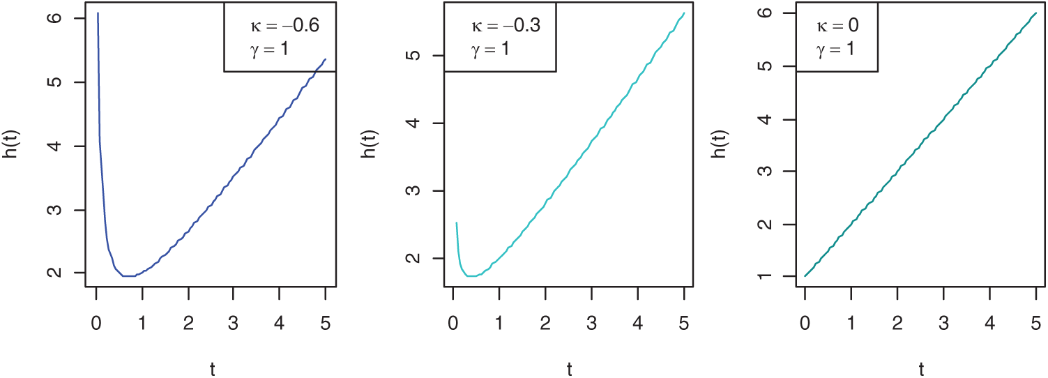
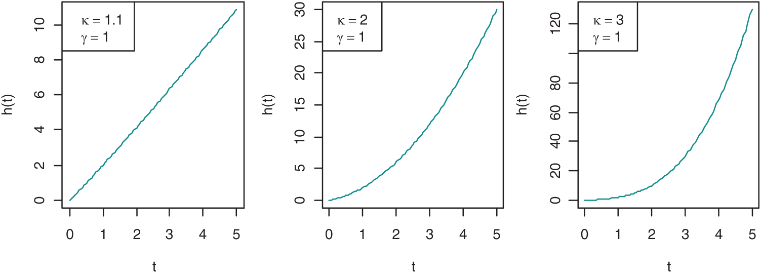
Figure 1: Shapes of the HR function of PLHR distribution with different values of the parameters
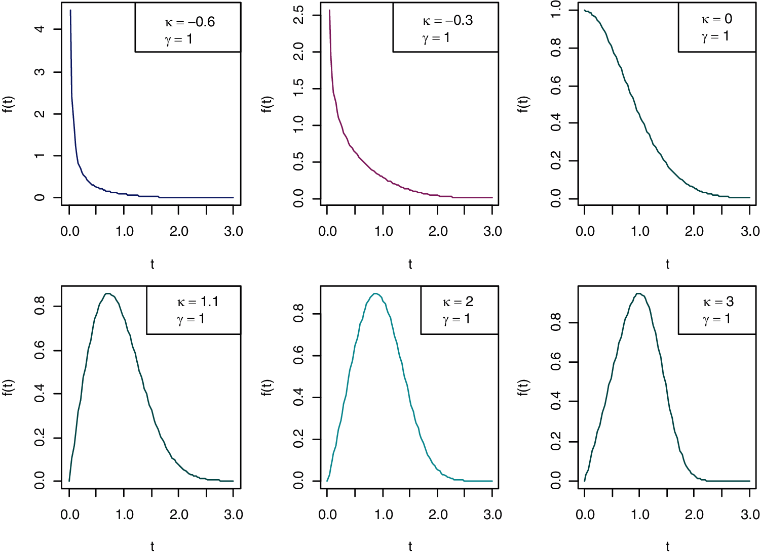
Figure 2: Shapes of the PDF of PLHR distribution using different values of the parameters
In this paper, the following assumptions are made in order to describe the SSPALT model for a hybrid structure under PrHC masked data:
1.
2. The system under consideration is a series parallel system containing three independent components j = 1, 2, 3 which is described by Fig. 3 as follows:
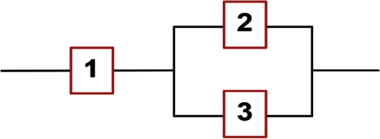
Figure 3: A series parallel hybrid system of three components
3. The lifetime
4. The data masking mechanism is statistically independent of the various stress conditions used in the experiment and the actual cause of failure of the system.
5. The lifetime of jth component at normal stress
6. Let the total lifetime T of a component in hybrid system under SSPALT is explained by TRV model and can be written as follows:
where X represents lifetime of the component at
Definition 2.1: Masking Probability
Suppose there are n system that are tested in the experiment and
Now, using the Assumption 4, above expression for masking probability can be written as follows:
2.3 Formulation of the SSPALT with PrHC Mask Data
PrHC scheme was first proposed and applied by [61] in traditional life tests. In SSPALT, suppose experiment is first started by randomly choosing n similar systems of three components described in the Fig. 3 to be assigned to test at the normal stress level
Now, using Eqs. (10), (12) and the PrHC masked data given in Eq. (16), we can write the likelihood function for the hybrid system under SSPALT as follows:
where,
Theorem 2.1: For a hybrid system consist of j independent components described in Fig. 3 having lifetime
Proof:
Probability that the system i is failed due to component j under mask occurrence
Now, the lifetime
And, therefore the RF of the system i can be obtained as follows:
Similarly, the probability densities of hybrid system i which is failed due to component j at time
For simplifying notations, let denote
Now using Eqs. (11), (15), (17) and Assumption 4, we obtained following:
which completes the proof.
Applying Eqs. (11), (14) and (16) in Eq. (13), we obtained the following form of the likelihood function [56]:
where, at use stress level
similarly, at accelerated stress level
3 Estimation of Model Parameters
To obtain the estimates of parameters, the MLE technique is used. Now, taking log on both sides of Eq. (18) and making some adjustments, the log likelihood function (or Score function)
where, we assume
Now, differentiating Eq. (19) partially with respect to model parameter
The MLEs
One of the best redeeming features of MLE is due to its large sample properties. For large sets of data, the distribution of MLEs of the parameters is approximately normal. As it is discussed in the last subsection, the likelihood equations for finding MLEs are virtually impossible to solve in close form and, hence the exact distribution of the MLEs is nearly impossible to find for a complex situation such as the one we are dealing with. Therefore, we utilized the asymptotic properties of MLEs to construct the ACIs. The distribution of MLEs
where,
where the elements of F are given in Appendix A. Now
where,
This subsection deals with the bootstrap re-sampling approach for constructing parameters CIs in which the original data is assumed to be a population and then several samples are generated using the original data to create the CIs, for more details see [64–66]. We use the following algorithm to construct ST-B CIs [56]:
1. Find the MLEs
2. Now using MLEs
3. Using bootstrap sample obtained in Step 2, find estimate
4. Repeat above 3 steps
5. Compute
Here in this section of the paper, we are going to perform a simulation study to investigate and compare the performance of estimates for the hybrid system under SSPALT for PrHC masked data by utilizing the Monte Carlo simulation technique. The performance of MLEs assessed with their respective mean square errors (MSEs) and relative absolute biases (RABs). 95% ACIs are also constructed and their performance is investigated in terms of their respective ILs. First, we generated the hybrid progressive censored data from the considered distribution under SSPALT following some of the steps given in [58,64,67] and the complete steps of the algorithm are given as:
1. Specify the values of
2. To obtain a random censored sample of size r, first generate a random sample of size r from uniform distribution U(0, 1), suppose these generated samples are
3. Specify,
4. Define
5. Set
6. Similarly, find a sample at accelerated condition for fixed values of parameters
7. Following above steps, we generated the desired PrHC masked data from PLHR distribution in the form of Eq. (12).
8. Now, using the data obtained in Step 7, compute MLEs
9. Replicate Steps 2–9, 10,000 times, and obtain average MLEs, MSEs and RABs of the parameters.
10. Compute the 95% ACIs for the parameters of PLHR distribution and acceleration factor.
11. For different values of
In our study, we used four different censoring schemes generated from six different combinations of n and m with different fixed values of
Fig. 4 presents the plots of simulated samples and the histograms of the parameters to verify the convergence of the parameters. For this demonstration, plots are made using the Scheme 1 simulation results. The graphs indicate that the parameters are converging, and the histograms reveal that they are asymptotically normal over large number of simulation runs. As a result, the simulation study is consistent with the statistical assumptions for parameter estimation. The step-by-step process of the proposed estimation method is demonstrated through a flow chart given in Fig. 5.
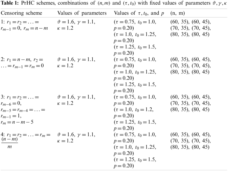
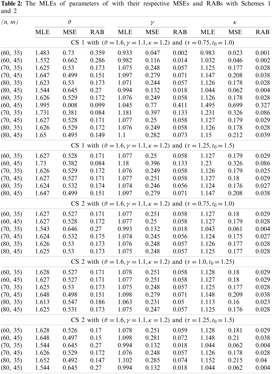
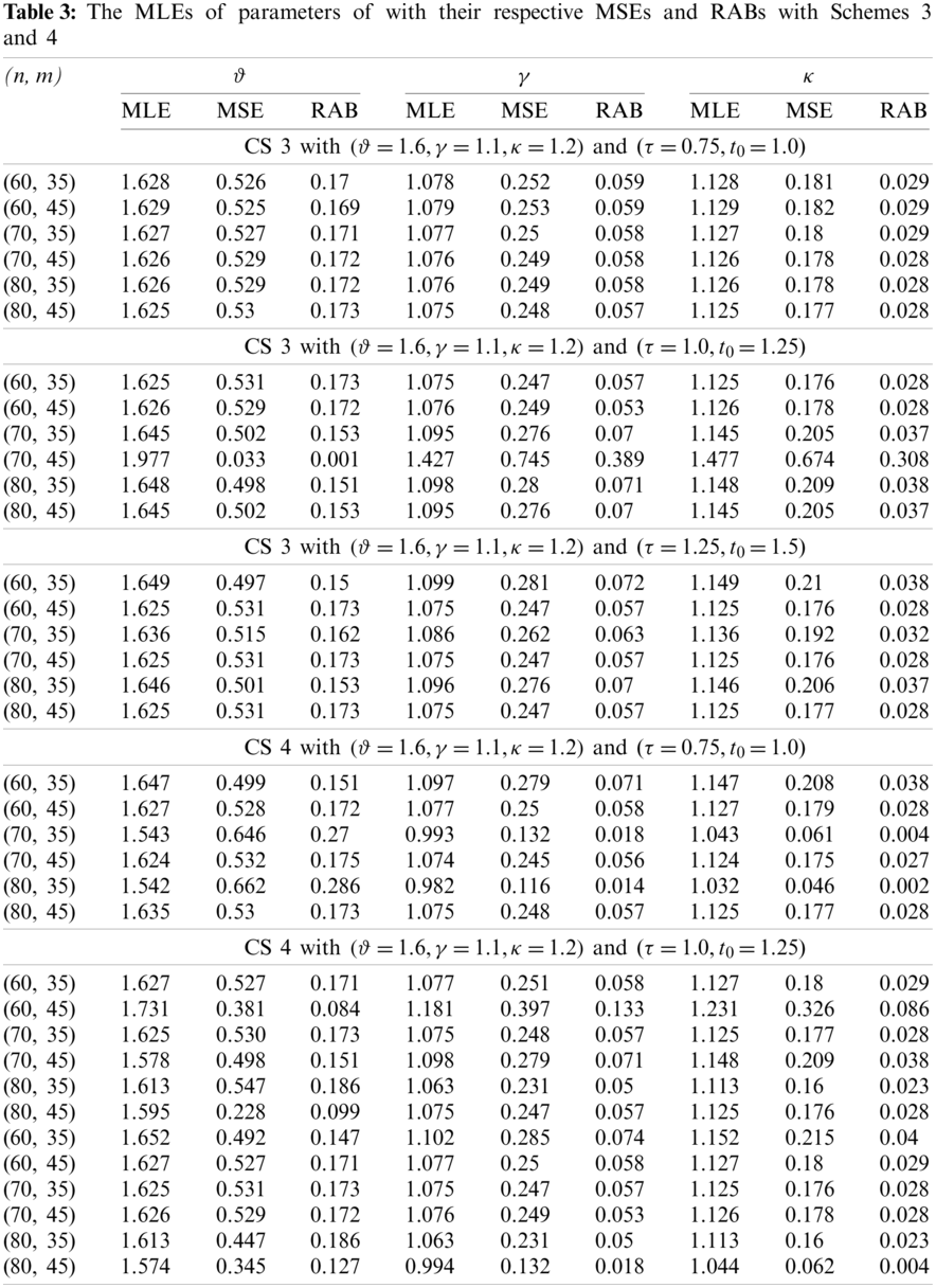
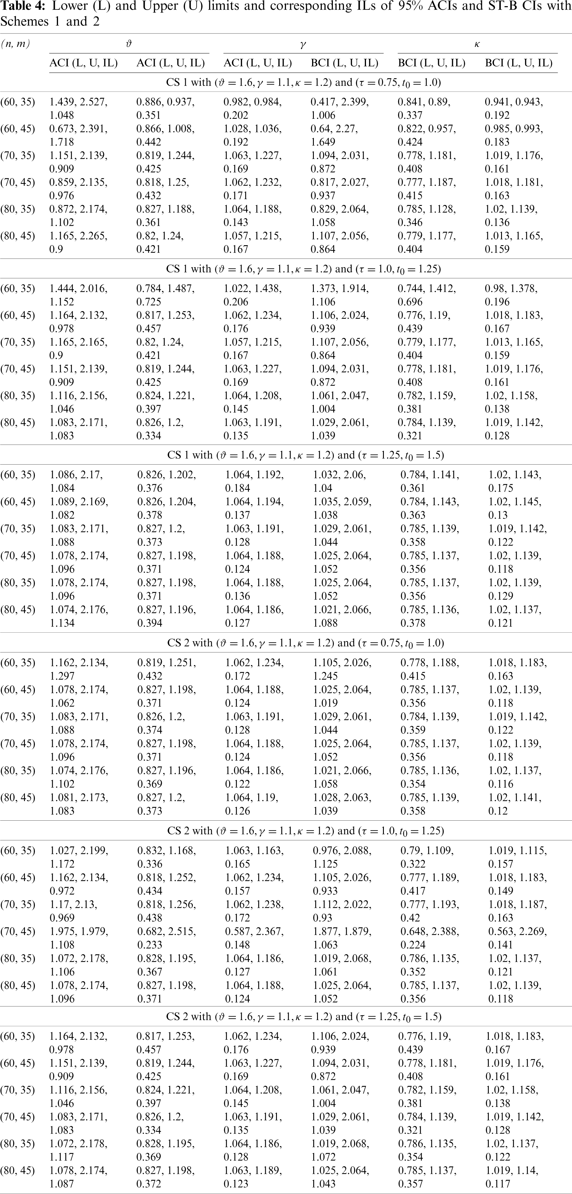
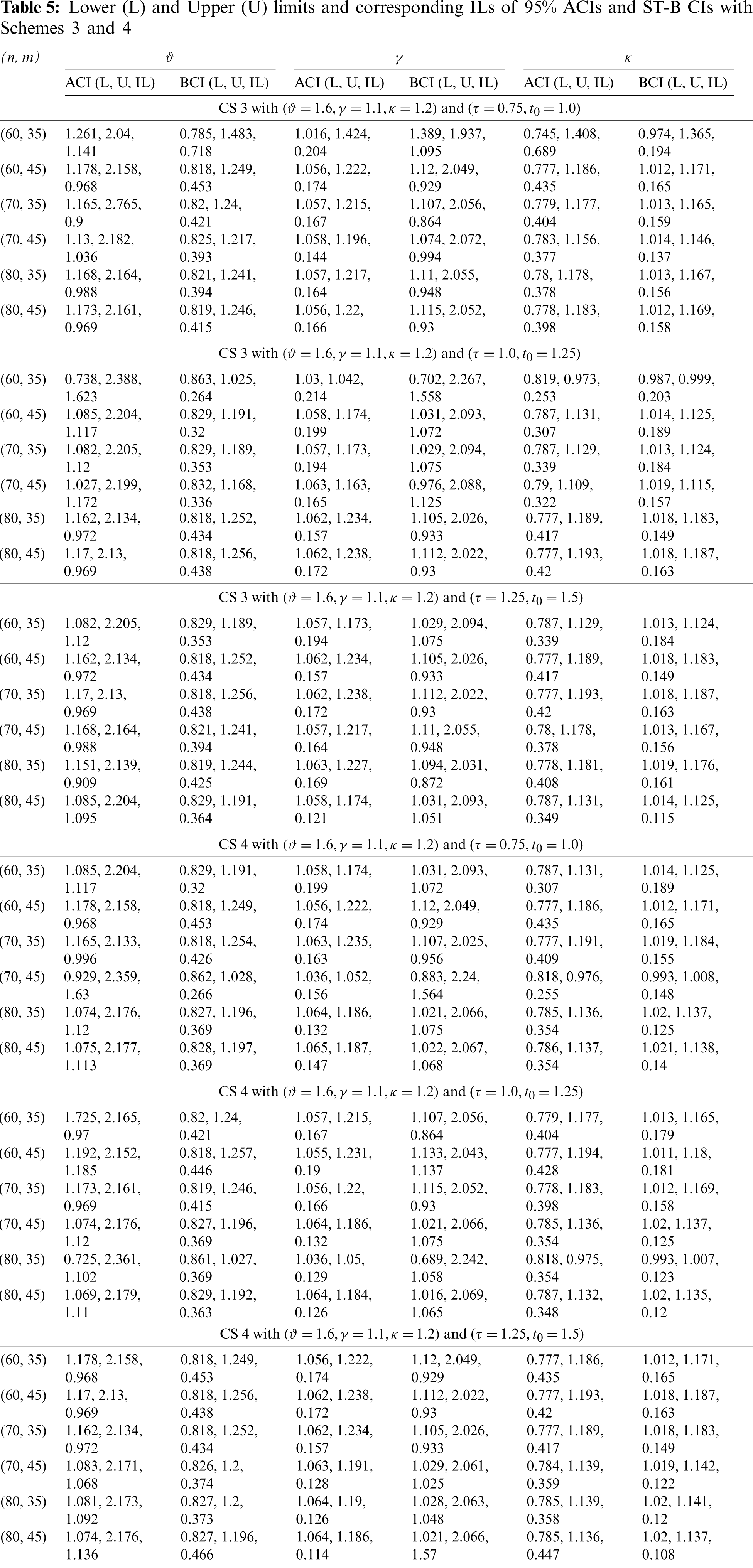
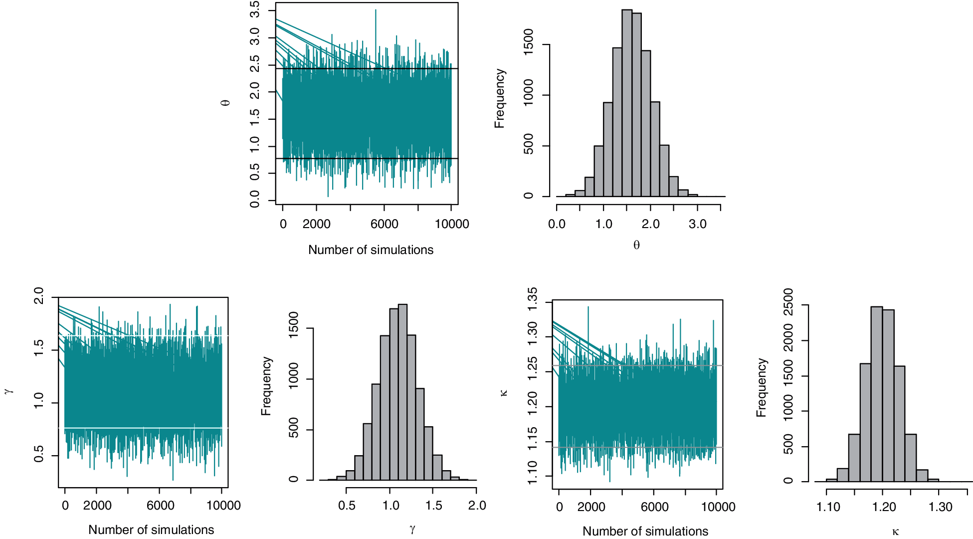
Figure 4: The plot of simulated samples and histogram of the parameters
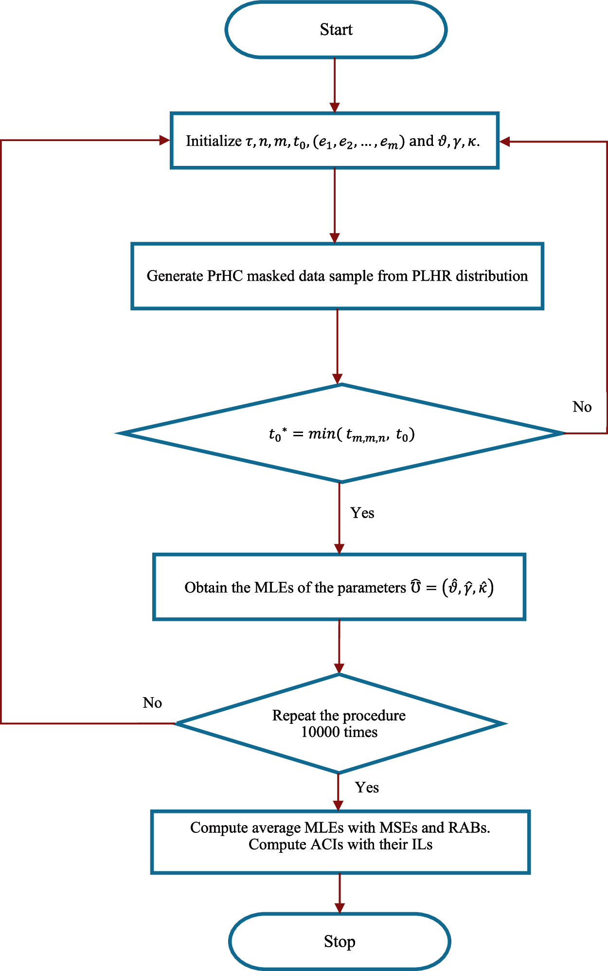
Figure 5: The flow chart to demonstrate the proposed estimation method
From the results listed in Tables 2 and 3, it can be observed that, for fixed
In this section, an actual data set is utilized to further illustrate the performance of the suggested estimation technique and to demonstrate the application of the PLHR distribution in practice in the field of reliability engineering. The R statistical programming language is used for computation. The dataset reported in Table 6 is an uncensored dataset consisting of real failure times of an airplane’s air conditioning systems (in hours) was first discussed by [68].
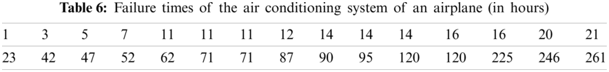
The Kolmogorov-Smirnov (K-S) goodness of fit test is used to fit the PLHR distribution to real data. The K-S test is used to compare a given data sample with a reference continuous probability distribution. It is based on the K-S distance, which is the absolute maximum distance between the sample’s empirical distribution function and the reference distribution’s cumulative distribution function and its corresponding p-value. In this current example, the K-S distance was determined to be 0.14146 with a p-value of 0.5856, which is greater than 0.05. Fig. 6 displays the plots of the empirical CDF vs. fitted CDF of PLHR distribution and histogram of data vs. fitted PDF of PLHR distribution. Consequently, it is evident from the K-S distance, p-value and Fig. 6 that the PHLR distribution and considered sample data tabulated in Table 6 both have the same probability distribution. Therefore, given data can be used as an illustration for our model.
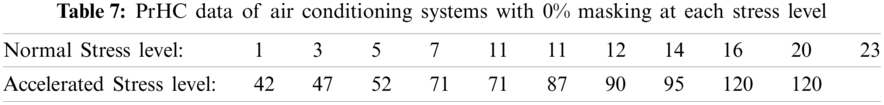
Now under SSPALT, for illustrative purposes, let’s consider the stress change time
For PrHC data in Table 7 with 0% masking under SSPALT, the MLEs of the parameters with initial values
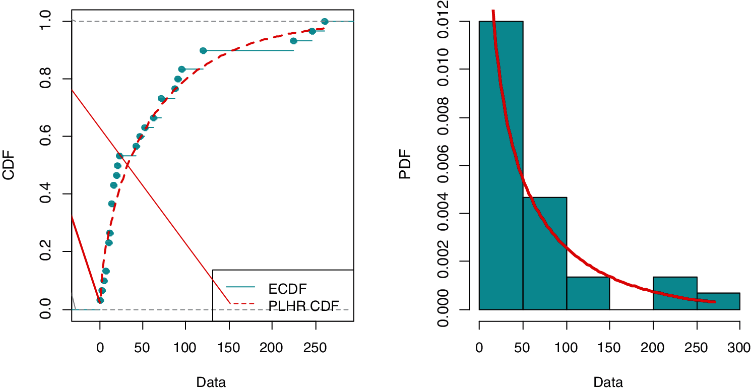
Figure 6: Plot of empirical CDF vs. PLHR CDF and histogram of data vs. fitted PDF of the PLHR distribution
Now, to demonstrate the effect of masking, at each stress level, 20% of failed systems are chosen at random to be masked. So, utilizing the data provided in Table 7 with 20% masking, the data obtained after masking with the PrHC scheme under SSPALT at each stress level is reported in the Table 8 as follows:
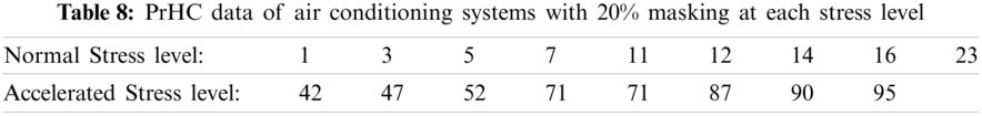
For PrHC data in Table 8 with 20% masking under SSPALT, we choose the same initial values of
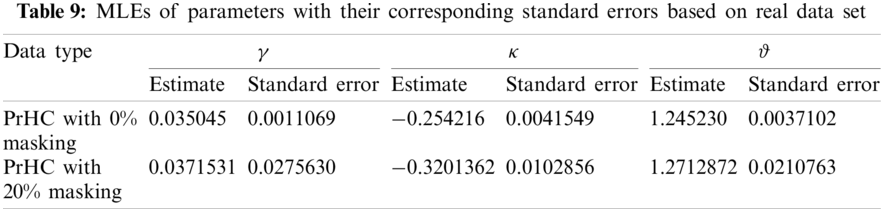
From Table 9, it can be observed that the ML estimates are more accurate with smaller standard errors when the sample size is large or the masking proportion is 0%, than the estimates under a smaller sample size or the masking level is 20%.
In this article, the SSPALT model has been developed for PrHC data to analyse the lifetime of a hybrid system of tree components under mask causes of failure. Assuming that the failure of components independently follows PLHR distribution, estimates of the parameters of PLHR distribution and the acceleration factor are then obtained using the MLE technique. The performance of MLEs is investigated through their respective MSEs and RABs. 95% ACIs and ST-B CIs are also constructed and their performance is investigated in terms of their respective ILs. A simulation study has also been conducted to investigate and compare the performance of estimates for the hybrid system under SSPALT for PrHC masked data by utilizing the Monte Carlo simulation technique. Additionally, a real-world data application for an airplane’s air conditioning systems was utilized to demonstrate the proposed approach. As a comparison between 95% ACIs and ST-B CIs, it is observed that the ST-B CIs provide narrower expected ILs in almost every case. Based on the findings, it can be concluded that the proposed model and method of estimation performed well. Hence all the statistical assumptions for fitting the model and regarding the estimation are satisfactory. As a future research project, the present study may be extended to more complex systems using the Bayesian estimation technique with different censored data.
Data Availability: The data used in this paper is available in the paper.
Funding Statement: The authors received no specific funding for this study.
Conflicts of Interest: The authors declare that they have no conflicts of interest to report regarding the present study.
1. Miyakawa, M. (1984). Analysis of incomplete data in competing risks model. IEEE Transactions on Reliability, 33(4), 293–296. DOI 10.1109/TR.1984.5221828. [Google Scholar] [CrossRef]
2. Usher, J. S., Hodgson, T. J. (1988). Maximum likelihood analysis of component reliability using masked system life-test data. IEEE Transactions on Reliability, 37(5), 550–555. DOI 10.1109/24.9880. [Google Scholar] [CrossRef]
3. Nelson, W. (1990). Accelerated testing: Statistical models, test plans and data analysis. New York: John Wiley & Sons. [Google Scholar]
4. Ma, H., Meeker, W. Q. (2010). Strategy for planning accelerated life tests with small sample sizes. IEEE Transactions on Reliability, 59(4), 610–619. DOI 10.1109/TR.2010.2083251. [Google Scholar] [CrossRef]
5. Li, X., Chen, W., Sun, F., Liao, H., Kang, R. et al. (2018). Bayesian accelerated acceptance sampling plans for a lognormal lifetime distribution under Type-I censoring. Reliability Engineering & System Safety, 171(3), 78–86. DOI 10.1016/j.ress.2017.11.012. [Google Scholar] [CrossRef]
6. Han, D., Bai, T. (2019). On the maximum likelihood estimation for progressively censored lifetimes from constant-stress and step-stress accelerated tests. Electronic Journal of Applied Statistical Analysis, 12(2), 392–404. DOI 10.1285/i20705948v12n2p392. [Google Scholar] [CrossRef]
7. Bai, X., Shi, Y., Ng, H. K. T. (2020). Statistical inference of Type-I progressively censored step-stress accelerated life test with dependent competing risks. Communications in Statistics-Theory and Methods, 1–27. DOI 10.1080/03610926.2020.1788081. [Google Scholar] [CrossRef]
8. Kamal, M., Rahman, A., Ansari, S. I., Zarrin, S. (2020). Statistical analysis and optimum step stress accelerated life test design for Nadarajah Haghighi distribution. Reliability: Theory & Applications, 15(4), 1–9. DOI 10.24411/1932-2321-2020-14005. [Google Scholar] [CrossRef]
9. Rahman, A., Sindhu, T. N., Lone, S. A., Kamal, M. (2020). Statistical inference for Burr Type X distribution using geometric process in accelerated life testing design for time censored data. Pakistan Journal of Statistics and Operation Research, 16(3), 577–586. DOI 10.18187/pjsor.v16i3.2252. [Google Scholar] [CrossRef]
10. Ma, Z., Liao, H., Ji, H., Wang, S., Yin, F. et al. (2021). Optimal design of hybrid accelerated test based on the inverse Gaussian process model. Reliability Engineering & System Safety, 210(2), 107509. DOI 10.1016/j.ress.2021.107509. [Google Scholar] [CrossRef]
11. Goel, P. K. (1971). Some estimation problems in the study of tampered random variables (Ph.D. Thesis). Department of Statistics, Carnegie Mellon University, Pittsburgh, Pennsylvania. [Google Scholar]
12. DeGroot, M. H., Goel, P. K. (1979). Bayesian estimation and optimal designs in partially accelerated life testing. Naval Research Logistics Quarterly, 26(2), 223–235. DOI 10.1002/(ISSN)1931-9193. [Google Scholar] [CrossRef]
13. Bhattacharyya, G. K., Soejoeti, Z. (1989). A tampered failure rate model for step-stress accelerated life test. Communications in Statistics-Theory and Methods, 18(5), 1627–1643. DOI 10.1080/03610928908829990. [Google Scholar] [CrossRef]
14. Bai, D. S., Chung, S. W. (1992). Optimal design of partially accelerated life tests for the exponential distribution under Type-I censoring. IEEE Transactions on Reliability, 41(3), 400–406. DOI 10.1109/24.159807. [Google Scholar] [CrossRef]
15. Bai, D. S., Chung, S. W., Chun, Y. R. (1993). Optimal design of partially accelerated life tests for the lognormal distribution under Type I censoring. Reliability Engineering & System Safety, 40(1), 85–92. DOI 10.1016/0951-8320(93)90122-F. [Google Scholar] [CrossRef]
16. Ismail, A. A. (2012). Inference in the generalized exponential distribution under partially accelerated tests with progressive Type-II censoring. Theoretical and Applied Fracture Mechanics, 59(1), 49–56. DOI 10.1016/j.tafmec.2012.05.007. [Google Scholar] [CrossRef]
17. Zhang, C., Shi, Y. (2016). Estimation of the extended Weibull parameters and acceleration factors in the step-stress accelerated life tests under an adaptive progressively hybrid censoring data. Journal of Statistical Computation and Simulation, 86(16), 3303–3314. DOI 10.1080/00949655.2016.1166366. [Google Scholar] [CrossRef]
18. Ismail, A. A. (2014). Inference for a step-stress partially accelerated life test model with an adaptive Type-II progressively hybrid censored data from Weibull distribution. Journal of Computational and Applied Mathematics, 260(2), 533–542. DOI 10.1016/j.cam.2013.10.014. [Google Scholar] [CrossRef]
19. Nassar, M., Nassr, S. G., Dey, S. (2017). Analysis of burr Type-XII distribution under step stress partially accelerated life tests with Type-I and adaptive Type-II progressively hybrid censoring schemes. Annals of Data Science, 4(2), 227–248. DOI 10.1007/s40745-017-0101-8. [Google Scholar] [CrossRef]
20. Mahmoud, M. A., Soliman, A. A., Abd Ellah, A. H., El-Sagheer, R. M. (2013). Estimation of generalized Pareto under an adaptive Type-II progressive censoring. Intelligent Information Management, 5(3), 73–83. DOI 10.4236/iim.2013.53008. [Google Scholar] [CrossRef]
21. Sobhi, M. M. A., Soliman, A. A. (2016). Estimation for the exponentiated Weibull model with adaptive Type-II progressive censored schemes. Applied Mathematical Modelling, 40(2), 1180–1192. DOI 10.1016/j.apm.2015.06.022. [Google Scholar] [CrossRef]
22. Hafez, E. H., Riad, F. H., Mubarak, S. A., Mohamed, M. S. (2020). Study on Lindley distribution accelerated life tests: Application and numerical simulation. Symmetry, 12(12), 2080. DOI 10.3390/sym12122080. [Google Scholar] [CrossRef]
23. Guess, F. M., Usher, J. S., Hodgson, T. J. (1991). Estimating system and component reliabilities under partial information on cause of failure. Journal of Statistical Planning & Inference, 29(1–2), 75–85. DOI 10.1016/0378-3758(92)90123-A. [Google Scholar] [CrossRef]
24. Doganaksoy, N. (1991). Interval estimation from censored and masked system-failure data. IEEE Transactions on Reliability, 40(3), 280–286. DOI 10.1109/24.85440. [Google Scholar] [CrossRef]
25. Lin, D. K., Usher, J. S., Guess, F. M. (1993). Exact maximum likelihood estimation using masked system data. IEEE Transactions on Reliability, 42(4), 631–635. DOI 10.1109/24.273596. [Google Scholar] [CrossRef]
26. Sarhan, A. M. (2001). Reliability estimation of components from masked system life data. Reliability Engineering & System Safety, 74(1), 107–113. DOI 10.1016/S0951-8320(01)00072-2. [Google Scholar] [CrossRef]
27. Flehinger, B. J., Reiser, B., Yashchin, E. (2002). Parametric modeling for survival with competing risks and masked failure causes. Lifetime Data Analysis, 8(2), 177–203. DOI 10.1023/A:1014891707936. [Google Scholar] [CrossRef]
28. Sarhan, A. M. (2003). Estimations of parameters in Pareto reliability model in the presence of masked data. Reliability Engineering & System Safety, 82(1), 75–83. DOI 10.1016/S0951-8320(03)00125-X. [Google Scholar] [CrossRef]
29. Sarhan, A. M. (2004). Parameter estimations in linear failure rate model using masked data. Applied Mathematics and Computation, 151(1), 233–249. DOI 10.1016/S0096-3003(03)00335-7. [Google Scholar] [CrossRef]
30. Tan, Z. (2005). Estimation of component failure probability from masked binomial system testing data. Reliability Engineering & System Safety, 88(3), 301–309. DOI 10.1016/j.ress.2004.08.013. [Google Scholar] [CrossRef]
31. Craiu, R. V., Reiser, B. (2006). Inference for the dependent competing risks model with masked causes of failure. Lifetime Data Analysis, 12(1), 21–33. DOI 10.1007/s10985-005-7218-3. [Google Scholar] [CrossRef]
32. Tan, Z. (2007). Estimation of exponential component reliability from uncertain life data in series and parallel systems. Reliability Engineering & System Safety, 92(2), 223–230. DOI 10.1016/j.ress.2005.12.010. [Google Scholar] [CrossRef]
33. Liu, Y., Shi, Y. (2010). Statistical analysis of the reliability for power supply of spacecraft with masked system life test data. Aerospace Control, 28(2), 70–74. [Google Scholar]
34. Reiser, B., Guttman, I., Lin, D. K., Guess, F. M., Usher, J. S. (1995). Bayesian inference for masked system lifetime data. Journal of the Royal Statistical Society: Series C (Applied Statistics), 44(1), 79–90. DOI 10.2307/2986196. [Google Scholar] [CrossRef]
35. Lin, D. K. J., Usher, J. S., Guess, F. M. (1996). Bayes estimation of component-reliability from masked system-life data. IEEE Transactions on Reliability, 45(2), 233–237. DOI 10.1109/24.510807. [Google Scholar] [CrossRef]
36. Kuo, L., Yang, T. Y. (2000). Bayesian reliability modeling for masked system lifetime data. Statistics & Probability Letters, 47(3), 229–241. DOI 10.1016/S0167-7152(99)00160-1. [Google Scholar] [CrossRef]
37. Sarhan, A. M. (2001). The Bayes procedure in exponential reliability family models using conjugate convex tent prior family. Reliability Engineering & System Safety, 71(1), 97–102. DOI 10.1016/S0951-8320(00)00086-7. [Google Scholar] [CrossRef]
38. Basu, S., Sen, A., Banerjee, M. (2003). Bayesian analysis of competing risks with partially masked cause of failure. Journal of the Royal Statistical Society: Series C (Applied Statistics), 52(1), 77–93. DOI 10.1111/1467-9876.00390. [Google Scholar] [CrossRef]
39. Mukhopadhyay, C., Basu, S. (2007). Bayesian analysis of masked series system lifetime data. Communications in Statistics–-Theory and Methods, 36(2), 329–348. DOI 10.1080/03610920600853357. [Google Scholar] [CrossRef]
40. Xu, A., Tang, Y. (2011). Nonparametric Bayesian analysis of competing risks problem with masked data. Communications in Statistics–Theory and Methods, 40(13), 2326–2336. DOI 10.1080/03610921003786830. [Google Scholar] [CrossRef]
41. Sarhan, A. M., Kundu, D. (2008). Bayes estimators for reliability measures in geometric distribution model using masked system life test data. Computational Statistics & Data Analysis, 52(4), 1821–1836. DOI 10.1016/j.csda.2007.05.031. [Google Scholar] [CrossRef]
42. Yousif, Y., Elfaki, F. A., Hrairi, M., Adegboye, O. A. (2020). A Bayesian approach to competing risks model with masked causes of failure and incomplete failure times. Mathematical Problems in Engineering, 2020, 1–7. DOI 10.1155/2020/8248640. [Google Scholar] [CrossRef]
43. Cai, J., Shi, Y., Liu, B. (2017). Statistical analysis for masked system life data from Marshall-Olkin Weibull distribution under progressive hybrid censoring. Naval Research Logistics, 64(6), 490–501. DOI 10.1002/nav.21769. [Google Scholar] [CrossRef]
44. Peng, W., Huang, H. Z., Xie, M., Yang, Y., Liu, Y. (2013). A Bayesian approach for system reliability analysis with multilevel pass-fail, lifetime and degradation data sets. IEEE Transactions on Reliability, 62(3), 689–699. DOI 10.1109/TR.2013.2270424. [Google Scholar] [CrossRef]
45. Yang, L., Guo, Y., Wang, Q. (2020). Reliability assessment of a hierarchical system subjected to inconsistent priors and multilevel data. IEEE Transactions on Reliability, 69(1), 277–292. DOI 10.1109/TR.2019.2895501. [Google Scholar] [CrossRef]
46. Yang, L., Wang, P., Wang, Q., Bi, S., Peng, R. et al. (2021). Reliability analysis of a complex system with hybrid structures and multi-level dependent life metrics. Reliability Engineering & System Safety, 209(1–2), 107469. DOI 10.1016/j.ress.2021.107469. [Google Scholar] [CrossRef]
47. Wang, R., Sha, N., Gu, B., Xu, X. (2015). Parameter inference in a hybrid system with masked data. IEEE Transactions on Reliability, 64(2), 636–644. DOI 10.1109/TR.2015.2412537. [Google Scholar] [CrossRef]
48. Sha, N., Wang, R., Hu, P., Xu, X. (2015). Statistical inference in dependent component hybrid systems with masked data. Advances in Statistics, 2015, 525136. DOI 10.1155/2015/525136. [Google Scholar] [CrossRef]
49. Cai, J., Shi, Y., Bai, X. (2017). Statistical analysis of masked data in a hybrid system based on copula theory under progressive hybrid censoring. Sequential Analysis, 36(2), 240–250. DOI 10.1080/07474946.2017.1319686. [Google Scholar] [CrossRef]
50. Rodrigues, A. S., Pereira, C. A. D. B., Polpo, A. (2019). Estimation of component reliability in coherent systems with masked data. IEEE Access, 7, 57476–57487. DOI 10.1109/ACCESS.2019.2913675. [Google Scholar] [CrossRef]
51. Shi, X., Zhan, P., Shi, Y. (2020). Statistical inference for a hybrid system model with incomplete observed data under adaptive progressive hybrid censoring. Concurrency and Computation: Practice and Experience, 32(14), e5708. DOI 10.1002/cpe.5708. [Google Scholar] [CrossRef]
52. Fan, T. H., Wang, W. L. (2011). Accelerated life tests for Weibull series systems with masked data. IEEE Transactions on Reliability, 60(3), 557–569. DOI 10.1109/TR.2011.2134270. [Google Scholar] [CrossRef]
53. Fan, T. H., Hsu, T. M. (2012). Accelerated life tests of a series system with masked interval data under exponential lifetime distributions. IEEE Transactions on Reliability, 61(3), 798–808. DOI 10.1109/TR.2012.2209259. [Google Scholar] [CrossRef]
54. Xu, A., Basu, S., Tang, Y. (2014). A full Bayesian approach for masked data in step-stress accelerated life testing. IEEE Transactions on Reliability, 63(3), 798–806. DOI 10.1109/TR.2014.2315940. [Google Scholar] [CrossRef]
55. Xu, A., Tang, Y., Guan, Q. (2014). Bayesian analysis of masked data in step-stress accelerated life testing. Communications in Statistics-Simulation and Computation, 43(8), 2016–2030. DOI 10.1080/03610918.2013.848894. [Google Scholar] [CrossRef]
56. Shi, X., Liu, Y., Shi, Y. (2017). Statistical analysis for masked hybrid system lifetime data in step-stress partially accelerated life test with progressive hybrid censoring. PLOS One, 12(10), e0186417. DOI 10.1371/journal.pone.0186417. [Google Scholar] [CrossRef]
57. Shi, X., Shi, Y., Song, Q. (2018). Inference for four-unit hybrid system with masked data under partially acceleration life test. Systems Science & Control Engineering, 6(1), 195–206. DOI 10.1080/21642583.2018.1474503. [Google Scholar] [CrossRef]
58. Shi, X. L., Lu, P., Shi, Y. M. (2018). Inference and optimal design on step-stress partially accelerated life test for hybrid system with masked data. Journal of Systems Engineering and Electronics, 29(5), 1089–1100. DOI 10.21629/JSEE.2018.05.19. [Google Scholar] [CrossRef]
59. Rinne, H. (2014). The hazard rate: Theory and inference (with supplementary MATLAB-programs). Justus-Liebig-University, Germany. http://geb.uni-giessen.de/geb/volltexte/2014/10793/. [Google Scholar]
60. Tarvirdizade, B., Nematollahi, N. (2019). The power-linear hazard rate distribution and estimation of its parameters under progressively Type-II censoring. Hacettepe Journal of Mathematics and Statistics, 48(3), 818–844. DOI 10.15672/HJMS.2018.608. [Google Scholar] [CrossRef]
61. Kundu, D., Joarder, A. (2006). Analysis of Type-II progressively hybrid censored data. Computational Statistics & Data Analysis, 50(10), 2509–2528. DOI 10.1016/j.csda.2005.05.002. [Google Scholar] [CrossRef]
62. Balakrishnan, N. (2007). Progressive censoring methodology: An appraisal. Test, 16(2), 211–296. DOI 10.1007/s11749-007-0061-y. [Google Scholar] [CrossRef]
63. Balakrishnan, N., Kundu, D. (2013). Hybrid censoring: Models, inferential results and applications. Computational Statistics & Data Analysis, 57(1), 166–209. DOI 10.1016/j.csda.2012.03.025. [Google Scholar] [CrossRef]
64. Efron, B. (1982). The jackknife, the bootstrap and other resampling plans. Philadelphia, PA, USA: Society for Industrial and Applied Mathematics. [Google Scholar]
65. Hall, P. (1988). Theoretical comparison of bootstrap confidence intervals. The Annals of Statistics, 16(3), 927–953. DOI 10.1214/aos/1176350933. [Google Scholar] [CrossRef]
66. Efron, B., Tibshirani, R. J. (1993). An introduction to the bootstrap (1st ed.). London, UK: Chapman and Hall/CRC. DOI 10.1201/9780429246593. [Google Scholar] [CrossRef]
67. Balakrishnan, N., Sandhu, R. A. (1995). A simple simulation algorithm for generating progressive Type-II censored samples. The American Statistician, 49(2), 229–230. DOI 10.1080/00031305.1995.10476150. [Google Scholar] [CrossRef]
68. Linhart, H., Zucchini, W. (1986). Model selection. New York: Wiley. [Google Scholar]
Elements of F are:
where,
 | This work is licensed under a Creative Commons Attribution 4.0 International License, which permits unrestricted use, distribution, and reproduction in any medium, provided the original work is properly cited. |