Computer Modeling in Engineering & Sciences

DOI: 10.32604/cmes.2022.018480

ARTICLE

A Fast Approach for Predicting Aerodynamic Noise Sources of High-Speed Train Running in Tunnel

Deng Qin1, Tian Li1,*, Honglin Wang2, Jizhong Yang3, Yao Jiang3, Jiye Zhang1 and Haiquan Bi2

1State Key Laboratory of Traction Power, Southwest Jiaotong University, Chengdu, 610031, China
2School of Mechanical Engineering, Southwest Jiaotong University, Chengdu, 610031, China
3China Railway Eryuan Engineering Group Co., Ltd., Chengdu, 610031, China
*Corresponding Author: Tian Li. Email: litian2008@swjtu.edu.cn
Received: 28 July 2021; Accepted: 14 October 2021

1  Introduction

With the continuous development of high-speed railways, there are many operating environments for high-speed trains. Tunnels are one of the major routes of high-speed trains. When high-speed trains pass through tunnels, complex aerodynamic effects, along with noise problems will occur [1–3]. The sound generated by the high-speed train passing through a tunnel will create a large noise action by the multiple waves’ reflections and superposition. The noise in tunnels is much larger than that in the open air. Therefore, an in depth study of the aerodynamic noise characteristics of high-speed trains passing through tunnels is of great importance for the reduction of aerodynamic noises.

Current research mainly focuses on the identification of aerodynamic noise sources, including noise mechanisms and characteristics, and noise optimization when high-speed trains are running on open tracks [4]. Therefore, the aerodynamic noise characteristics and sounding mechanism of high-speed trains running on open tracks have been described. When the train's speed exceeds 300 km/h, aerodynamic noise will become the dominant noise. Meanwhile, high-speed train aerodynamic noise is still dominated by dipole noise [5–7]. The main sources of aerodynamic noise for high-speed trains are the streamlined nose of the head and tail cars, bogies, pantograph, air conditioners, and windshields [8–11]. These complex structures form more prominent sound sources, such as cavity noise, vortex shedding, flow separation and vehicle body boundary layer noise. They are composed of sound source distributions of different phases and amplitudes, mostly broadband noise and turbulence noise. This adds complexity to its noise prediction. Usually, people understand the source of aerodynamic noise by studying the flow around a high-speed train and the pressure pulsation in the near field.

The head and tail cars of high-speed trains have the same streamlined nose. However, their sound mechanisms are different [12,13]. When high-speed air flows over the streamlined nose of the head car, it firstly stagnates at the tip of the nose, after which, the flow accelerates. The airflow is significantly disturbed, the airflow in the boundary layer near the train is highly turbulent, and the fluctuating pressure on the surface of the head car is greater, forming a high-noise area in the local area. In addition, the flow separation and reattachment tend to occur near the plough and the cab windows. When high-speed air flows over the streamlined nose, the boundary layer above the nose becomes thicker, and the flow separation and reattachment phenomena around the streamlined nose are complicated. The airflow separation from the tail car and shedding vortex with opposite rotations are the main mechanisms for generating aerodynamic noise in the wake of the train. As the bogie and its surrounding cabin are complex, the high-speed air flows over the bogie cabin. The complex flow in the cabin forms a very strong aerodynamic noise [14–16]. In addition, the pantograph is composed of multiple rods. The airflow separation, vortex shedding and interaction around the rods are the main causes of aerodynamic noise induced by the pantograph. The vortex shedding generates periodic forces on the rods, forming a strong dipole sound source, and making aerodynamic noise, with the vortex shedding frequency as the peak frequency [17–20]. Besides, an annular cavity exists around the windshield. When airflow goes over the cavity, a large velocity gradient exists at the front of the cavity. A strong three-dimensional vortex around the inner windshield in the cavity is formed. Small vortices with different sizes will cause a strong noise around the windshield [21,22].

Up to now, many scholars have studied the aerodynamic noise of high-speed trains passing through tunnels. However, most of the research focuses on the internal noise of the train, while relatively few studies address external noise and aerodynamic noise sources. Li et al. [23] systematically studied aerodynamic characteristics of a high-speed train in three situations, comprising open air, entering a tunnel and completely in a tunnel. The results show that the internal noise of the high-speed train in the tunnel is the largest. Zhang et al. [24] studied the interior noise characteristics of high-speed trains under several typical operating conditions, including slab track, ballast track, open air, and tunnel. The results show that the track form has a small impact on the internal noise of high-speed trains, while the tunnel has a greater impact on the internal noise. Tan et al. [25] used a numerical wind tunnel model and non-reflective boundary conditions to study the aerodynamic noise sources of high-speed trains in tunnels. The results show that the spectrum pattern of the sound source energy presented broadband characteristics for the high-speed train. The dominant distribution frequency range is from 100 Hz to 4 kHz for the high-speed train, accounting for approximately 95.1% of the total sound source energy. It can be seen that the aerodynamic noise problem of high-speed trains passing through tunnels is more serious. The key issue is to analyze the characteristics of aerodynamic noise sources of high-speed trains in tunnels.

However, High-speed trains are affected by pressure waves when running in tunnels, and the flow around the train is more complex. It is difficult to numerically simulate the aerodynamic noise of high-speed trains running in tunnels. There are two typical methods. One is the numerical wind tunnel method based on the principle of relative motion combined with non-reflective boundary conditions. The non-reflective boundary conditions can effectively solve the problem of pseudo-reflected waves caused by the artificial truncation of the calculation domain, thereby eliminating the influence of the pressure wave in the tunnel on the characteristics of the surface noise source of the train. The other method is a dynamic mesh method, combined with an adaptive grid. This directly uses high-precision algorithms and high-quality grids to solve the fluctuating pressure characteristics of the train surface, when the high-speed train passes through the tunnel. In this paper, the above two different methods are used to study the flow structures and aerodynamic noise sources when the high-speed train is running in a tunnel.

2  Governing Equations

2.1 Improved Delayed Detached Eddy Simulation (IDDES)

Detached Eddy Simulation (DES) is a hybrid method that combines the advantages of Unsteady Reynolds Average Navier-Stokes (URANS) and Large Eddy Simulation (LES). URANS is used in the boundary layer, and the LES is used in the other regions. This reduces the required computing resources, while ensuring a high calculation accuracy. At present, improved delayed detached eddy simulation (IDDES) based on the SST k-ω turbulence model is widely used to simulate the turbulent flow around high-speed trains [26–28]. The transport equations for SST k-ω model are given in detail in [29]. The transport equations for IDDES are given in detail in [30]. The operating speed of the high-speed train in this study is 350 km/h. Although the operating speed is less than 0.3 Ma, the change in the air density when a high-speed train runs in the tunnel cannot be ignored.

2.2 Aeroacoustic Equation

Lighthill acoustic analogy theory divides the sound sources into three categories, comprising monopole noise sources, dipole noise sources and quadrupole noise sources [31,32]. The aerodynamic noise of a high-speed train is mainly the dipole noise, which is determined by the aerodynamic behavior of solid surfaces. The Curle acoustic integral formula can solve the dipole noise generated by the flow over the solid surface. The acoustic integral formula is as follows,

ps(x,t)=14πc0∫S[cos⁡(θ)r∂p∂t(y,τ)]dS(y)(1)

where ps is the sound pressure, x and y are the spatial position vectors of the noise evaluation point and the noise source respectively, c0 is the speed of sound, θ is the angle between the surface normal vector of the sound source and the vector from the sound source to the noise evaluation point, r is the distance from the sound source to the noise evaluation point, τ is the delay time, S is the surface area of the sound source, p is the pulsating pressure on the train surface.

The relationship between the acoustic energy density of far-field aerodynamic noise and sound pressure is as follows

I=ps2(x,t)¯ρ0c0=116π2ρ0c03(∫Scos⁡θr∂p∂t(y,τ)dS(y))2¯(2)

Treating the sound source as a point sound source, and neglecting the influence of the delay time at a low Mach number, the total sound power radiated by the sound source can be determined by

W=4πr2I=14πρ0c03(∂∂t∫Sp(y)dS(y))2¯(3)

We define

F=∫Sp(y)dS(y)(4)

Subsequently, we have

W∝F′2¯(5)

where the overline represents the average value of the physical quantity in the time domain, W is the sound source power, the right superscript ′ represents the time derivative and F is the pulsating pressure.

The sound power per unit area (unit: W/m2) described by the sound power level is expressed as

SAP=10logWWref(6)

where Wref represents the reference sound power, which is 1 × 10−12 W.

The sound pressure level is defined as

SPL=20logppref(7)

where pref represents the reference sound pressure, which is 2 × 10−5 Pa.

3  Numerical Details

3.1 Model Geometry

A typical high-speed train is chosen as the research object, with a simplified bogie cabin and pantograph. The streamlined nose and train body are unchanged. The simplified geometric model is shown in Fig. 1. The train consists of a head car and a tail car. The head and tail cars have the same streamlined nose. The total length of the train is L =50.8 m. The height H =3.5 m.

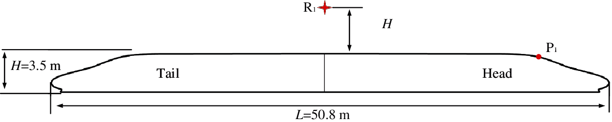
Figure 1: Numerical model

3.2 Computational Domain and Boundary Conditions

Fig. 2 shows the computational domain when the numerical static method (Method 1) is used. Similar to a wind tunnel, the train is stationary and the fluid is moving. The length of the tunnel is 20 L, the diameter of the tunnel is 2.5 H, and the bottom surface of the train is about 0.1 H height above the ground. The setting of the boundary conditions is similar to that of static experiments. The inlet is set as a pressure inlet and non-reflective boundary condition. The outlet is set as a pressure outlet and non-reflective boundary condition. The ground and ceiling of the tunnel are set as sliding wall boundaries, which are used to simulate an infinitely long tunnel. The sliding speed is 350 km/h. The train is set as a non-slip wall boundary.

Figure 2: Computational domain based on Method 1

Fig. 3 shows the computational domain when the dynamic mesh method (Method 2) is used. The train is moving at a speed of 350 km/h. The tunnel length is 20 L and the tunnel diameter is 2.5 H. The boundaries A, B, E, and F are all set as pressure outlets. The boundaries C, D and the ceiling of the tunnel are set as a non-slip wall boundary, which is used to simulate a real tunnel wall environment. The train is set as a non-slip moving wall with a speed of 350 km/h. The movement of the train is achieved using a custom UDF file.

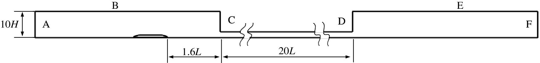
Figure 3: Computational domain based on Method 2

3.3 Computational Mesh

The computational domain based on Method 1 is selected to test the mesh independence, in which different basic size discretization calculation domains were set, and three sets of grids with different grid quantities of 18.24 million, 21.44 million and 27.65 million were obtained. Fig. 4 shows the comparison result of the wake speed of the train with different grid quantities. It can be seen from the figure that the time-averaged velocity amplitude distributions of the 40 measuring points of the train wake are basically the same. Compared with the fine grid, the calculation results of the medium grid have very little variation. Therefore, the medium grid is selected for subsequent calculations.

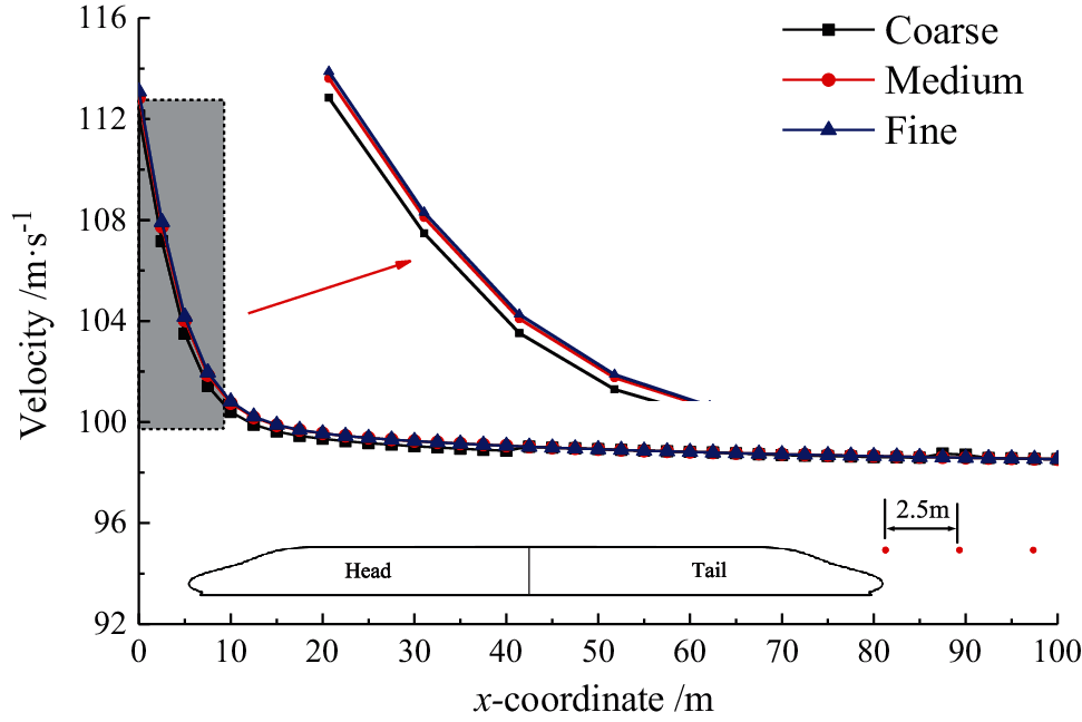
Figure 4: Mesh independence test

The computational domain is discretized using an unstructured hexahedral grid of the same size. The computational mesh is shown in Fig. 5. The mesh around the high-speed train is refined. In order to capture the flow details around the train, a detailed boundary layer is used, as shown in Fig. 5b. The height of the first cell above the wall is 0.04 mm, the expansion ratio is 1.2 and the total number of boundary layers is 16. Such boundary layers make the y+ on the train approximately equal to 1. The total number of grids is 21.44 million and 28.12 million for computational domains based on Method 1 and Method 2, respectively.

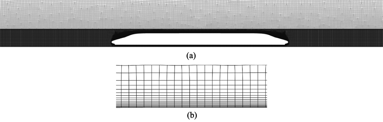
Figure 5: Computational grid (a) Grid around the train (b) Boundary layer grid

3.4 Numerical Method and Validation

When Method 1 is used to simulate the flow around trains, the procedure is as follows. First, the SST k-ω turbulence model is used to calculate the steady flow field. Then, the obtained steady flow field is taken as the initial flow field of the unsteady flow field calculation, and the transient flow field is solved using IDDES. Third, when the physical quantity of the flow field changes periodically, the time-averaged physical quantity of the flow field in a certain period of time is measured. For the dynamic mesh method, IDDES is used directly to solve the transient flow field.

In order to compare the two above methods, the implicit density solver is adopted. Meanwhile, the advection upstream splitting method+ (ASUM+) is adopted for the flux, and the flow and turbulence terms are all found using the second order upwind scheme (SOUS). In terms of time discretization, the implicit time step method is adopted. The physical time step adopts the second order Euler backward scheme (SOEBS), and the internal iteration adopts the implicit time-marching scheme (ITMS). The time steps are all set to 1 × 10−4 s. The maximum resolvable frequency is 5 kHz.

In order to verify the rationality and correctness of the numerical calculation method in this paper, a 1/8 scaled high-speed train aerodynamic noise wind tunnel test was carried out. During the wind tunnel test, 30 microphones were arranged on one side of the train model to measure the aerodynamic noise of the train. The distance between the microphone and the track centerline was 5.8 m. The test model was a smooth car body, and the bogie and pantograph areas were filled with blocking blocks, as shown in Fig. 6.

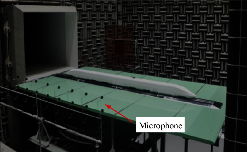
Figure 6: Wind tunnel test

The wind tunnel test can verify the correctness of the numerical static calculation method (Method 1). Therefore, the same numerical simulation calculation model as used in the wind tunnel test was set up. Fig. 7 shows the comparison result of the arithmetic mean of the sound pressure levels at the 30 microphones. The results of the numerical simulation and the wind tunnel test are in good agreement. Affected by the surface layer during the test, the test results under different wind speeds are larger than the simulation calculation results, the maximum difference being 1.37 dBA. In general, numerical simulation has high calculation accuracy.

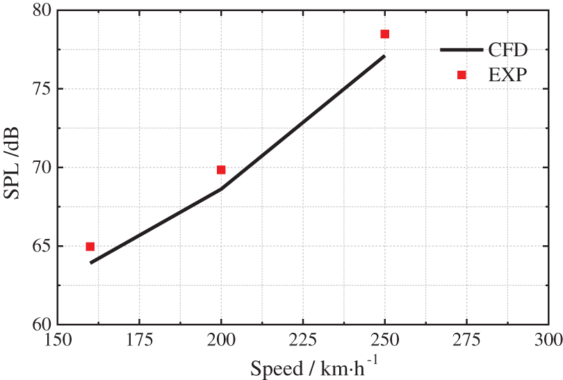
Figure 7: Comparison results of numerical simulation and experiment

4  Results

The results will be discussed and analyzed in terms of surface pressure, flow field and aerodynamic noise source.

4.1 Surface Pressure

Fig. 8 shows the time-varying pressure curves of the train surface measuring point P1 (the location is shown in Fig. 1), calculated by two different computational methods. It can be seen from Fig. 8a that the surface pressure of the train has a strong unsteady characteristic, and the pressure at the measuring point presents periodic fluctuations. It can be seen from Fig. 8b that high-speed trains will generate pressure waves when running in tunnels. The existence of pressure waves will seriously affect the pressure amplitude on the train surface, and there will still be strong unsteady characteristics on the train surface. Time t1 in the figure represents the moment the head car enters the tunnel. At that moment, a compression wave will be generated and the amplitude of the surface pressure of the train will increase. Time t2 represents when the tail car starts entering the tunnel. At this time, an expansion wave will be generated and the amplitude of the surface pressure of the train will decrease. The compression and expansion waves propagate back and forth in the tunnel at the speed of sound. When the train has completely entered the tunnel and the waves are not reflected at the exit, the time-averaged pressure amplitude on the train surface does not change significantly, seen in the pressure results during the time interval between 2.0  and 2.5 s.

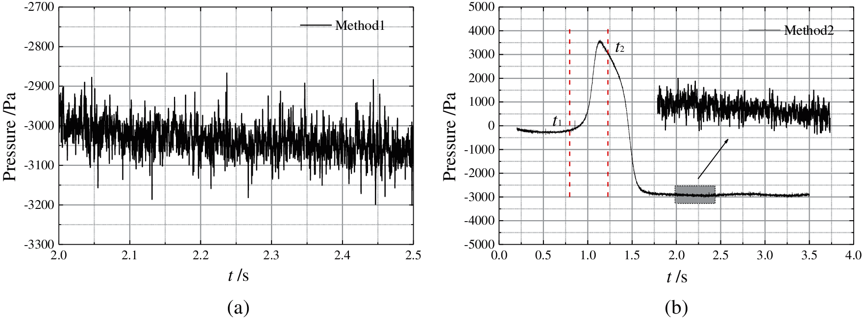
Figure 8: Time history curve of the fluctuating pressure (a) Method 1 (b) Method 2

The time-averaged pressure reflects the statistically stable value of the time-varying pressure over a period of time. In addition, the fast Fourier transform of the time-varying pressure data collected at the measurement point P1 within a certain period of time (2.0∼2.5 s) can obtain and analyze the frequency spectrum of the pulsating pressure. Fig. 9 shows the frequency spectrum characteristics of the pressure at P1 for the two methods during 0.5 s. It can be seen from the figure that the power spectral density (PSD) of the fluctuating pressure on the train surface is basically the same for both methods, but that there is a certain difference in the energy in the low frequency range. For Method 2, the pressure wave generated by the high-speed train entering the tunnel increases the energy of the surface pressure on the train in the lower frequency range.

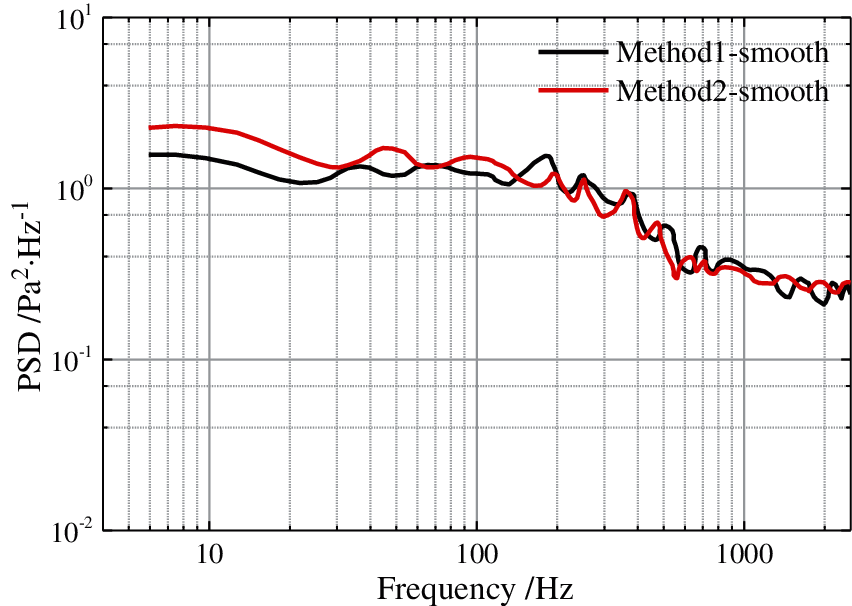
Figure 9: Power spectral density at measuring point P1

Fig. 10 shows the time-averaged pressure during the period from 2.0 to 2.5 s when the high-speed train is running in the tunnel for Method 1 and Method 2. It can be seen that the distribution characteristics of the pressure around the high-speed train for both methods are basically the same, and there are certain differences in some local regions, such as the regions around the tail nose. Comparing the pressure distribution around the head and tail cars, the pressure contours around the head car are basically the same when using different calculation methods. However, the pressure contours around the tail car show a certain difference. For Method 2, the wake flow around the tail car are captured in more detail, and the pressure contours are more hierarchical. Fig. 11 shows the comparison of the time-averaged pressure amplitude on the central cross-section of the high-speed train. It can be seen that the difference in the time-averaged pressure amplitudes of the head car surface obtained using the two calculation methods are relatively small, less than 5%. However, the time-averaged pressure amplitude on the tail car shows a greater difference, of nearly 10% in most regions.

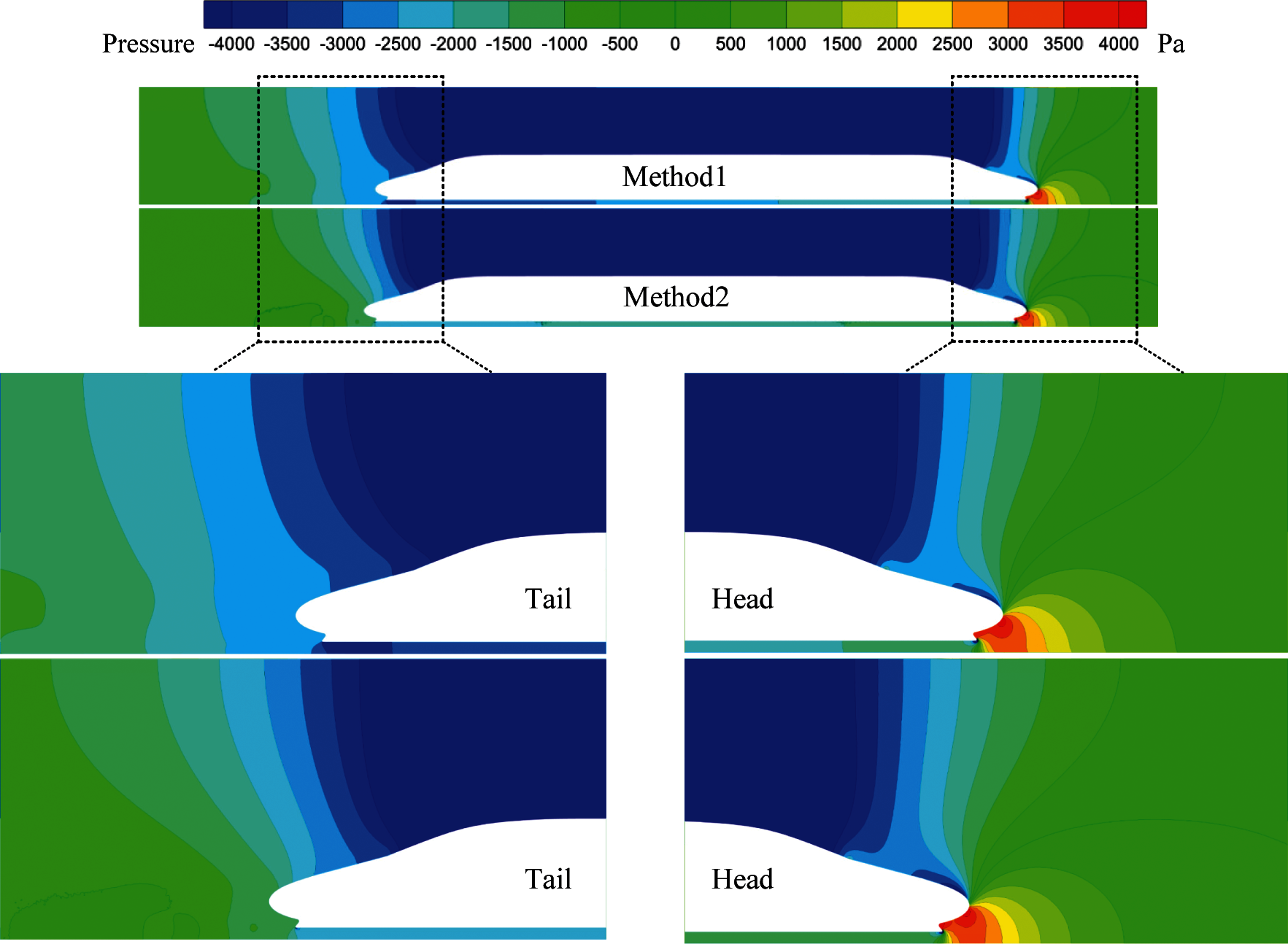
Figure 10: Time-averaged pressure around the train

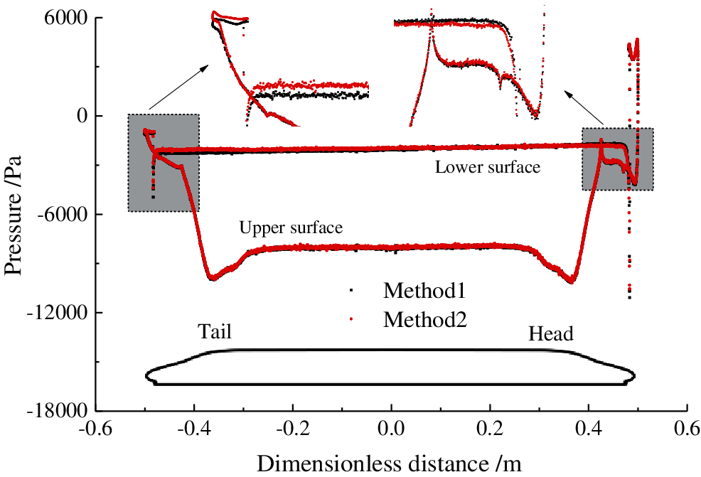
Figure 11: Time-averaged pressure on the train surface

4.2 Flow Field

Accurately predicting the fluctuating pressure on the train body is a key to the identification of the aerodynamic noise sources generated by the high-speed train. It can be evaluated by the physical quantities of the 0th, 1st and 2nd order of the flow field. The vorticity is a linear function of the first derivative of velocity, and the Q value is the squared difference of the second norm of the vorticity tensor and the strain rate tensor. Therefore, comparative analysis of flow field velocity, vorticity and Q value can show the differences in results obtained using different methods.

Fig. 12 shows the time-averaged velocity magnitude at the central cross-section. The results obtained using Method 1 are based on the principle of relative motion. In order to facilitate comparison with results found using Method 2, the vector result obtained using Method 1 is transformed. It can be seen that when the train is running, the surrounding flow will move. In the upstream region of the train nose tip, the airflow velocity is relatively high, due to existence of the train. In the wake of the train, the surrounding flow will quickly rush into and occupy the region. Therefore, the flow velocity is also relatively high. For the two calculation methods, the time-averaged velocity around high-speed trains running in the tunnel is basically the same. However, the time-averaged velocity in certain regions is different. For the static method, the time-averaged velocity around the head car nose is smaller, while that around the tail car is relatively larger. Moreover, the area with high velocity is also larger than that using the dynamic mesh method.

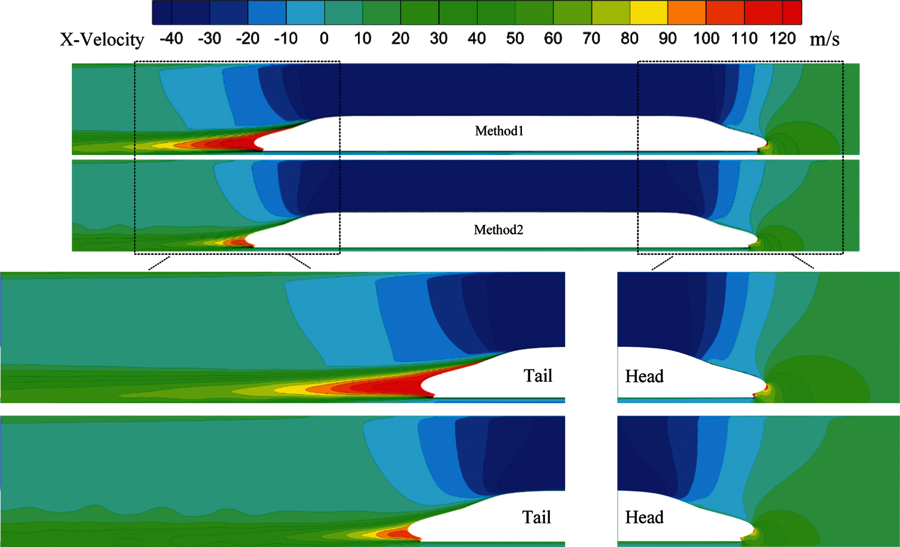
Figure 12: Time-averaged velocity around the train

The time-averaged vorticities around the train are shown in Fig. 13. It can be seen that the vorticity distributions of the high-speed train running in the tunnel for both methods are almost consistent. The high vorticity in the wake of the high-speed train is dominated by strips. Moreover, those regions are not continuous, and are connected by the weak vorticity regions. However, there are also differences in the vorticity amplitude of high-speed trains in the tunnel for the two calculation methods, mainly in the wake. The size and magnitude of the high vorticity calculated using Method 1 is obviously greater than that of Method 2.

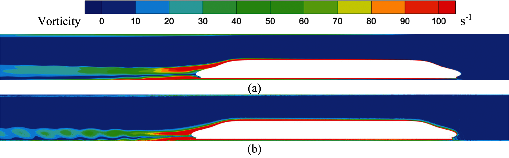
Figure 13: Time-averaged vorticity distribution around the train (a) Method 1 (b) Method 2

The vortex structures around the train are shown in Fig. 14. It can be seen that the two calculation methods have similar vortex structures when high-speed trains run in tunnels. When the high-speed air flows over the streamlined nose of the tail car, the airflow separates and then reattaches, with the separation producing a vortex street with opposite rotations. The moving distance of the vortex structure in the wake is very long. The main structure of the vortex is a worm-head worm. The flow around the high-speed train has similar vortex structure characteristics. However, the vortex structure scale and strength calculated using Method 1 are larger than those using Method 2.

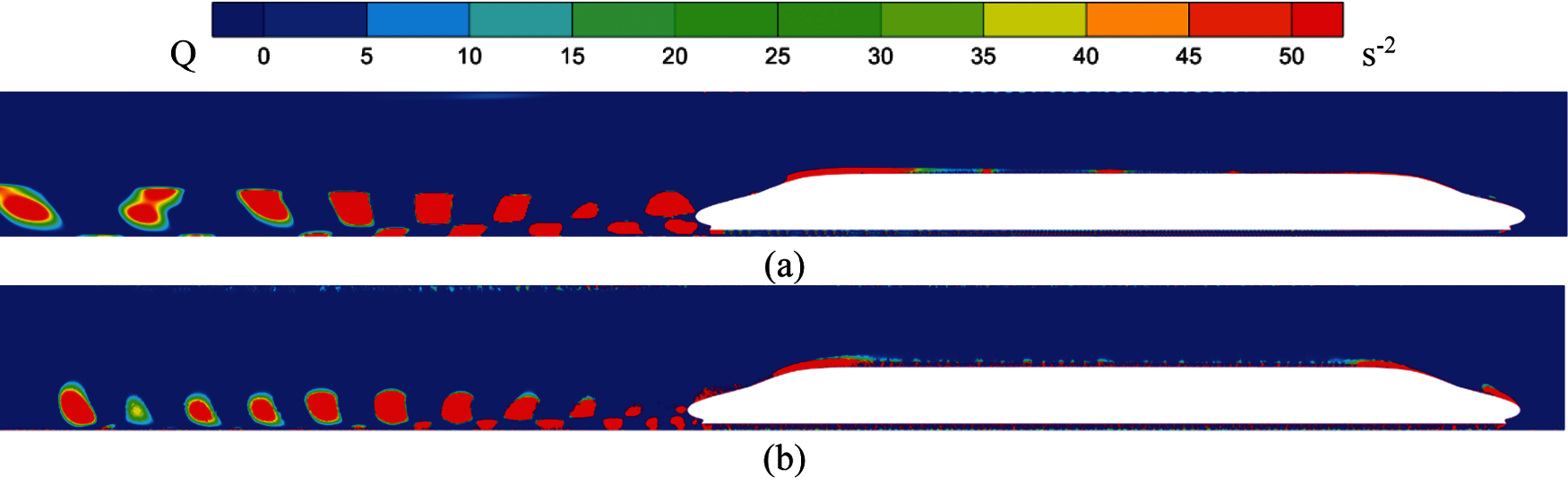
Figure 14: Spatial distribution of vortex structure (a) Method 1 (b) Method 2

4.3 Aerodynamic Noise Source

The intensity of the dipole noise source can be characterized by the root mean square of the time gradient of the fluctuating pressure on the train surface. According to the intensity of the fluctuating pressure on the train surface, the sound power level of the train surface can be found, as shown in Fig. 15. The sound power level distribution trends on the surface of high-speed trains for both methods are almost consistent. There is a slight difference in the sound power level on the streamlined surface of the tail car and the upper surface of the train. The surface sound power level of the train calculated using Method 1 is larger than that of Method 2.

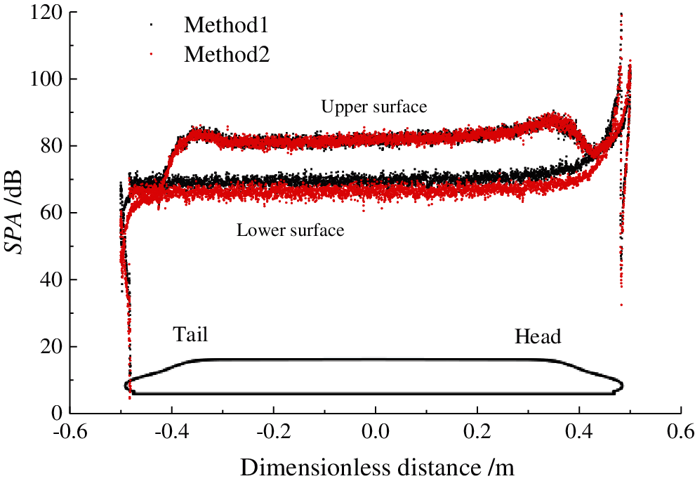
Figure 15: Sound power level on the surface of the train

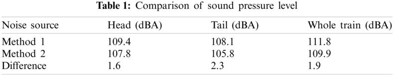
The aerodynamic noises generated by the head and tail cars are calculated. The fluctuating pressure on the train surface within 0.5 s of the sound source data is extracted. Then, the sound pressure at the noise evaluation point R1 (position shown in Fig. 1) is calculated using the acoustic integral formula [33]. For Method 1, the position of the noise measuring point is fixed, whereas the moving noise measuring point is used for Method 2, with its position relative to the train being unchanged. Fig. 16 shows the 1/3 octave frequency distribution of R1 noise measurement points. The aerodynamic noises of both head and tail cars show consistent trends for the two different methods. The main noise energy of the train is concentrated in the wide frequency range of 500 to 4000 Hz. Table 1 shows the contribution of the head and tail to the total noise, obtained by different calculation methods. From the table, the total sound pressure levels of the measuring points, obtained using Method 1 and Method 2 are 111.8 and 109.9 dBA, respectively. The sound pressure level calculated using Method 1 is 1.9 dBA larger than that found using Method 2. The head has a greater contribution to the total sound pressure level. Taking the head or tail as the aerodynamic noise source, the differences in sound pressure level obtained by the two calculation methods are 1.6 and 2.3 dBA, respectively.

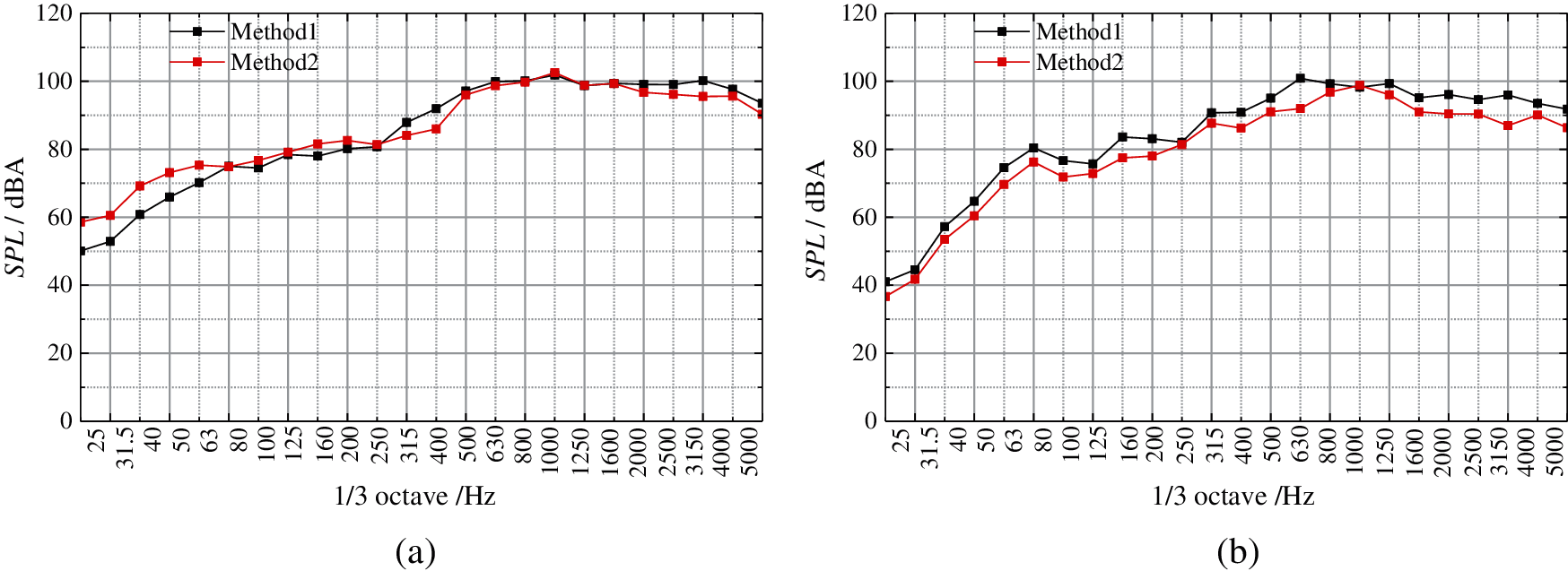
Figure 16: 1/3 octave frequency comparison (a) Head car (b) Tail car

The computational time spent by the two numerical calculation methods were recorded. The computational time using Method 1 is about 1/4 of that for Method 2.

5  Conclusions

Two different numerical methods are used to obtain the flow around and aerodynamic noise source of a high-speed train running in a tunnel. Method 1 is based on the principle of relative motion, whereas Method 2 uses a dynamic mesh, combined with adaptive mesh method. By comparing the train surface pressure, flow field structure and aerodynamic noise source characteristics obtained using the two methods, the following conclusions can be drawn.

(1)   When high-speed trains run in tunnels at speeds below 0.3 Ma, both methods provide similar flow field, train surface pressure and aerodynamic noise source results. The result obtained using Method 1 is slightly larger than that found using Method 2 in the terms of the magnitude of the surface pressure on the tail car, the size and intensity of the vortex in the wake, and the intensity of the noise source.

(2)   Both methods can effectively simulate the flow around and the aerodynamic noise source of the high-speed train, running in the tunnel. The difference in the sound pressure level between the two methods at the same noise measurement point is less than 2 dBA. Compared with Method 2, Method 1 has a higher efficiency and is more suitable for engineering applications.

Funding Statement: This work is supported by the National Key Research and Development Program of China (2020YFA0710902), Sichuan Science and Technology Program (2021YFG0214, 2019YJ0227), Fundamental Research Funds for the Central Universities (2682021ZTPY124) and State Key Laboratory of Traction Power (2019TPL_T02).

Conflicts of Interest: The authors declare that they have no conflicts of interest to report regarding the present study.

This work is licensed under a Creative Commons Attribution 4.0 International License, which permits unrestricted use, distribution, and reproduction in any medium, provided the original work is properly cited.