Computer Modeling in Engineering & Sciences

DOI: 10.32604/cmes.2022.018313

ARTICLE

Deep Learning-Based Algorithm for Multi-Type Defects Detection in Solar Cells with Aerial EL Images for Photovoltaic Plants

Wuqin Tang, Qiang Yang and Wenjun Yan*

College of Electrical Engineering, Zhejiang University, Hangzhou, 310027, China
*Corresponding Author: Wenjun Yan. Email: yanwenjun@zju.edu.cn
Received: 15 July 2021; Accepted: 15 October 2021

1  Introduction

In the past decades, the huge capacity of solar energy has been established around the world and the energy conversion efficiency of photovoltaic (PV) has achieved tremendous improvements year by year [1,2]. However, the conversion efficiencies can be impaired due to the long-time exposure under outdoor conditions that can cause long-term deterioration of PV module performance [3,4]. To detect the defects in the PV module, several physical algorithms are proposed. For example, current-voltage (IV) characteristics have been widely used to evaluate the status of the PV module [5–7]. However, IV curves could be scarcely influenced by some tiny defects that make it infeasible to accurately detect defects in PV modules [8]. In addition, infrared (IR) imaging is employed to detect the defects. The idea behind the IR imaging is that the temperature in the defective area is higher than the normal area. However, such a technique cannot detect micro-defects due to the low resolution of IR images [9].

The inner structure of a silicon PV module is presented in Fig. 1. The current generated in a cell is collected and transferred through the busbars. The power generated in a PV module is the sum of all cells in the module. Therefore, the cell is a basic unit of a PV module and almost all of the defects in EL images are cell-level.

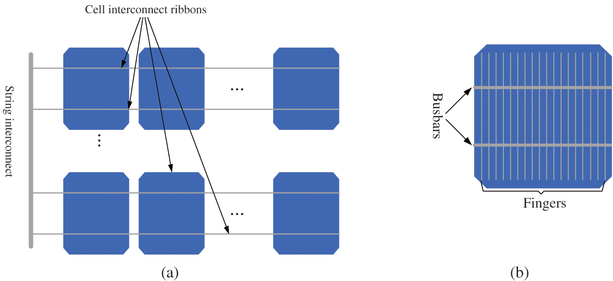
Figure 1: Inner structure of PV module and cell: (a) strings; (b) a cell

In recent years, EL is treated as an excellent technique to detect defects in PV modules. The idea behind it is that when a specified current is injected into the PV module, radiative recombination of carriers can create light emission and the light can be collected by the specified camera. Therefore, EL images can provide an inner perspective to evaluate the state of PV modules [10,11]. Given that the PV plants are always deployed in remote areas covering a large geographical area or some unsuitable places for human operation, the manual inspection with EL images is unfeasible, especially for large-scale PV plants. A set of studies for automatic defect detection using EL images has been carried out as follows. In [12], a series of image processing algorithms are proposed to extract cells from the PV module and then a well-trained CNN is used to recognize the crack. In [13], a public dataset of solar cells is provided that contains 2,624 solar cell images and two approaches are proposed to classify the EL images. In [14], a fusion model of Faster R-CNN and R-FCN is proposed to detect solar cell surface defects. In [15], an efficient method for defects inspection has been proposed that leverages the multi-attention network and the hybrid loss to improve the performance. In [16], a pipeline is developed to extract and classify the cell from the PV module. In [17], a deep learning-based defect detection of a photovoltaic module is proposed and GAN is introduced for the data augmentation. In [18], a novel complementary attention network is introduced that suppresses the noise feature in the background and enlarges the defects features simultaneously. In [19], a model is proposed to predict PV module electrical properties from EL image features using pixel intensity-based and machine learning-based classification algorithms. In [20], the detection of a crack in the PV module manufacturing system is presented and the proposed solution can identify the cells with cracks with high accuracy. In [21], the effect of crack distributions over a solar cell in terms of output power, short-circuit current density and open-circuit voltage was investigated. In [22], a new architecture that integrated fuzzy logic and convolution operations was proposed to suppress the subjectivity and fuzziness of defects recognition. In [23], an encoder-decoder network is proposed to perform semantic segmentation of EL images. In [24], a deep learning-based detection of multi-type defects was proposed to implement inspection in the production line. In [25], a deep feature-based method was proposed to classify the defects. In this paper, the deep features were extracted by deep neural networks that were classified with machine learning methods.

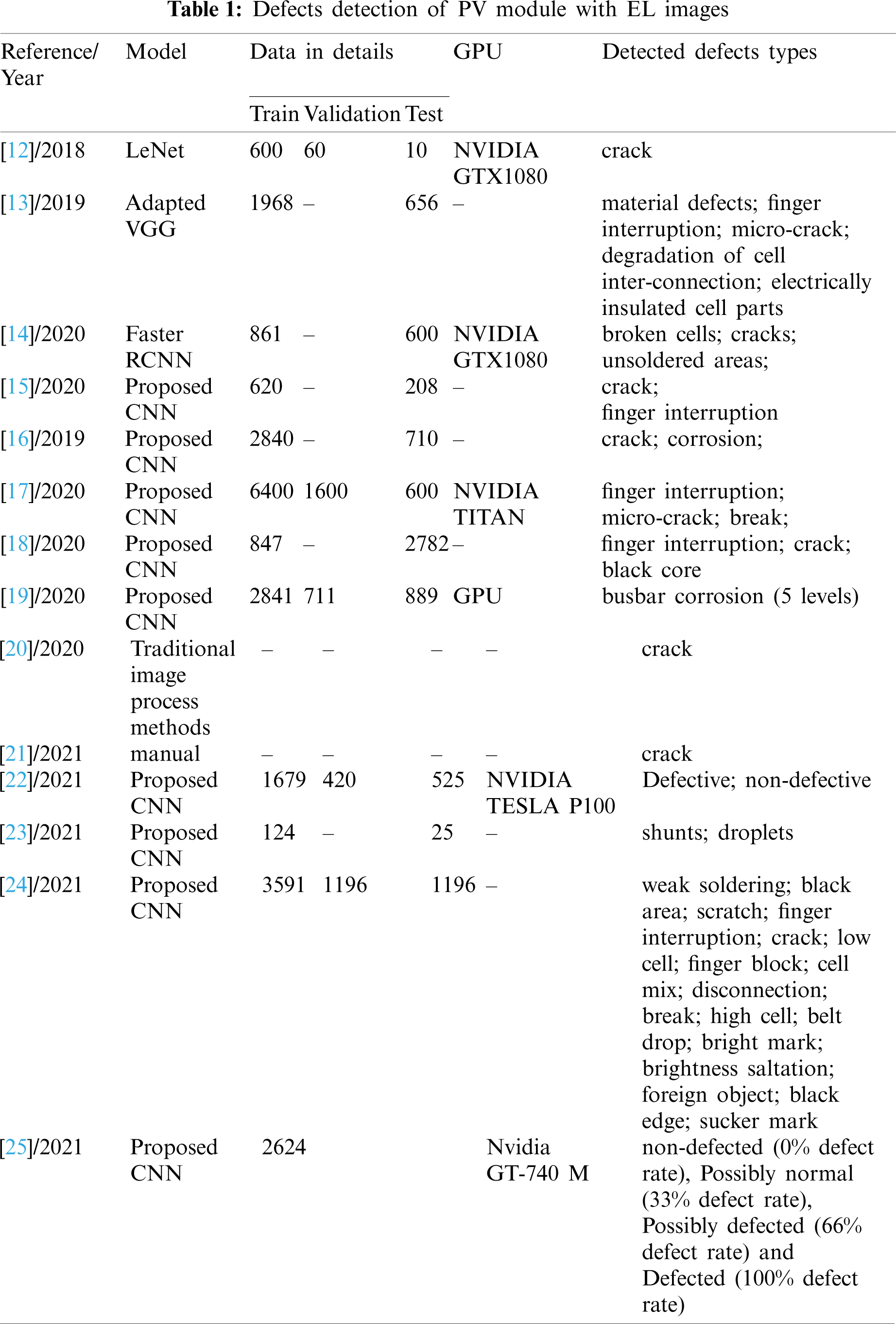
The details of the previous work [12–25] are presented in Table 1. The limitations of these solutions can be summarized as follows: (1) Most images used in the previous studies are collected during the factory inspection and the resolution of the images captured during the factory inspection is generally much higher than those collected during the field inspection using the unmanned aerial vehicle (UAV). The solution used in the references could not be appropriate for the field inspection; (2) The dataset with sufficient images covering all defects can be hardly obtained, and the unknown or unlabeled defects may exist in the original dataset. This can degrade the defect detection performance; (3) Image annotation for the unknown or unlabeled defects can be time-consuming in practice. These limitations may significantly degrade the performance of automatic defect detection using EL images in terms of both efficiency and accuracy in large-scale photovoltaic plants.

To address the aforementioned challenges, a novel approach using the combination of deep learning, deep clustering, and transfer learning is introduced to establish our defects detection system of PV cells with EL image, which can recognize the labeled and unknown or unlabeled defects with high performance. Specifically, a deep learning-based features extractor and classifier are proposed to extract the deep features of images and classify the images. In addition, a deep clustering with unsupervised manner is designed to automatically classify the unlabeled or unknown defects. The structure of the CNN is adapted to improve computing efficiency. The framework of the proposed algorithmic solution is illustrated in Fig. 2.

The proposed defects detection system utilizes the phased design to address the outstanding technical challenges from both algorithm and system perspectives. The technical contributions made in this work are as follows:

1)   A deep clustering algorithm is designed to cluster the different unknown or unlabeled defects based on the distance difference of the defects feature vector that is extracted by the well-trained CNN-based model. In addition, the deep clustering algorithm can be classified in an unsupervised manner;

2)   A transfer learning algorithm is introduced to accurately detect the newly formed defects that are classified by the deep clustering algorithm. Data augmentation is applied to increase the performance of the CNN-based classification model;

3)   To get the best trade-off between the performance and computing complexity, the effect of the model structure is considered and analyzed. The proposed model can obtain high accuracy with relatively simple computational complexity;

4)   A real-world testbed with unmanned aerial vehicles (UAV) is built. To the best of the authors’ knowledge, this work is the pioneering work to adopt the UAV for EL inspection in PV plants. In addition, a data set of EL images of PV modules with various defects is well established and maintained. The EL image can be shared when requested for non-commercial purposes.

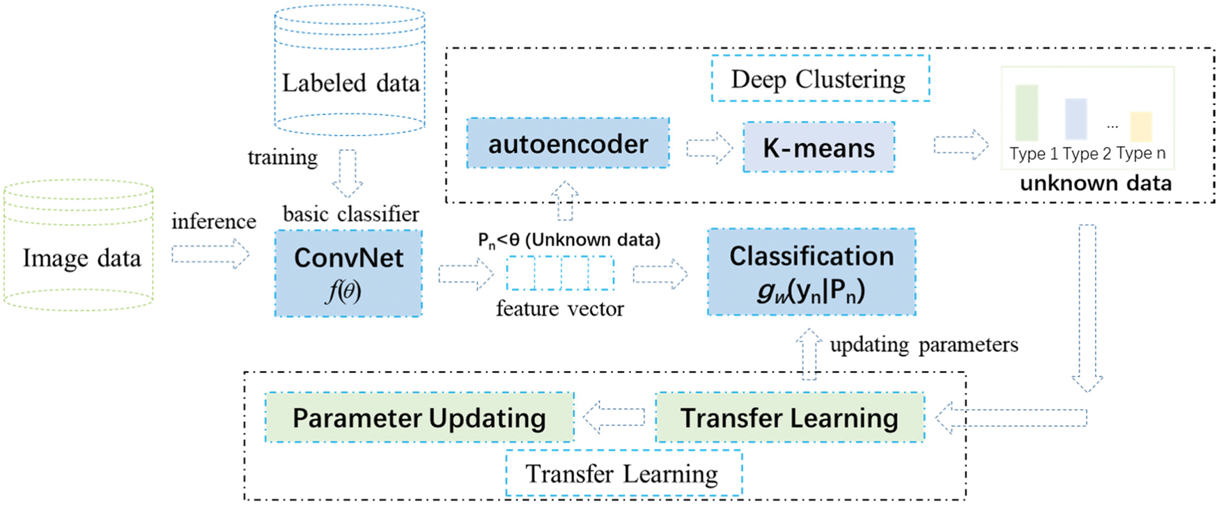
Figure 2: Framework of the proposed defect detection algorithm

The remainder of the paper is organized as follows: Section 2 presents the details of the proposed algorithm; In Section 3, the performance of the proposed solution is evaluated through extensive experiments and the numerical results are presented and discussed; finally, the conclusive remarks and future work are given in Section 4.

2  The Algorithm for Defects Detection

The framework contains several parts and steps that are presented in Fig. 3 and the crucial parts are simply illustrated as follows:

The feature extractor (ConvNet f(θ)): The extractor is a refined CNN-based model to extract the feature vectors for defects classification or clustering. In the pre-training process, the classifier is firstly trained and obtains the original parameters with the original labeled images. To reduce the computational complexity, the parameters in ConvNet are frozen in the transfer learning period. The augmentation of the images is introduced to further improve the system performance.

Classifier (gw(yn|Pn)): The classifier is a fully connected layer to classify the defects. In the pre-training period, gw can get the initial parameter to distinguish the original labeled images and in the transfer learning process, the parameter in gw is updated to classify the novel dataset. To increase the performance, the augmentation of the images is also introduced.

Unknown defects detector: Given that several defects in the collected dataset are unknown, we introduce a deep clustering algorithm to recognize the unknown defects without human intervention. A threshold ξ is used to distinguish the unknown defects. An autoencoder and k-means algorithms are designed to classify the unknown defects.

Transfer learning and updating strategy: To decrease the computing consumption, transfer learning is introduced to learn the feature of newly defects classified and the images with unknown defects can be classified automatically and transfer into the training set.

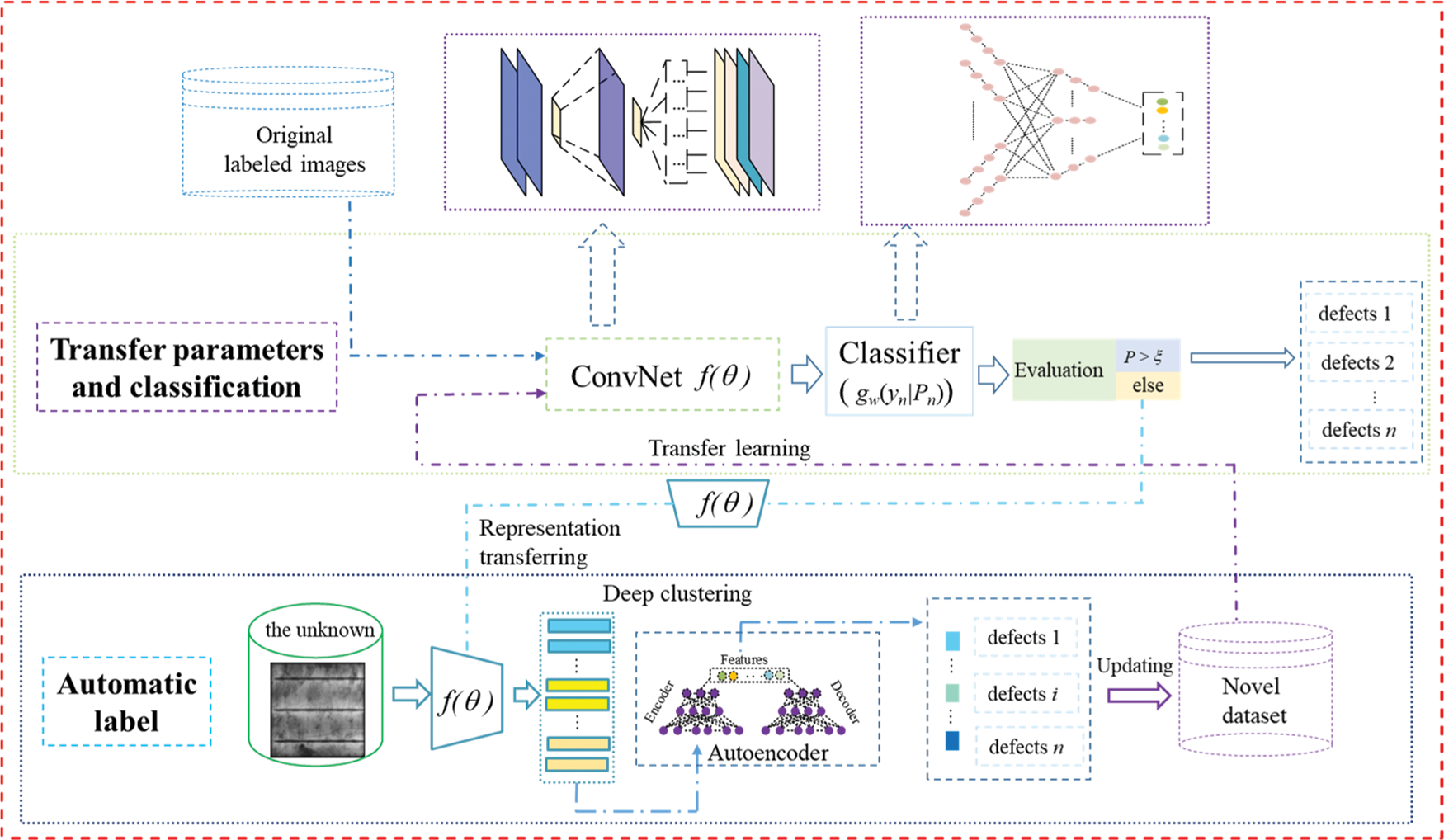
Figure 3: Details of the proposed defect detection algorithm

The details of the above algorithms are illustrated as follows.

2.1 The ConvNet and Defects Classifier

The aerial images of PV cells in the collected data set are represented as \{{(I1, p1), (I2, p2),…, (In, pn)}\}, where Im is the images collected at the mission point m. The images in the training set are denoted as T= \{{(x1, y1), (x2, y2),…, (xn, yn)}\}, where xm means the mth images in the training set and ym is the class label of the mth images.

Motivated by [17], a novel structure of the deep learning-based model is proposed to extract the feature or representation of the image. The model for features extraction is denoted as ConvNet that contains two blocks: block A and block B and the classifier contains two fully connected layers. The structures of blocks A and B in ConvNet and the classifier are presented in Figs. 4a--c, respectively.

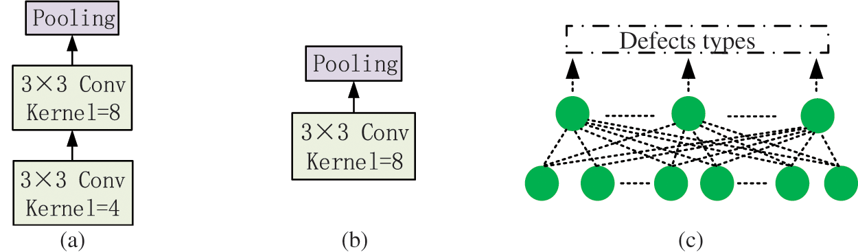
Figure 4: The structure of ConvNet and classifier: (a) block A in ConvNet; (b) block B ConvNet; (c) classifier gw

In fact, the deep learning-based model can be considered as a ConvNet mapping (f(θ)), where θ is the parameters in the mapping. The vector obtained by applying the mapping is the representation or feature of the input image. To classify the image, a parametrized classifier gw is built on the top of the ConvNet f(θ), where w is the parameter of the classifier. The label predicted by gw is the image's types to one of the k possible pre-defined classes. The purpose of the training process in the training set is to find the parameters θ∗ and w* that the f(θ∗) and gw∗ can get the good general features and recognize the defects with high accuracy. The parameters θ and w are jointly updated by optimizing the following issue:

minθ,w⁡(∑jl(gw(fθ(xj)),yj))(1)

where l is the cross-entropy loss function that is commonly applied to the classification task, as presented in (2):

E=−∑jtklog⁡(yk)(2)

where yk is the output of the deep learning-based model and tk is the label of the image. The loss function is minimized by the mini-batch stochastic gradient descent. The output of a layer in the model can be computed as follows:

xl=f(ul),withul=Wl⋅xl−1+bl(3)

where xl is the output of the lth layer and Wl and bl is the weight and bias in the lth layer. The updating of the weights can be calculated by (4) and (5)

Wijl=Wijl−1−η∂E∂Wijl+νijl(4)

vijl=γvijl−1−ληwijl−1(5)

where ∂E∂Wijl is the gradient of the kernel weights and η is the learning rate, Wijl and vijl denote the weight and momentum between the neuron i in lth layer and the neuron j in (l+1)th layer.

To improve the performance of the proposed model, data augmentation is widely applied to increase the size of the data. It has been proved in [17,25] that generative adversarial networks can create synthetic images and improve the performance of the deep learning-based method. However, due to the operation complexity of GANs and the size of the collected EL images data, Gaussian blur and geometric transformation are performed in this paper to increase the number of training samples. The details of our data augmentation algorithm are presented in Algorithm 1.

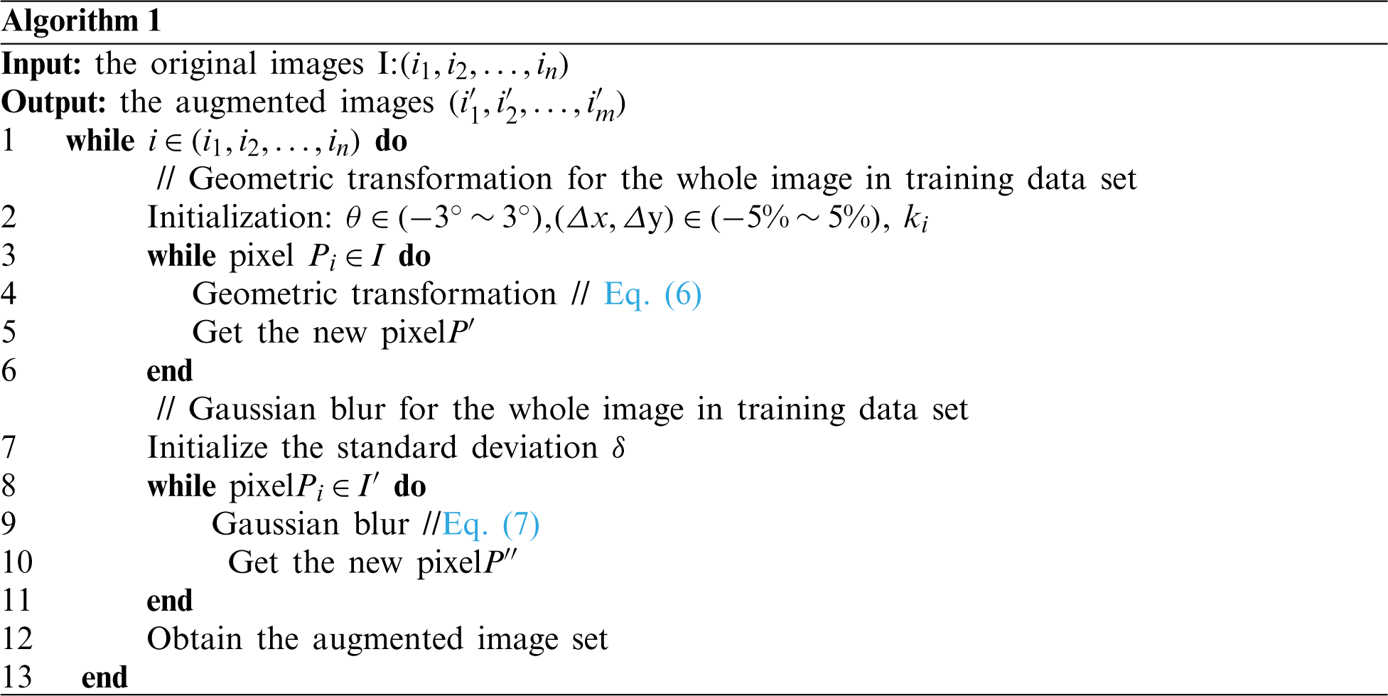
The grey value in the point (x, y) of image i is denoted as Pi(x, y) and the corresponding transformed grey value is denoted as Pi′(x,y). The geometric transformation can be performed by (6)

{x′=kx1⋅x⋅cos⁡θ+ky1⋅y⋅sin⁡θ+Δxy′=ky2⋅y⋅cos⁡θ−kx2⋅x⋅sin⁡θ+Δy(6)

where θ∈(−3∘∼3∘) is the rotation angle, kx1∼2, ky1∼2 are the transformation coefficients and (Δx,Δy)∈(−5 are the translation factors in axes x and y. The operation of Gaussian blur can be performed by (7)

Pi(x′,y′)=Pi(x,y)⋅G(x,y)=Pi(x,y)⋅12πδ2⋅e−(x2+y2)/2δ2(7)

where G(x, y) is the Gaussian function and δ is the standard deviation.

2.2 Unknown Defects Recognition and Training Set Upgrade Strategy

The images of PV cells captured by UAV are denoted as χ: (x1, x2,…,xn) and all χ: (x1, x2,…,xn) are transferred into the well-trained classifier that is described in Section 2.1. The well-trained classifier is represented by gw(f(θ)) and the output of the classifier is the marginal probability distribution P. Therefore, the classification of a PV cell can be denoted as \{{xi, yi, Pi}\}, where xi is an image of PV cell, Pi is the maximum probability of the predicted label yi.

If the output of classifier Pi <ξ, where ξ is the preset threshold, it is reasonable to believe that xi is an unknown defect. To classify the same type of unknown defects, a deep clustering algorithm (DC) is designed.

The proposed deep clustering algorithm contains two parts: (1) autoencoder; (2) k-means algorithms. The autoencoder is to extract the dominant features and consists of an encoder and decoder. The autoencoder is trained to minimize the reconstruction error, which is presented in (8)

l(z,z′)=||z−z′||2(8)

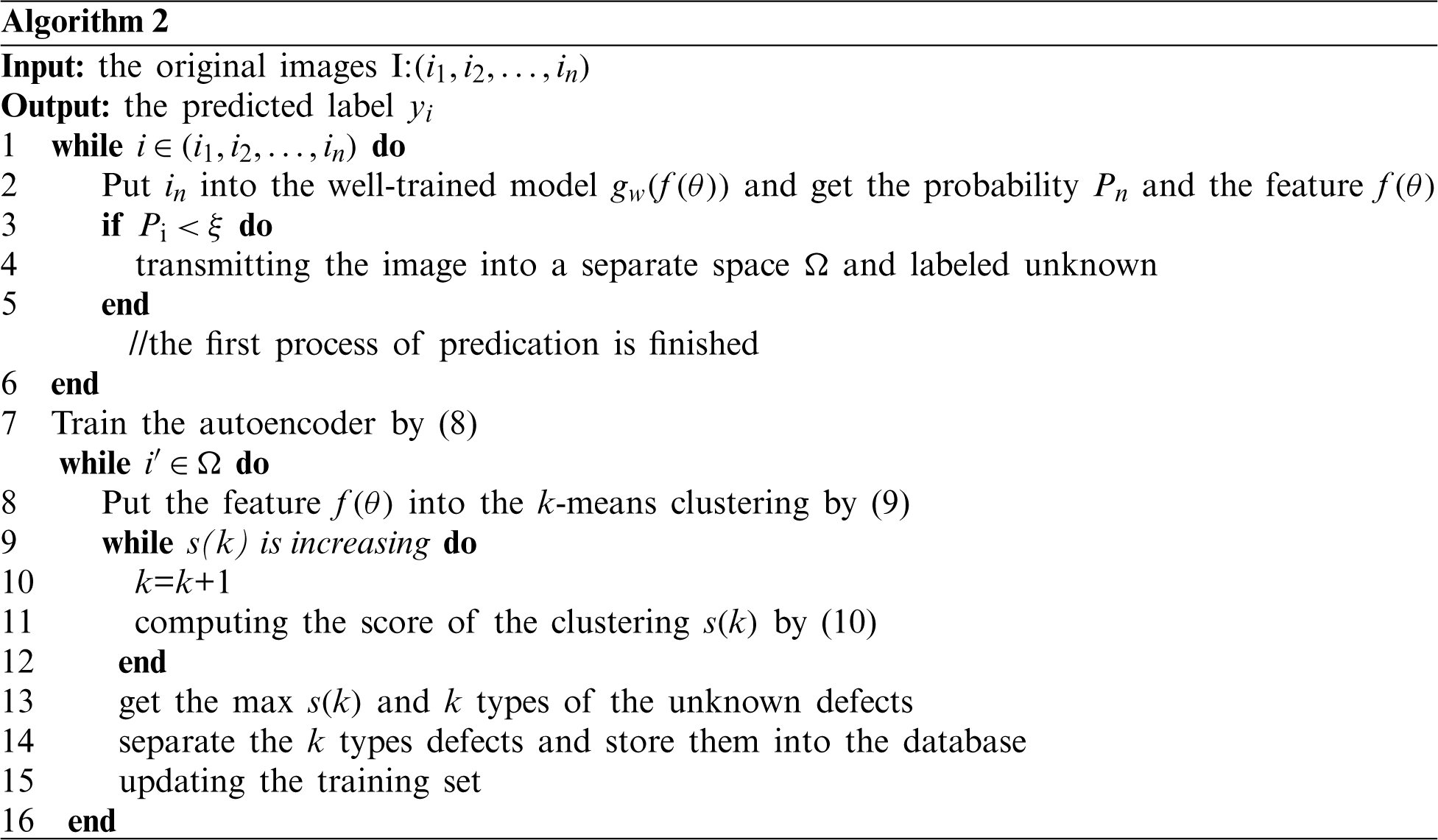
Preliminary research [26] indicates the choice of the clustering algorithm is not crucial and in this paper, we introduce a standard clustering algorithm, k-means, to group the features extracted by ConvNet. In our cases, the features fθ(xn) computed by ConvNet are clustered into k groups. More specifically, k-means for the features is to minimize the within-cluster k square as presented in (9)

min∑j=1k∑z∈Si||z−ui||(9)

where ui is the arithmetical mean of points in the nearest or same center set Si. The pseudocode of defect detector and training set updating strategy is presented in Algorithm 2.

s(k) is introduced to calculate k, as given in (9). More specifically, in (10), a smaller Wk and larger Bk indicate higher s(k), and hence a better clustering performance. Therefore, when max s(k) is obtained, k can be calculated.

s(k)=tr(Bk)tr(Wk)⋅m−kk−1(10)

where Bk is the trace of the between group dispersion matrix and Wk is the covariance matrix of data in the same type, and tr is the trace of the matrix.

2.3 Detection of the Unknown Defects Using Transfer Learning

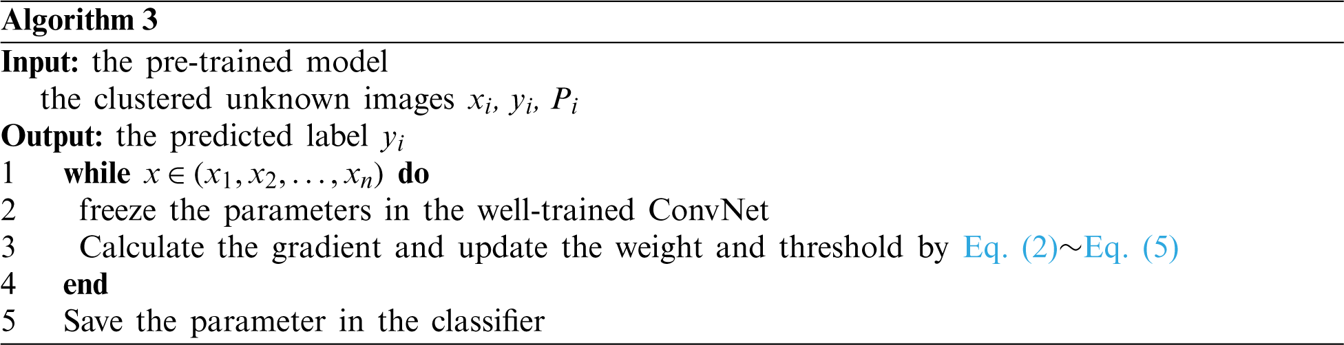
To decrease the computing complexity, transfer learning is introduced to train the classification model. In this paper, the labeled training set is considered as the source domain Ds={χ,P(X)}, where χ is the feature space of the labeled PV cell images and P(x) is marginal probability. Similarly, the target domain can be denoted as T=(x,f(⋅)), where x is the feature space in the target domain and f(⋅) is the target predictive function. The purpose of our design is to improve the learning process of predictive function f(⋅) using the knowledge in Ds.

The earlier layers in the deep learning-based model are to extract the generic features from images, e.g., colors, edges and shapes, while the deeper layers are more likely to learn the more abstract features for classification [27]. Depending on the defects features in the EL images, it is optional to fine-tune the last full connected (FC) layer in the classifier and freeze the earlier layer in the ConvNet. ConvNet is used as the feature extractor for the image representation that is pre-trained on the given training set.

In the training process, the Adam optimizer is used for backpropagation and the categorical cross-entropy is used as the loss function that is presented in Eq. (2). The details of the process are described in Algorithm 3. In this paper, the classifier is presented in Fig. 4c.

3  Experimental Assessment and Numerical Results

In this section, numerical experiments have been performed to evaluate the performance of the proposed algorithms. In this paper, the collected paper contains EL images with several types of cell conditions: good condition, crack, finger interruption, black core, busbars corrosion, which is presented in Fig. 5.

The data set is collected with a UAV-based platform in the real PV plants in Gonghe, Qinghai Province, China (100 MW). The platform is presented in Fig. 6. In the platform, four-rotor aircraft, DJI M300 is employed and some others accessories to establish the platform contain EL camera, X-port and Manfold2. In addition, a high-performance computation platform (with 4 NVIDIA TITAN GPUs) is used to decrease the computing time during the training process. The installed software for implementing the computing are Python and Pytorch.

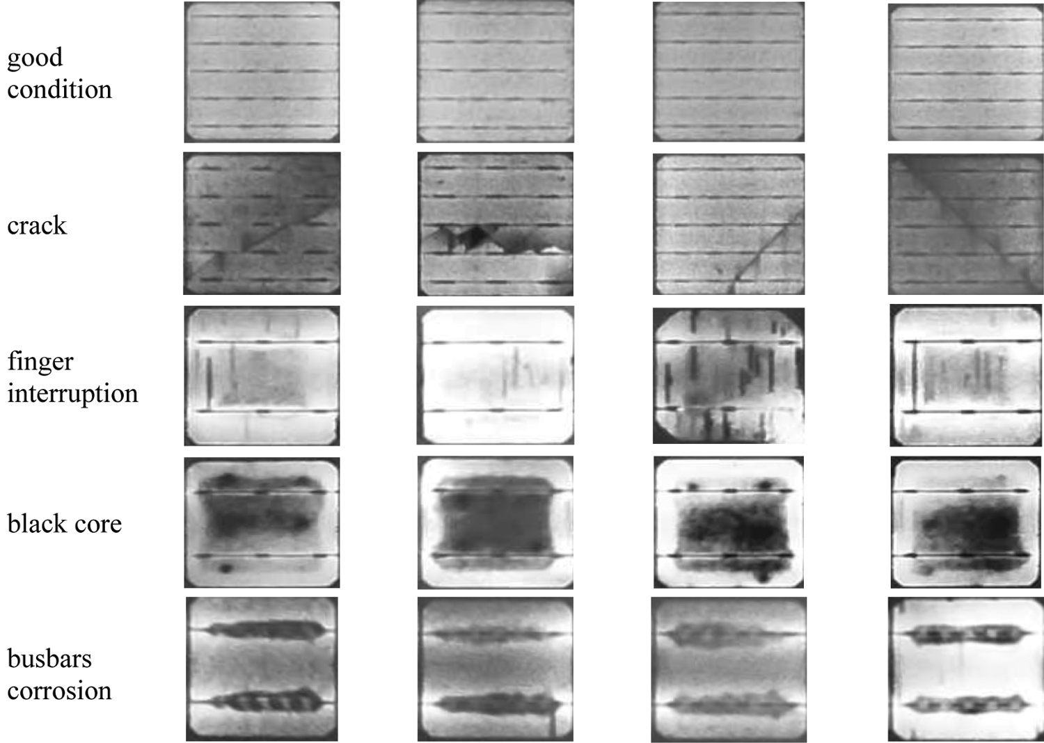
Figure 5: Sample images of PV cells in different conditions

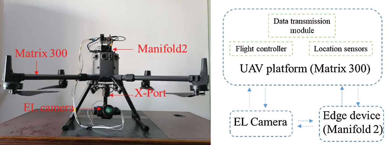
Figure 6: The UAV-based platform

3.1 Effects of the Models Using Different Structures

In this section, we evaluate the effects of the model with different structures. As mentioned previously, the features extracted from earlier layers in the deep learning-based model could include more information about color, edge or texture and the features extracted by the deeper layer can be more abstract. The experiments are carried out to evaluate the performance of these models with different structures and parameters, and the numerical results are presented in Fig. 7. Here, in total five models, i.e., (c1p1), (c1c2p1), (c1c2p1c3p2), (c1c2p1c3c4p2) and (c1c2p1c3c4c5p2), are extensively compared and analyzed. These models are represented by Model 1∼Model 5, where (ci) and (pi) are the ith convolution layers and the ith pooling layer, respectively. At the end of the model, two fully connected layers are adopted to classify the defects. In addition, given that the feature mappings extracted by different kernels can be different, the impact of the kernel (k = 2, 4, 8, 16) in the convolution layer is also analyzed.

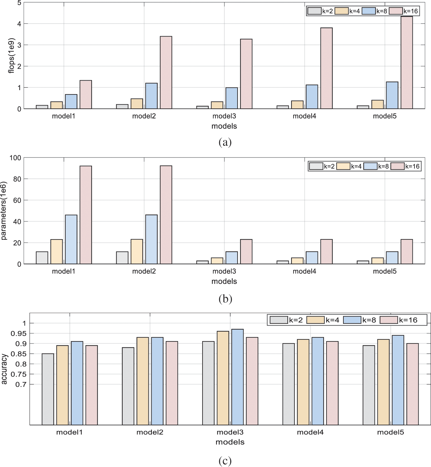
Figure 7: Experimental evaluation of CNN model with different parameter settings: (a) flops of different models; (b) parameters of different models; (c) mean accuracy of defect detection

It can be inferred from Figs. 7a and b that with the increasing of the kernel number, the parameters and flops grow rapidly. It means that the computing process has become more complicated along with the increase of kernel number. When the number of kernels is doubled, the parameters and flops are about doubled. The results presented in Fig. 7c illustrate that the growth of the number of kernels from 2 to 8 can increase the accuracy because more kernels can provide more deep features. However, we also noticed that when the number of kernels is beyond 8, the performance could be damaged. It is indicated that the convolution layer with 4 or 8 kernels is sufficient to extract the defects features in EL images. In addition, an additional number of kernels could increase the computing complexity greatly. Therefore, model 3 is selected to classify the defects.

3.2 Performance of Classification Accuracy and Implementation Details

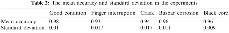
In this section, we trained the proposed deep learning-based model for 160 epochs. Once the training process is completed, the parameters with the lowest validation loss are loaded to the model for test. To evaluate the performance of the proposed solution, a 10-fold cross-validation scheme is introduced. The original dataset, which contains 5,000 EL images (1,000 images for each type of condition), is equally divided into ten parts and each part contains 100 images for each type of condition. In the experiment, seven parts, two parts and one part are selected randomly as the training, validation and test set. The mean accuracy and standard deviation for each type are presented in Table 2.

To show the performance of the proposed methods, the confusion matrix is presented in Fig. 8.

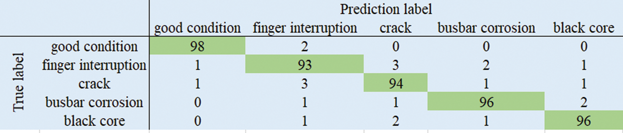
Figure 8: Classification confusion matrix

The classification accuracy of different defects is presented in Table 2. The classification accuracy of the proposed model is all beyond 0.9 and the mean accuracy of defects classification in the 10-fold cross-validation scheme is 0.95. The accuracy of finger interruption is the lowest (0.93). This is due to that some features of finger interruption could be covered by the background.

To analyze the features extraction ability of the proposed model, class activation maps (CAM) are introduced to visualize the learned features [28]. For easy explanation, the feature map of the top convolution layer is used as the input to create the heat map. Fig. 9 shows the visualization of the extracted features map. It can be concluded from Fig. 9 that the proposed model can extract the defects feature with high performance.

3.3 Performance of Unknown Defects Detector

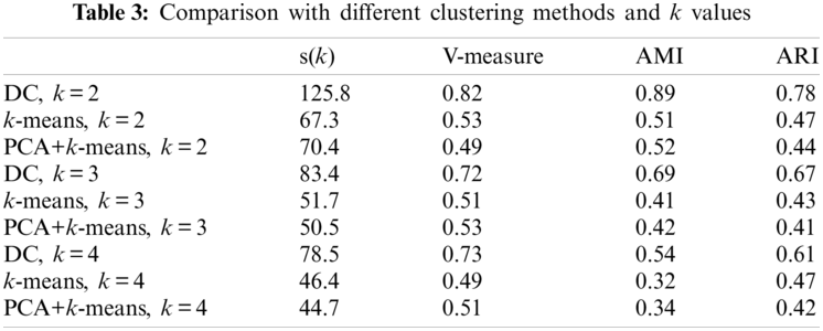
In this part, the proposed deep clustering method is evaluated with the existing methods. In the experiments, crack and finger interruption are treated as the known defects as well as the cells in good condition, while busbars corrosion and black core are considered as the unknown defects. 2,400 images (about 800 images in each labeled type) are used to train the ConvNet and 200 images of the cells with busbars corrosion and black core are used to test the deep clustering. The pre-trained ConvNet is used to extract the 256-D features from the input images. Then, k-means is employed to separate the features extracted from the unknown images and k can be determined by Eq. (10). All the hyperparameters in the models are set randomly and the learning rate is 0.0001. In Table 2, scores of the proposed deep clustering (DC) with different k values are obtained. It can be observed that the highest score is calculated when k is 2, which matches the experiment setup.

Figure 9: Visualization of the feature mappings

To evaluate the performance of DC, we introduce another two algorithms to implement the same task. One directly used k-means to cluster the images and another is called the combination of the principal component analysis with k-means (PCA+k-means) to cluster the original images. All the relevant settings in the experiments for the three methods are the same. Here, three commonly used metrics, i.e., V-measure, adjusted mutual information (AMI) and adjusted rand index (ARI), is introduced. The larger value of the metric indicates better performance. The results are all presented in Table 3 and it can be concluded that the proposed DC outperforms the other two benchmark methods in the three metrics most of the time. This is due to the fact that the direct k-means treat all the information as the same during the processing and the defects features could be covered by numerical noises, which can greatly impact the clustering results and although PCA+k-means can reduce the dimensionality of the features, PCA is not applicable to extract the features in EL image. In addition, the performance of the methods with the different number of clusters (k = 2, 3, 4) is presented in Table 3 and it can be observed that when k = 2, the best results are obtained, which matches the experimental setup.

3.4 Comparison with the Existing Methods

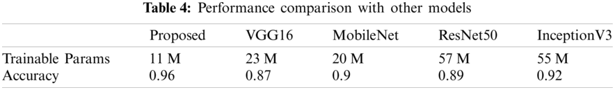
In this section, we compared the proposed method with the state-of-art approaches, namely, VGG16 [29], MobileNet [30], ResNet50 [31] and InceptionV3 [32]. To make these models more appropriate to the dataset, the last two layers in these models are replaced by two connected layers (1 × 1 × 256, 1 × 1 × 5). We do not change the other parameters in these models and the parameters are presented in [29–32].

In this work, accuracy, and trainable parameters in different models are considered and analyzed, which is presented in detail in Table 3. Those methods can extract the defects features with the combination of some convolution and fully connected layers. As presented in Table 4, the well-trained InceptionV3 can obtain a better accuracy of 92%, but the trainable parameters in the model are larger than the proposed method. Overall, the proposed method outperforms the above-mentioned models in the defect classification of EL images and provides the best trade-off between computational complexity and classification performance.

4  Conclusions and Future Work

This paper proposed a framework for the application of deep learning to address the problems of PV cells defects detection with EL images. A well-trained feature extractor (ConvNet) and classifier are obtained and given that there are some unknown defects during the inspection process, a deep clustering technique is proposed to distinguish the unknown or unlabeled defects without human intervention. To relieve the limitation of insufficient data, image augmentation is used. In addition, transfer learning is adopted to transfer the defects feature map to the target domain. The proposed algorithmic solution is evaluated extensively under different operational scenarios. The experiment results prove the accuracy and efficiency of the model.

For future work, the algorithms can be deployed in the edge devices for online defect detection and more types of defects types need to be considered and investigated. In addition, topological optimization can be introduced to obtain the best trade-off between computing accuracy and complexity.

Funding Statement: The authors received no specific funding for this study.

Conflicts of Interest: The authors declare that they have no conflicts of interest to report regarding the present study.

This work is licensed under a Creative Commons Attribution 4.0 International License, which permits unrestricted use, distribution, and reproduction in any medium, provided the original work is properly cited.