Computer Modeling in Engineering & Sciences

DOI: 10.32604/cmes.2022.018235

ARTICLE

The Method of Fundamental Solutions for Two-Dimensional Elastostatic Problems with Stress Concentration and Highly Anisotropic Materials

M. R. Hematiyan1,*, B. Jamshidi1 and M. Mohammadi2

1Department of Mechanical Engineering, Shiraz University, Shiraz, 71936, Iran
2Department of Mechanical Engineering, College of Engineering, Shiraz Branch, Islamic Azad University, Shiraz, 71993, Iran
*Corresponding Author: M. R. Hematiyan. Email: mhemat@shirazu.ac.ir
Received: 9 July 2021; Accepted: 8 October 2021

1  Introduction

The MFS is an integration-free meshfree method, which has found a wide application because of its accuracy and simplicity. In the MFS, the solution is expressed in terms of known fundamental solutions, which exactly satisfy the governing equations of the problem. This semi-analytic nature of the MFS makes it suitable for obtaining accurate solutions [1–3]. Meshfree methods can be classified into two major categories [4]. The first category includes meshfree methods based on strong forms of differential equations [5–7], while the meshfree methods based on weak forms of governing equations [8,9] fall into the second category. The weak-form meshfree methods need suitable techniques for the computation of domain integrals [10–12]; however, the MFS is a strong-form and truly meshfree method without any need for evaluating any domain or boundary integral. These features make the MFS suitable for problems with moving/unknown boundary [13 –15], for problems with concentrated loads [16–18], and moving load problems [19]. The boundary element method (BEM) is also a boundary-type method, which is based on the fundamental solutions of the problem, as in the MFS, and results in accurate solutions. The BEM needs special techniques for the evaluation of singular [20,21] and nearly singular [22,23] domain/boundary integrals; however, the MFS is an integration-free method.

The literature review shows a few studies on the MFS for the analysis of elastostatic problems in anisotropic media. Raamachandran et al. [24] made use of the charge simulation method, which is the same as the MFS. They solved some anisotropic elastostatic problems and obtained satisfactory results. Berger et al. [25] presented a domain decomposition MFS for deformation analysis of bimaterial anisotropic bodies and showed that the MFS could result in accurate solutions. Tsai [26] used the MFS for solving three-dimensional elastostatic problems in transversely isotropic media. He proposed a rescaling method for improving the accuracy of the results of problems with natural boundary conditions. Recently, Hematiyan et al. [27] presented the MFS for anisotropic thermoelasticy in 2D media and showed that the MFS results in accurate solutions.

Other variants of the MFS have also been used for anisotropic elasticity. Liu et al. [28] employed the non-singular MFS for the deformation analysis of 2D anisotropic media with one or two materials. In the non-singular MFS, a fictitious source (force) distributed over a circle is used instead of a concentrated singular source. Recently, Liu et al. [29] proposed the localized MFS (LMFS) for solving 2D anisotropic elastostatic problems. Some boundary as well as interior collocation points should be considered in the LMFS. The LMFS can be more efficient than the MFS for large-scale problems [30].

Base on the above literature review, it can be seen that the MFS and its variants have been employed for solving anisotropic elastostatic problems; however, the parameters, which have significant influence on the accuray of the MFS for solving these problems, have not been studied yet. In this work, influences of three important parameters, i.e., the degree of anisotropy of the problem, the ratio of the number of collocation points to the number of source points, and the distance between main and pseudo boundarires, on the accuracy of the MFS results are numerically investigated. Determining a suitable configuration of source points is a major issue in the MFS. There are many studies on the location of source points and collocation points in the MFS. Among them, one can refere to the works on Laplace and Helmholtz equations [1,31–35], biharmonic equation [36,37], torsion problem [38], transient heat conduction [39], and isotropic elasticity [40–42]. Yet, no research has been carried out on the configuration of source points for anisotopic elasticity.

2  The MFS Formulation for Two-Dimensional Anisotropic Elasticity

Consider a plane stress/strain problem in the anisotropic domain Ω, whose boundary is denoted by ∂Ω. The variation of the stress components σxx, σyy, and τxy (σ11, σ22, and σ12) in the domain can be expressed by the equilibrium equations as follows [43]:

∂σxx∂x+∂τxy∂y=0,in Ω, (1)

∂τxy∂x+∂σyy∂y=0,in Ω. (2)

Representing the displacement components in the x and y (x1 and x2) directions by u and v (u1 and u2), respectively, the strain components can be expressed as follows [43]:

εxx=∂u∂x,εyy=∂v∂y,2εxy=∂u∂y+∂v∂x. (3)

The relationship between strain and stress components can be written as follows:

[εxxεyy2εxy]=[a11a12a16a21a22a26a61a62a66][σxxσyyτxy], (4)

where aij are the elastic compliance coefficients of a monoclinic material. In 2D anisotropic elastostatic problems, the material possesses a plane of material symmetry, and the out-of-plane and in-plane deformations are decoupled. This work deals with monoclinic materials; however, because of the wide applications of orthotropic materials, the relationship between conventional elastic constants of orthotropic materials and the corresponding compliance coefficients are also described. An orthotropic material has three mutually perpendicular planes of symmetry. For an orthotropic material with material directions in x and y directions, we can write [43]:

a22=S22,a26=a62=0,a66=S66. (5)

for plane stress problems, and

a22=S22−S232S33,a26=a62=0,a66=S66. (6)

for plane strain problems. The constants Sij in Eqs. (5) and (6) are expressed as follows:

S12=−ν21/E2=−ν12/E1,S13=−ν31/E3=−ν13/E1,S23=−ν32/E3=−ν23/E2. (7)

Ei represents the Young’s modulus in the xi direction. μij and νij are respectively the shear modulus and the Poisson’s ratio in the xixj plane. If the principal material directions of the orthotropic material make an angle with x and y directions, the elastic constants aij can be found by a transformation. The transformation is described in Appendix A.

In plane stress/strain problems, two boundary conditions are considered for a boundary point that can be expressed as follows:

L1(u,v,σxx,σyy,τxy)=f1,on∂Ω, (8)

L2(u,v,σxx,σyy,τxy)=f2,on∂Ω. (9)

where f1 and f2 are given values for each boundary point. L1 and L2 represent linear combinations of u, v, σxx, σyy, and τxy, which express displacement (essential), traction (natural), and mixed type boundary conditions.

The MFS formulation of the problem starts with considering N sources (fictitious concentrated forces) on a pseudo boundary outside the problem domain. The displacement solution of the problem is approximated by a linear combination of displacement fundamental solutions as follows:

ui(x)=∑k=1N[αk1ui1∗(x,Sk)+αk2ui2∗(x,Sk)] i=1,2. (10)

where αk1 and αk2 represent the components of the kth source (concentrated force), which should be found, x, i.e., (x, y), represents a point in the domain, and the point Sk, i.e., (ξk,ηk), is the location of the kth source point. uij∗(x,x0) represents the displacement fundamental solution of 2D anisotropic elastostatic problem, which is described in the next section.

The components of the strain tensor can be found as follows:

εij(x)=∑k=1N[αk1εij1∗(x,Sk)+αk2εij2∗(x,Sk)], (11)

where

εijm∗(x,Sk)=12[uim,j∗(x,Sk)+ujm,i∗(x,Sk)]. (12)

The components of the stress tensor are computed as follows:

σij(x)=∑k=1N[αk1σij1∗(x,Sk)+αk2σij2∗(x,Sk)], (13)

where

[σ11k∗σ22k∗σ12k∗]=[a11a12a16a21a22a26a61a62a66]−1[ε11k∗ε22k∗2ε12k∗]. (14)

There are 2 N unknowns, i.e., αk1 and αk2 with k = 1 to N. We consider M collocation points C1,C1,…,CM over the main boundary ∂Ω and we assume that M≥N. By satisfying Eqs. (8) and (9) at all collocation points on the boundary, the following system of linear equations are obtained:

[R]2M×2N{a}2N×1={b}2M×1. (15)

If the number of collocation points is greater than the number of source points, i.e., M > N, an overdetermined system of equations is generated, that can be solved by a linear least squares algorithm. As suggested by Cheng et al. [44], the MFS with M = N and M > N are called the standard MFS and the least squares MFS, respectively.

A point worth emphasizing here is that equations corresponding to the boundary conditions, i.e., Eqs. (8) and (9), should be constructed in a dimensionless form, because in real problems, displacement data and stress data on the boundary of the problem are of different order of magnitude. For constructing dimensionless equations, one can divide displacement and stress equations by u0 and σ0, respectively, where u0 and σ0 represent a characteristic value for displacement and stress in the problem.

3  Fundamental Solutions of Two-Dimensional Anisotropic Elasticity

We represent the displacement fundamental solution with uij∗(x,x0), where x0 with coordinates (x0, y0) and x with coordinates (x, y) are source and field points, respectively. The displacement fundamental solution of 2D anisotropic elasticity can be expressed as follows [45,46]:

uij∗(x,x0)=2Re[Pi1Aj1ln⁡(z1−z01)+Pi2Aj2ln⁡(z2−z02)], (16)

which is common in the BEM [47–49]. The variables z01, z02, z1, and z2 in Eq. (16) are computed as follows:

z01=x0+μ1y0,z02=x0+μ2y0, (17)

z1=x+μ1y,z2=x+μ2y. (18)

where μ1 and μ2 are complex numbers, which can be found by finding the roots of the following fourth order polynomial:

a11μ4−2a16μ3+(2a12+a66)μ2−2a26μ+a22=0. (19)

Two complex roots of Eq. (19) contain positive imaginary part and the other two roots have negative imaginary part. The complex roots with positive imaginary part are denoted by μ1 and μ2, which are used in Eqs. (17) and (18). Pik in Eq. (16) are computed as follows:

[P1kP2k]=[a11μk2+a12−a16μka12μk+a22/μk−a26]k=1,2. (20)

The real and imaginary parts of Aji can be found by solving the following system of equations:

[0101Im(μ1)Re(μ1)Im(μ2)Re(μ2)Im(P11)Re(P11)Im(P12)Re(P12)Im(P21)Re(P21)Im(P22)Re(P22)][Re(Ai1)Im(Ai1)Re(Ai2)Im(Ai2)]=[−δi2/4πδi1/4π00],i=1,2. (21)

where δij represents the Kronecker delta. Re( ) and Im( ) represent the real and imaginary parts, respectively. To compute the derivatives of uij∗ in Eq. (12), the following relation can be used:

uij,k∗=2Re[Pi1Aj1Tk1(z1−z01)+Pi2Aj2Tk2(z2−z02)], (22)

where T11 = T12 = 1, T21=μ1, and T22=μ2.

4  Numerical Study

In this section, by presenting several numerical examples, the important parameters, which have significant influence on the accuracy of the MFS results for 2D anisotropic elastostatic problems, are investigated. These parameters are:

1-The degree of the anisotropy of materials

2-The ratio of the number of collocation points to the number of source points, i.e., M/N

3-The distance between main and pseudo boundaries, as denoted by δ.

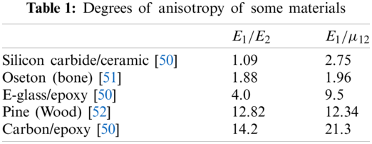
Anisotropic materials show various degrees of anisotropy. The largeness of the ratios E1/ E2 and E1/μ12 represents the degree of anisotropy of a material [50]. Degrees of the anisotropy of some materials are given in Table 1. This table includes materials with extremely low and extremely high degrees of anisotropy. The first material in Table 1 has a low degree of anisotropy, while the last one, i.e., the unidirectional Carbon/epoxy composite material, has an extremely high degree of anisotropy.

To investigate the effect of the distance between main and pseudo boundaries, i.e., δ, on the results, the number of source points and the magnitude of δ should be considered simultaneously. For a fixed value of δ, by a larger number of source pionts, there will be a rise in the condition number of the main matrix in the MFS. On the other hand, for a fixed number of source points, increasing the value of δ has the same effect and increases the condition number. Therefore, a parameter which describes the distance between main and pseudo boundaries relative to the number of soure points should be considered in the next numerical studies. Hematiyan et al. [34,40] defined the source point location parameter for this purpose. The source point location parameter can be defined using Fig. 1. The boundary points nearest to the source points Si and Si+1 are considered as the base points of these source points and are denoted by Bi and Bi+1, respectively. The base points do not necessarily coincide with collocation points. The location parameter of the source point Si is represented by K and is defined as follows:

K=δδ′, (23)

where δ and δ′ are the distance from Si to Bi and Bi+1, respectively (Fig. 1). For a fixed number of source points, narrowing the distance between the pseudo and main boundaries reduces the value of the location parameter and for a fixed distance between the pseudo and main boundaries, increasing the number of source points enlarges the value of the location parameter.

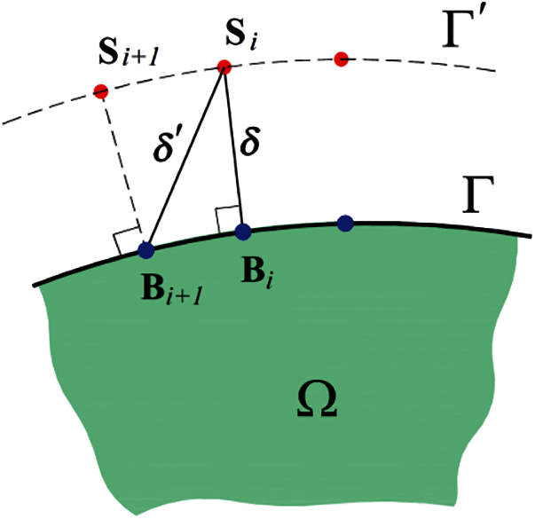
Figure 1: Configuration of source points on the pseudo boundary

Two types of anisotropic elastostatic problems can be analyzed by the MFS. In the first type, the boundary condition is of Dirichlet type and is prescribed by a function which satisfies the governing equation of the problem. In the second type, which is more practical, the boundary conditions are of mixed type and are prescribed by functions which do not satisfy the governing equations. As mentioned in reference [44], most examples studied in the previous works are of the first type. In this work, we take into account both types of problems; however, the main focus is maintained on the second type, which is more important.

4.1 A Circular Domain

A circular domain (disk) of unit radius centered at the origin of the coordinate system under the plane stress conditions is considered. The geometry of the disk is suitable for the MFS because it is simple and smooth. Simple boundary conditions of Dirichlet type are also considered for the problem. It is assumed that the radial and circumferential displacements of the boundary are ur = 1.0 and uθ=0, respectively. The boundary conditions of the problem in the Cartesian coordinate system can be expressed as follows:

u=x,v=y. (24)

The disk is assumed to be made of the unidirectional S-glass/epoxy composite material. The material is orthotropic and its elastic constants in its principal material directions are E1=45 GPa, E2=11 GPa, μ12=4.5 GPa, and ν12=0.29 [50]. It is assumed that the material direction makes an angle of π/6 with the x-direction. The exact displacement solution of the problem is the same as Eq. (24). The exact strain solution can be found using Eq. (3), which yields uniform strains and stresses in the domain.

We use the standard MFS with M = N = 16 to solve this problem. The collocation points are uniformly distributed on the circle. We examine four cases with different values for the source point location parameter (K). The values selected for K are 0.9, 0.95, 0.97, and 0.99. The corresponding values of δ in these four cases are 1.193, 2.085, 3.185, and 8.392, respectively. The results for radial displacement and Cartesian components of stress in comparison with exact solutions are shown in Figs. 2–5. The exact solution for radial displacement and stresses are uniform over the boundary of the disk; however, the solutions obtained by the MFS have some oscillations over the boundary in the cases with smaller values of K.

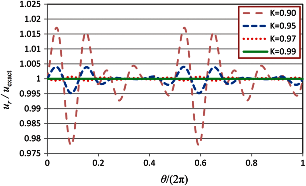
Figure 2: Radial displacement over the boundary of the disk

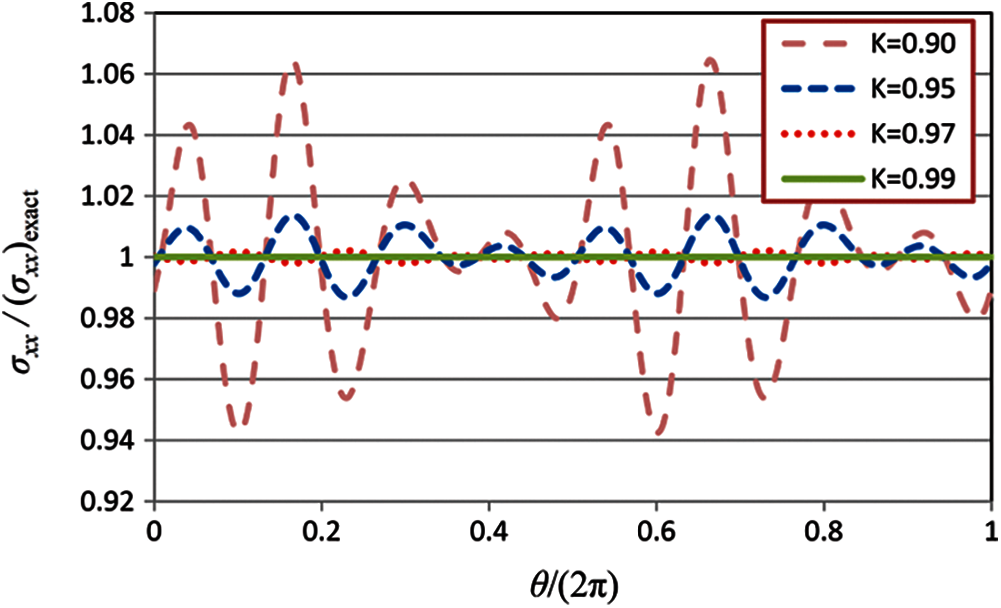
Figure 3: Normal stress in the x-direction over the boundary of the disk

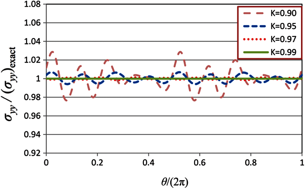
Figure 4: Normal stress in the y-direction over the boundary of the disk

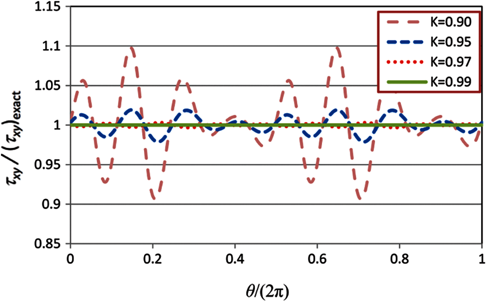
Figure 5: Shearing stress over the boundary of the disk

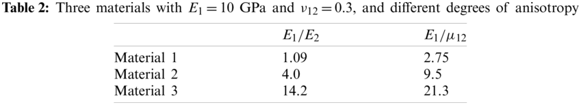
It is observed that by increasing the value of K, the accuracy of the solutions is enhanced. The MFS results for isotropic elastostatic problems [40] show that K = 0.85 yields sufficiently accurate results; however, as it is seen in Fig. 5, the MFS results with K = 0.9 for the present example, which has a moderate degree of anisotropy, are not sufficiently accurate. For better clarification, we solve the problem with three materials with different degrees of anisotropy. The elastic properties of the three materials are given in Table 2. E1 and ν12 are the same for the three materials. Material 1 has a low degree of anisotropy (same as the first material in Table 1) and Material 3 has a high degree of anisotropy (same as the last material in Table 1). Similar to the previous case, it is assumed that the material direction makes an angle of π/6 with the x-direction.

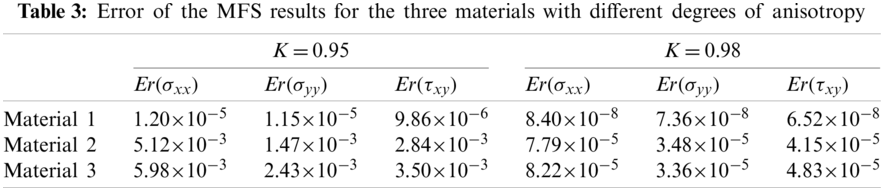
For each material, the problem is solved using the standard MFS (M = N = 16) with K = 0.95 and K = 0.98. The stress components at 160 test points on the boundary are obtained by the MFS and the relative error of each stress component is computed using the following equation:

Er(σij)=1160∑k=1160[(σijMFS)k−(σijExact)kσRef]2, (25)

where (σijMFS)k and (σijExact)k represent stress components at the kth test point obtained by the MFS and the exact solution, respectively, and σRef=max(σxx,σyy,τxy). The errors of the MFS results are reported in Table 3. As can be seen, the error significantly increases as the degree of anisotropy is higher. It is also observed that as the value of the location parameter increases, the error of the obtained solution is reduced.

4.2 A Rectangular Plate with a Hole

In the previous section, a disk with a simple boundary condition was considered. In this section, a complicated geometry with more challenging boundary conditions is considered. As shown in Fig. 6, a rectangular plate with a fixed hole is considered. The upper and right edges of the rectangle are subjected to uniform compressive and tensile tractions, respectively. The material principal directions make an angle of π/4 (45∘) with the global coordinates system. The outer boundary is not smooth and high stress concentrations occur at two points on the circle. The three materials listed in Table 2 are used and the problem is solved many times with different numbers of source points and collocation points. Moreover, different values for the location parameter of source points are examined. In each case, the collocation points are uniformly distributed on the boundaries and the geometry of the pseudo boundaries is assumed similar to the main boundaries.

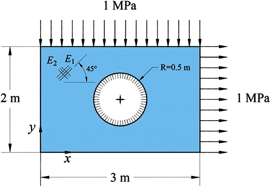
Figure 6: Rectangular plate with a fixed hole

There is no exact solution for this problem. An accurate reference solution is obtained by the finite element method (FEM) with a fine mesh using ANSYS software. Maximum absolute values of stresses occur on the circle and the error of solution is defined in terms of these stresses as follows:

Er=13[((σxx)maxMFS−(σxx)maxFEM(σxx)maxFEM)2+((σyy)maxMFS−(σyy)maxFEM(σyy)maxFEM)2+((τxy)maxMFS−(τxy)maxFEM(τxy)maxFEM)2]1/2. (26)

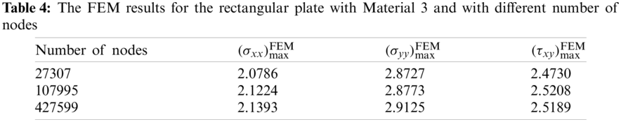
Importantly, a large number of nodes and elements should be considered for finite element (FE) analysis of this problem to obtain relatively accurate solutions. In Table 4, the FEM results for critical stresses are listed. The results in Table 4 are associated with Material 3. As it is observed, a large number of nodes are required to achieve solutions accurate to two decimal places.

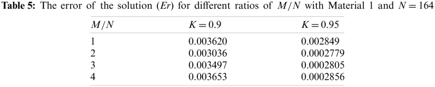
In the first case, the problem with Material 1 is solved using the MFS. Since the degree of the anisotropy of Material 1 is relatively small, by considering only 164 source points (100 and 64 source points for outer and inner boundaries, respectively), sufficiently accurate solutions can be obtained. Moreover, we consider different values of the location parameter of source points, i.e., K, and different ratios of the number of collocation points to the number of source points, i.e., M / N. The errors of the results for this case with Material 1 are reported in Table 5. As observed, the solutions with K = 0.95 is slightly more accurate than K = 0.9. Moreover, the results with M /N > 1 are better than the standard MFS with M /N = 1. However, it is observed that increasing the ratio M /N greater than 2 has no significant effect on the accuracy of the results. Therefore, the value of 2 can be a good suggestion for the ratio M / N.

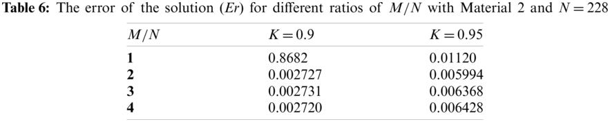
In the second case, the problem with Material 2, which has a higher degree of anisotropy, is solved. In this case, 100+128 = 228 source points, i.e., 100 source points for the outer boundary and 128 source points for the inner boundary, are considered instead of 164. The corresponding errors are listed in Table 6. As seen in this table, the solution obtained by considering M / N = 2 is far more accurate than M / N = 1. Similarly, increasing the ratio M / N more than 2 has no significant effect on the accuracy of the solution. Remarkably, by increasing the value of K, i.e., increasing the distance between main and pseudo boundaries, the accuracy of the results is not enhanced in this case.

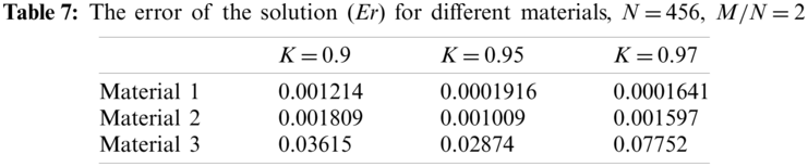
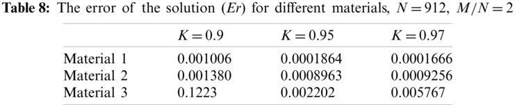
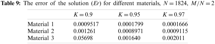
Solving the problem with Material 3 is far more difficult because the degree of anisotropy of Material 3 is larger than the previous cases. In Tables 7–9, the results for the cases with 200+256 = 456, 400+512 = 912, and 800+1024 = 1824 source points, for the problem with the three materials are given. M /N = 2 is considered in all cases. Evidently, the accuracy of the results for the case with Material 3 is considerably lower than the two materials with smaller degrees of anisotropy. Moreover, increasing the distance between main and pseudo boundaries does not necessarily enhance the accuracy of the results, which is in contrast with the previous problem (disk) where by increasing the distance between the main and pseudo boundaries, the error of the results was reduced.

For better clarification, the contours of the stress components in the rectangular plate obtained by the FEM with 427599 nodes, and by the MFS with 912 source points and M/ N = 2 are shown in Figs. 7–9. The variations of stress components on the internal circle are also shown in Figs. 10–12. These figures demonstrate that the stress solutions obtained by the MFS are in very good agreement with those obtained by the FEM. Moreover, the complicated distribution of stresses in the domain and the stress concentrations at some locations on the circle are clearly shown in these figures.

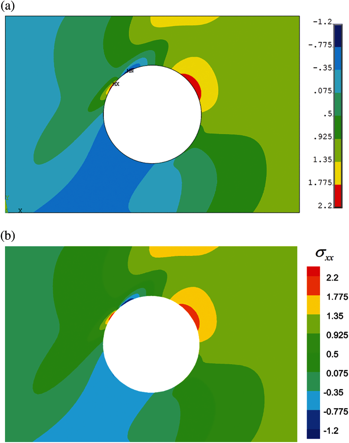
Figure 7: Contours of normal stress in the x-direction (in MPa) in the case with Material 3, (a) FEM with 427599 nodes, (b) MFS with N = 912 and M /N = 2

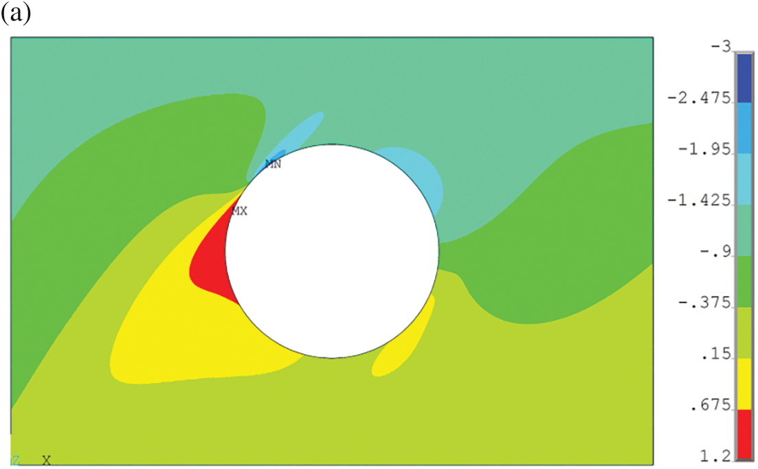
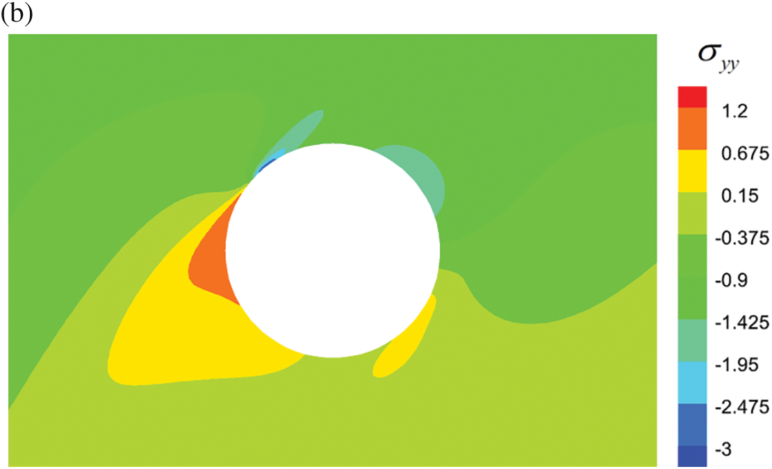
Figure 8: Contours of normal stress in the y-direction (in MPa) in the case with Material 3, (a) FEM with 427599 nodes, (b) MFS with N = 912 and M /N = 2

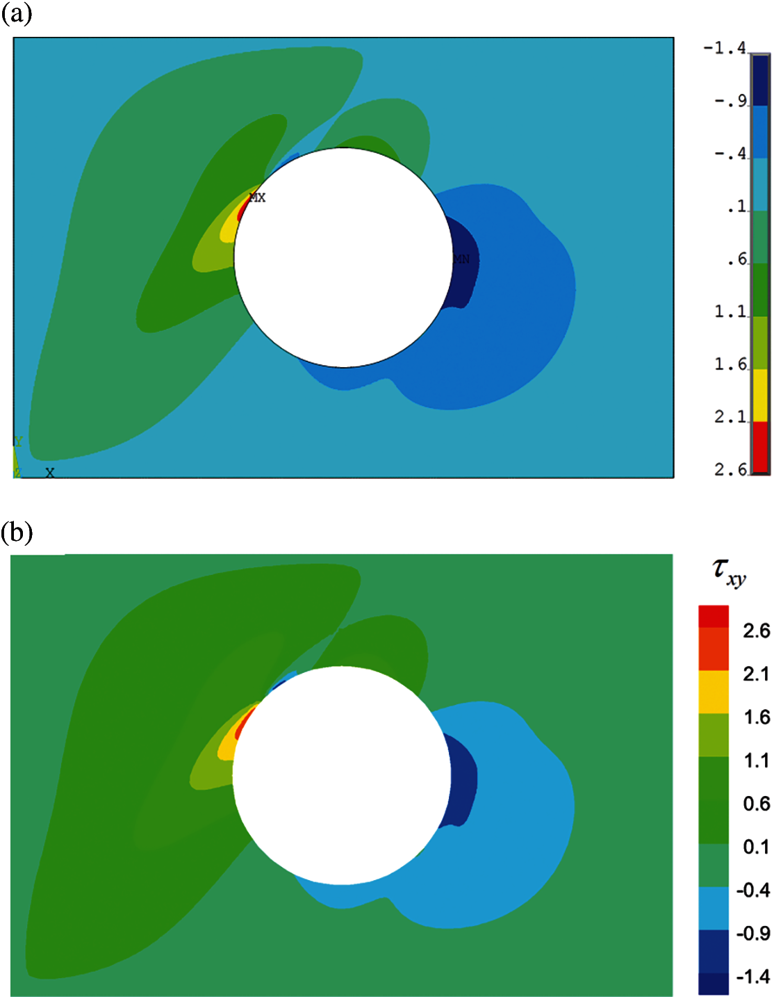
Figure 9: Contours of shearing stress (in MPa) in the case with Material 3, (a) FEM with 427599 nodes, (b) MFS with N = 912 and M /N = 2

Figure 10: Normal stress in the x-direction on the internal circle obtained by the FEM with 427599 nodes and by the MFS with N = 912, M/N = 2, and Material 3

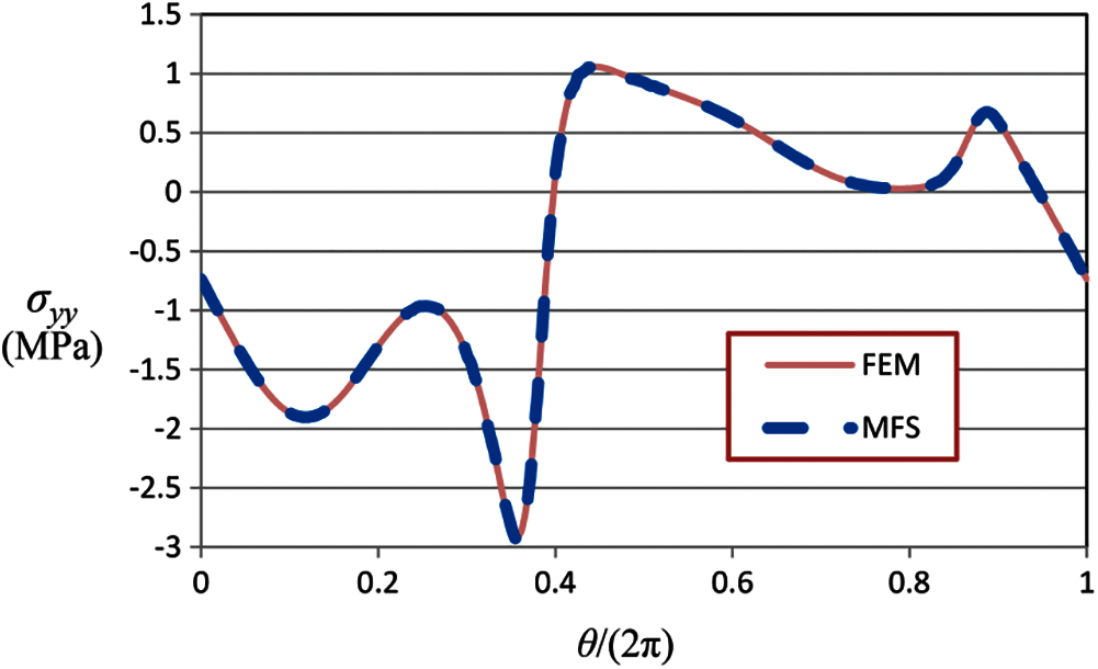
Figure 11: Normal stress in the y-direction on the internal circle obtained by the FEM with 427599 nodes and by the MFS with N = 912, M /N = 2, and Material 3

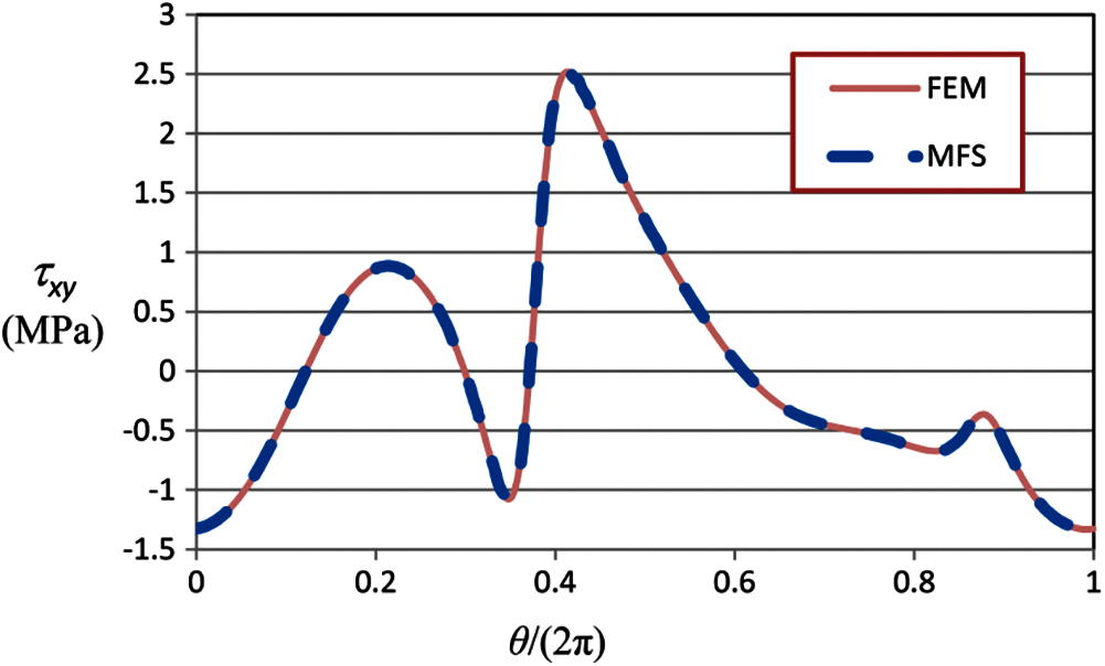
Figure 12: Shearing stress on the internal circle obtained by the FEM with 427599 nodes and by the MFS with N = 912, M/N = 2, and Material 3

5  Conclusions

The important parameters, which have significant influence on the accuracy of the MFS for the analysis of two-dimensional anisotropic elastostatic problems, were numerically studied in this work. Although the findings reported in this research is not based on mathematical analysis, some suggestions regarding the MFS for the elastostatic analysis of anisotropic bodies are offered that can help solve practical problems. According to the numerical studies conducted in the work, the following conclusions are drawn:

•   Three materials with low, moderate, and high degrees of anisotropy were examined in simple and complicated elastostatic problems. As observed, in the same conditions, the accuracy of the results corresponding to the problem with highly anisotropic material was far lower than the same problem with lower degree of anisotropy.

•   Anisotropic elastostatic problems with simple geometry and simple boundary conditions can be efficiently solved using the standard MFS with equal numbers of source and collocation points, i.e., M/N = 1.

•   For anisotropic elastostatic problems with complicated geometry and/or complicated boundary conditions, more collocation points than source points render far more accurate results. Through the examples presented in this work, it was observed that M /N = 2 could be a suitable choice.

•   In simple problems, raising the value of K, i.e., increasing the distance between main and pseudo boundaries, enhances the accuracy of the results; however, it is not the case for complicated problems. It should also be mentioned that in the cases where the value of K is small, i.e., the distance between main and pseudo boundaries is small relative to the distance between source points, some undesired oscillations of variables occur on the boundary. In other words, in complicated anisotropic elastostatic problems, it may be necessary to find a suitable distance between main and pseudo boundaries by a trial and error procedure or by an optimization process. As the starting value, K = 0.95 is suggested for the location parameter of source points in these cases.

Unlike the element-based methods, meshfree methods do not require any re-meshing process [53]. This advantage makes the proposed boundary-type meshfree method particularly suitable for some practical problems. In the follow-up works, shape optimization problems and inverse problems for the identification of elastic constants [54] or reconstruction of boundary conditions of anisotropic bodies can be considered. Recently, domain-type meshfree methods have been employed for the analysis of contact problems [55–57]. The proposed method may also be used for analysis of contact problems. Future research may focus on analyzing the mechanical behavior of polycrystalline structures [58,59] using the MFS.

Funding Statement: The first author would like to acknowledge the support received from the Vice Chancellor of Research at Shiraz University under Grant No. 99GRC1M1820.

Conflicts of Interest: The authors declare that they have no conflicts of interest to report regarding the present study.

References

 1.  Tsai, C. C., Lin, Y. C., Young, D. L., Atluri, S. N. (2006). Investigations on the accuracy and condition number for the method of fundamental solutions. Computer Modeling in Engineering & Sciences, 16(2), 103. DOI 10.3970/cmes.2006.016.103. [Google Scholar] [CrossRef]

 2.  Alves, C. J. (2009). On the choice of source points in the method of fundamental solutions. Engineering Analysis with Boundary Elements, 33(12), 1348–1361. DOI 10.1016/j.enganabound.2009.05.007. [Google Scholar] [CrossRef]

 3.  Tsai, C. C., Young, D. L. (2013). Using the method of fundamental solutions for obtaining exponentially convergent helmholtz eigensolutions. Computer Modeling in Engineering & Sciences, 94(2), 175–205. DOI 10.3970/cmes.2013.094.175. [Google Scholar] [CrossRef]

 4.  Liu, G. R., Gu, Y. T. (2005). An introduction to meshfree methods and their programming. Dordrecht, The Netherland: Springer Science & Business Media. [Google Scholar]

 5.  Wang, L., Chen, J. S., Hu, H. Y. (2010). Subdomain radial basis collocation method for fracture mechanics. International Journal for Numerical Methods in Engineering, 83(7), 851–876. DOI 10.1002/nme.2860. [Google Scholar] [CrossRef]

 6.  Wang, L., Qian, Z. (2020). A meshfree stabilized collocation method (SCM) based on reproducing kernel approximation. Computer Methods in Applied Mechanics and Engineering, 371, 113303. DOI 10.1016/j.cma.2020.113303. [Google Scholar] [CrossRef]

 7.  Wang, L., Liu, Y., Zhou, Y., Yang, F. (2021). Static and dynamic analysis of thin functionally graded shell with in-plane material inhomogeneity. International Journal of Mechanical Sciences, 193, 106165. DOI 10.1016/j.ijmecsci.2020.106165. [Google Scholar] [CrossRef]

 8.  Zhang, J., Zhou, G., Gong, S., Wang, S. (2017). Transient heat transfer analysis of anisotropic material by using element-free galerkin method. International Communications in Heat and Mass Transfer, 84, 134–143. DOI 10.1016/j.icheatmasstransfer.2017.04.003. [Google Scholar] [CrossRef]

 9.  Dadar, N., Hematiyan, M. R., Khosravifard, A., Shiah, Y. C. (2020). An inverse meshfree thermoelastic analysis for identification of temperature-dependent thermal and mechanical material properties. Journal of Thermal Stresses, 43(9), 1165–1188. DOI 10.1080/01495739.2020.1775534. [Google Scholar] [CrossRef]

10. Chen, J. S., Yoon, S., Wu, C. T. (2002). Non-linear version of stabilized conforming nodal integration for galerkin mesh-free methods. International Journal for Numerical Methods in Engineering, 53(12), 2587–2615. DOI 10.1002/(ISSN)1097-0207. [Google Scholar] [CrossRef]

11. Hematiyan, M. R., Khosravifard, A., Liu, G. R. (2014). A background decomposition method for domain integration in weak-form meshfree methods. Computers & Structures, 142, 64–78. DOI 10.1016/j.compstruc.2014.07.001. [Google Scholar] [CrossRef]

12. Jamshidi, B., Hematiyan, M. R., Mahzoon, M. (2019). An improved time domain meshfree method for analysis of quasi-static and dynamic inhomogeneous viscoelastic problems. Engineering Analysis with Boundary Elements, 106, 59–67. DOI 10.1016/j.enganabound.2019.04.031. [Google Scholar] [CrossRef]

13. Marin, L. (2010). Regularized method of fundamental solutions for boundary identification in two-dimensional isotropic linear elasticity. International Journal of Solids and Structures, 47(24), 3326–3340. DOI 10.1016/j.ijsolstr.2010.08.010. [Google Scholar] [CrossRef]

14. Bin-Mohsin, B., Lesnic, D. (2012). Determination of inner boundaries in modified helmholtz inverse geometric problems using the method of fundamental solutions. Mathematics and Computers in Simulation, 82(8), 1445–1458. DOI 10.1016/j.matcom.2012.02.002. [Google Scholar] [CrossRef]

15. Johansson, B. T., Lesnic, D., Reeve, T. (2013). A meshless regularization method for a two-dimensional two-phase linear inverse stefan problem. Advances in Applied Mathematics and Mechanics, 5(6), 825–845. DOI 10.4208/aamm.2013.m77. [Google Scholar] [CrossRef]

16. Mohammadi, M., Hematiyan, M. R., Shiah, Y. C. (2018). An efficient analysis of steady-state heat conduction involving curved line/surface heat sources in two/three-dimensional isotropic media. Journal of Theoretical and Applied Mechanics, 56, 1123–1137. DOI 10.15632/jtam-pl.56.4.1123. [Google Scholar] [CrossRef]

17. Mohammadi, M., Hematiyan, M. R., Khosravifard, A. (2019). Analysis of two-and three-dimensional steady-state thermo-mechanical problems including curved line/surface heat sources using the method of fundamental solutions. European Journal of Computational Mechanics, 28, 51–80. DOI 10.13052/ejcm1958-5829.28123. [Google Scholar] [CrossRef]

18. Mohammadi, M. (2019). The method of fundamental solutions for two-and three-dimensional transient heat conduction problems involving point and curved line heat sources. Iranian Journal of Science and Technology, Transactions of Mechanical Engineering, 45, 993–1005. DOI 10.1007/s40997-019-00333-9. [Google Scholar] [CrossRef]

19. Mohammadi, M., Hematiyan, M. R. (2021). Analysis of transient uncoupled thermoelastic problems involving moving point heat sources using the method of fundamental solutions. Engineering Analysis with Boundary Elements, 123, 122–132. DOI 10.1016/j.enganabound.2020.11.015. [Google Scholar] [CrossRef]

20. Gao, X. W. (2010). An effective method for numerical evaluation of general 2D and 3D high order singular boundary integrals. Computer Methods in Applied Mechanics and Engineering, 199(45–48), 2856–2864. DOI 10.1016/j.cma.2010.05.008. [Google Scholar] [CrossRef]

21. Hematiyan, M. R., Khosravifard, A., Bui, T. Q. (2013). Efficient evaluation of weakly/strongly singular domain integrals in the BEM using a singular nodal integration method. Engineering Analysis with Boundary Elements, 37(4), 691–698. DOI 10.1016/j.enganabound.2013.02.004. [Google Scholar] [CrossRef]

22. Shiah, Y. C., Hematiyan, M. R., Chen, Y. H. (2013). Regularization of the boundary integrals in the BEM analysis of 3D potential problems. Journal of Mechanics, 29(3), 385–401. DOI 10.1017/jmech.2012.140. [Google Scholar] [CrossRef]

23. Zhang, Y., Li, X., Sladek, V., Sladek, J., Gao, X. (2014). Computation of nearly singular integrals in 3D BEM. Engineering Analysis with Boundary Elements, 48, 32–42. DOI 10.1016/j.enganabound.2014.07.004. [Google Scholar] [CrossRef]

24. Raamachandran, J., Rajamohan, C. (1996). Analysis of composite plates using charge simulation method. Engineering Analysis with Boundary Elements, 18(2), 131–135. DOI 10.1016/S0955-7997(96)00042-2. [Google Scholar] [CrossRef]

25. Berger, J. R., Karageorghis, A. (2001). The method of fundamental solutions for layered elastic materials. Engineering Analysis with Boundary Elements, 25(10), 877–886. DOI 10.1016/S0955-7997(01)00002-9. [Google Scholar] [CrossRef]

26. Tsai, C. C. (2007). The method of fundamental solutions for three-dimensional elastostatic problems of transversely isotropic solids. Engineering Analysis with Boundary Elements, 31(7), 586–594. DOI 10.1016/j.enganabound.2006.12.004. [Google Scholar] [CrossRef]

27. Hematiyan, M. R., Mohammadi, M., Tsai, C. C. (2021). The method of fundamental solutions for anisotropic thermoelastic problems. Applied Mathematical Modelling, 95, 200–218. DOI 10.1016/j.apm.2021.02.001. [Google Scholar] [CrossRef]

28. Liu, Q. G., Šarler, B. (2014). Non-singular method of fundamental solutions for anisotropic elasticity. Engineering Analysis with Boundary Elements, 45, 68–78. DOI 10.1016/j.enganabound.2014.01.020. [Google Scholar] [CrossRef]

29. Liu, Q. G., Fan, C. M., Šarler, B. (2021). Localized method of fundamental solutions for two-dimensional anisotropic elasticity problems. Engineering Analysis with Boundary Elements, 125, 59–65. DOI 10.1016/j.enganabound.2021.01.008. [Google Scholar] [CrossRef]

30. Gu, Y., Fan, C. M., Fu, Z. (2021). Localized method of fundamental solutions for three-dimensional dlasticity problems: Theory. Advances in Applied Mathematics and Mechanics, 13(6), 1520–1534. DOI 10.4208/aamm. [Google Scholar] [CrossRef]

31. Wong, K. Y., Ling, L. (2011). Optimality of the method of fundamental solutions. Engineering Analysis with Boundary Elements, 35(1), 42–46. DOI 10.1016/j.enganabound.2010.06.002. [Google Scholar] [CrossRef]

32. Liu, C. S. (2012). An equilibrated method of fundamental solutions to choose the best source points for the laplace equation. Engineering Analysis with Boundary Elements, 36(8), 1235–1245. DOI 10.1016/j.enganabound.2012.03.001. [Google Scholar] [CrossRef]

33. Li, M., Chen, C. S., Karageorghis, A. (2013). The MFS for the solution of harmonic boundary value problems with non-harmonic boundary conditions. Computers & Mathematics with Applications, 66(11), 2400–2424. DOI 10.1016/j.camwa.2013.09.004. [Google Scholar] [CrossRef]

34. Hematiyan, M. R., Haghighi, A., Khosravifard, A. (2017). A two-constraint method for appropriate determination of the configuration of source and collocation points in the method of fundamental solutions for 2D laplace equation. Advances in Applied Mathematics and Mechanics, 10(3), 554–580. DOI 10.4208/aamm.OA-2016-0065. [Google Scholar] [CrossRef]

35. Grabski, J. K., Karageorghis, A. (2019). Moving pseudo-boundary method of fundamental solutions for nonlinear potential problems. Engineering Analysis with Boundary Elements, 105, 78–86. DOI 10.1016/j.enganabound.2019.04.009. [Google Scholar] [CrossRef]

36. Karageorghis, A. (2009). A practical algorithm for determining the optimal pseudo-boundary in the method of fundamental solutions. Advances in Applied Mathematics and Mechanics, 1(4), 510–528. DOI 10.4208/aamm.09-m0916. [Google Scholar] [CrossRef]

37. Chen, C. S., Karageorghis, A., Li, Y. (2016). On choosing the location of the sources in the MFS. Numerical Algorithms, 72(1), 107–130. DOI 10.1007/s11075-015-0036-0. [Google Scholar] [CrossRef]

38. Gorzelańczyk, P., Kołodziej, J. A. (2008). Some remarks concerning the shape of the source contour with application of the method of fundamental solutions to elastic torsion of prismatic rods. Engineering Analysis with Boundary Elements, 32(1), 64–75. DOI 10.1016/j.enganabound.2007.05.004. [Google Scholar] [CrossRef]

39. Grabski, J. K. (2019). On the sources placement in the method of fundamental solutions for time-dependent heat conduction problems. Computers & Mathematics with Applications, 88, 33–51. DOI 10.1016/j.camwa.2019.04.023. [Google Scholar] [CrossRef]

40. Hematiyan, M. R., Arezou, M., Dezfouli, N. K., Khoshroo, M. (2019). Some remarks on the method of fundamental solutions for two-dimensional elasticity. Computer Modelling in Engineering & Sciences, 121(2), 661–686. DOI 10.32604/cmes.2019.08275. [Google Scholar] [CrossRef]

41. Dezfouli, N. K., Hematiyan, M. R., Mohammadi, M. (2021). A modification of the method of fundamental solutions for solving 2D problems with concave and complicated domains. Engineering Analysis with Boundary Elements, 123, 168–181. DOI 10.1016/j.enganabound.2020.11.016. [Google Scholar] [CrossRef]

42. Khoshroo, M., Hematiyan, M. R., Daneshbod, Y. (2020). Two-dimensional elastodynamic and free vibration analysis by the method of fundamental solutions. Engineering Analysis with Boundary Elements, 117, 188–201. DOI 10.1016/j.enganabound.2020.04.014. [Google Scholar] [CrossRef]

43. Sadd, M. H. (2009). Elasticity: Theory, applications, and numeric. Fourth edition. Oxford, UK: Academic Press. [Google Scholar]

44. Cheng, A. H., Hong, Y. (2020). An overview of the method of fundamental solutions–-Solvability, uniqueness, convergence, and stability. Engineering Analysis with Boundary Elements, 120, 118–152. DOI 10.1016/j.enganabound.2020.08.013. [Google Scholar] [CrossRef]

45. Lekhnitski, S. G. (1963). Theory of elasticity of an anisotropic elastic body. San Francisco: Holden-day Series in Mathematical Physics. [Google Scholar]

46. Cruse, T. A. (1988). Boundary element analysis in computational fracture mechanics. Dordrecht, Netherlands: Kluwer Academic Publishers. [Google Scholar]

47. Aliabadi, M. H. (2002). The boundary element method: Applications in solids and structures, vol. 2. Chichester, England: John Wiley & Sons. [Google Scholar]

48. Sollero, P., Aliabadi, M. H. (1993). Fracture mechanics analysis of anisotropic plates by the boundary element method. International Journal of Fracture, 64(4), 269–284. DOI 10.1007/BF00017845. [Google Scholar] [CrossRef]

49. Hematiyan, M. R., Khosravifard, A., Shiah, Y. C., Tan, C. L. (2012). Identification of material parameters of two-dimensional anisotropic bodies using an inverse multi-loading boundary element technique. Computer Modeling in Engineering & Sciences, 87(1), 55. DOI 10.3970/cmes.2012.087.055. [Google Scholar] [CrossRef]

50. Daniel, I. M., Ishai, O., Daniel, I. M., Daniel, I. (2006). Engineering mechanics of composite materials, vol. 1994. New York: Oxford University Press. [Google Scholar]

51. Franzoso, G. (2008). Elastic anisotropy of lamellar bone measured by nanoindentation (Ph.D. Thesis). Politecnico Di Milano, Milan, Italy. [Google Scholar]

52. Grekin, M., Surini, T. (2008). Shear strength and perpendicular-to-grain tensile strength of defect-free Scots pine wood from mature stands in Finland and Sweden. Wood Science and Technology, 42(1), 75–91. DOI 10.1007/s00226-007-0151-8. [Google Scholar] [CrossRef]

53. Xia, H., Gu, Y. (2021). Generalized finite difference method for electroelastic analysis of three-dimensional piezoelectric structures. Applied Mathematics Letters, 117, 107084. DOI 10.1016/j.aml.2021.107084. [Google Scholar] [CrossRef]

54. Hematiyan, M. R., Khosravifard, A., Shiah, Y. C. (2017). A new stable inverse method for identification of the elastic constants of a three-dimensional generally anisotropic solid. International Journal of Solids and Structures, 106, 240–250. DOI 10.1016/j.ijsolstr.2016.11.009. [Google Scholar] [CrossRef]

55. Huang, J., Nguyen-Thanh, N., Zhou, K. (2018). An isogeometric-meshfree coupling approach for contact problems by using the third medium method. International Journal of Mechanical Sciences, 148, 327–336. DOI 10.1016/j.ijmecsci.2018.08.031. [Google Scholar] [CrossRef]

56. Nguyen-Thanh, N., Li, W., Huang, J., Srikanth, N., Zhou, K. (2019). An adaptive isogeometric analysis meshfree collocation method for elasticity and frictional contact problems. International Journal for Numerical Methods in Engineering, 120(2), 209–230. DOI 10.1002/nme.6132. [Google Scholar] [CrossRef]

57. Li, W., Nguyen-Thanh, N., Zhou, K. (2020). An isogeometric-meshfree collocation approach for two-dimensional elastic fracture problems with contact loading. Engineering Fracture Mechanics, 223, 106779. DOI 10.1016/j.engfracmech.2019.106779. [Google Scholar] [CrossRef]

58. Nguyen-Thanh, N., Li, W., Huang, J., Zhou, K. (2020). Adaptive higher-order phase-field modeling of anisotropic brittle fracture in 3D polycrystalline materials. Computer Methods in Applied Mechanics and Engineering, 372, 113434. DOI 10.1016/j.cma.2020.113434. [Google Scholar] [CrossRef]

59. Li, W., Nguyen-Thanh, N., Zhou, K. (2020). Phase-field modeling of brittle fracture in a 3D polycrystalline material via an adaptive isogeometric-meshfree approach. International Journal for Numerical Methods in Engineering, 121(22), 5042–5065. DOI 10.1002/nme.6509. [Google Scholar] [CrossRef]

Appendix A: Transformation of Elastic Compliance Coefficients

Assume that the first principal material direction makes an angle of θ with the x-direction as shown in Fig. A1. Denoting the elastic compliance coefficients in the material coordinates system and in the global Cartesian coordinates system by a¯ij and aij, respectively, the transformation of the constants can be expressed as follows:

[a11a12a16a21a22a26a61a62a66]=[T]T[a¯11a¯120a¯21a¯22000a¯66][T], (27)

where

[T]=[cos2θsin2θ2sin⁡θcos⁡θsin2θcos2θ−2sin⁡θcos⁡θ−sin⁡θcos⁡θsin⁡θcos⁡θcos2θ−sin2θ]. (28)

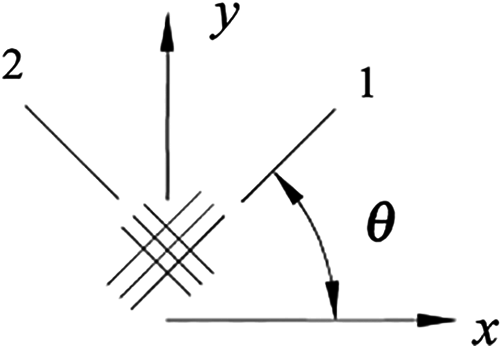
Figure 13: The angle between principal material directions and global Cartesian coordinates

This work is licensed under a Creative Commons Attribution 4.0 International License, which permits unrestricted use, distribution, and reproduction in any medium, provided the original work is properly cited.