| Computer Modeling in Engineering & Sciences |
DOI: 10.32604/cmes.2022.017799
ARTICLE
Pattern-Moving-Based Parameter Identification of Output Error Models with Multi-Threshold Quantized Observations
1School of Automation and Electrical Engineering, University of Science and Technology Beijing; Key Laboratory of Knowledge Automation for Industrial Processes, Ministry of Education, Beijing, 100083, China
2School of Information Engineering, Jingdezhen University, Jingdezhen, 333000, China
*Corresponding Author: Zhengguang Xu. Email: xzgustb@163.com
Received: 08 June 2021; Accepted: 03 September 2021
Abstract: This paper addresses a modified auxiliary model stochastic gradient recursive parameter identification algorithm (M-AM-SGRPIA) for a class of single input single output (SISO) linear output error models with multi-threshold quantized observations. It proves the convergence of the designed algorithm. A pattern-moving-based system dynamics description method with hybrid metrics is proposed for a kind of practical single input multiple output (SIMO) or SISO nonlinear systems, and a SISO linear output error model with multi-threshold quantized observations is adopted to approximate the unknown system. The system input design is accomplished using the measurement technology of random repeatability test, and the probabilistic characteristic of the explicit metric value is employed to estimate the implicit metric value of the pattern class variable. A modified auxiliary model stochastic gradient recursive algorithm (M-AM-SGRA) is designed to identify the model parameters, and the contraction mapping principle proves its convergence. Two numerical examples are given to demonstrate the feasibility and effectiveness of the achieved identification algorithm.
Keywords: Pattern moving; multi-threshold quantized observations; output error model; auxiliary model; parameter identification
In the metallurgical, petroleum-chemical and steel industries, there are technologically complicated, highly energy-consuming and polluting large-scale equipments such as electrolytic tank, sintering machine, blast furnace cement rotary kiln and so on. The production process of this kind of equipments presents the following characteristics [1]. 1) The complex system mechanism beyonds the accurate description of mathematical and physical equations; 2) Working conditions and quality parameters are in large quantities, and the system moving mode is full of distributiveness, nonlinearity and parameter perturbations; 3) Some physical and chemical processes are in conformity with statistical law of moving. A feasible method of system modeling and control is the pattern recognition technology for these considered processes [2] and most researchers’ practice is to design the corresponding model and controller according to the different pattern class of the system working condition [3,4]. A novel pattern-moving-based system dynamics description method was proposed in [5]. Its basic idea is to take the pattern class as a moving variable, and it is mapped to a computable space by class centers [6,7], interval numbers [8], and cells [9] due to its lack of arithmetic operation attribute. Furthermore, in view of various metric methods of pattern class, the linear autoregressive model with exogenous input (ARX) or interval ARX (IARX) model was established, and the parameter identification algorithm based on least square [6], minimum-variance-based controller [5], optimal controller [10], state-feedback controller [7] and predictive controller [11] were designed.
Although a series of research achievements have been made in the system modeling, parameter identification and control based on pattern moving, the differences of each pattern sample in one pattern class have never been considered. Since a pattern class is a set of pattern samples with the same or similar characteristics, the hybrid metrics, that is, the combination of implicit metric
The system with multi-threshold quantized observations is considered as a set-valued system which is different from a conventional one with accurate measurement outputs [19,20]. Although the identification of set-valued systems is not easy task, a series of important research results have been achieved in the past decade. For the linear system identification with threshold quantized observations, a full rank input design method (such as repetitive input design) and an empirical distribution function method were proposed in [21–23]. For the identification of Hammerstein and Wiener systems with binary outputs, the methods of proportional full rank signal, joint identifiability and strong full rank periodic signal inputs were proposed in [24,25], which effectively overcame the problems of system nonlinearity and rough binary output information. The parameter identification of Wiener system was also studied in terms of quantized inputs and binary outputs in [26]. Based on the truncated empirical measurement method of probabilistic statistics, a non-truncated empirical measurement method was proposed for the finite impulse response (FIR) system model with binary outputs, and the progressive effectiveness of the algorithm was demonstrated in [27]. A two-segment design method for a class of FIR systems with binary-valued observations was investigated in [28]. The parameter estimation problem of set-valued system was explained comprehensively from the perspective of combining system principle and practical application in [29]. The idea of parameter identification based on an auxiliary model was systematically expounded in [30]. An auxiliary-model-based least squares recursive algorithm was proposed for a quantized control system with communication constraints in [31].
This work investigates a M-AM-SGRPIA for a kind of linear output error models with multi-threshold quantized observations which is established from the perspective of pattern moving and hybrid metrics. Compared with the existed research results, the main differences and contributions of this paper are summarized as follows:
1) Different from the previous system identification problem of ARX or IARX models based on pattern moving and single metric [6,7], this paper considers hybrid metrics, the model noise distribution and proves the convergence of the designed M-AM-SGRPIA.
2) Compared with the parameter identification algorithms of set-valued system in [21–29], this paper adopts an auxiliary model and designs a M-AM-SGRPIA, which will reduce the estimation error radio to some extern.
3) An auxiliary-model-based least squares recursive algorithm has been designed for a class of linear systems with communication constraints in [31], which is different from the designed algorithm and physical background in this paper.
The outline of this work is organized as follows. Section 2 presents a pattern-moving-based system dynamics description and problem formulation. Section 3 proposes a M-AM-SGRPIA and its convergence is proved by the contraction mapping principle in Section 4. Section 5 demonstrates the feasibility and effectiveness of the M-AM-SGRPIA by two numerical examples. The conclusion comes in Section 6.
Notation:
2 Preliminary and Problem Formulation
2.1 Pattern-Moving-Based System Dynamics Description
Consider a class of unknown SIMO non-affine nonlinear discrete-time systems as follows:
where
Assumption 2.1 The input of system (1) is bounded, i.e., a constant
A pattern-moving-based system dynamics description [32] corresponding to system (1) is proposed in the following three steps:
1) Feature extraction
2) Classification
3) Establishing the pattern-moving-based system dynamics equations. The input sequence
where
If the contribution rate of the first principal component information obtained by feature extraction
Remark 2.1 In the process of establishing the pattern-moving-based dynamics Eqs. (2) and (3), the condition of parameter configuration of classification method is to ensure that a certain pattern class corresponds to a specific quality index of the product [36]. Furthermore, a physical SISO nonlinear discrete-time system can also be transformed into a pattern-moving-based SISO system, but it does not need the first step of feature extraction process.
Although there inevitably unmodeled dynamics problems, it is common to employ a linear model to approximate the situation that the system (2) is unknown. Choosing a reasonable classification method such as a modified quantized control classification [36], the following linear output error model with multi-threshold quantized observations can be constructed for system (2)–(3).
where
Assumption 2.2 The input and output orders of the model are known and equal, that is,
Assumption 2.3
Under the Assumption 2.2, the first expression of model (4) can be written as follows:
where
If the input sequence
Remark 2.2 The model orders and cumulative distribution function of
3 Design of Parameter Identification Algorithm
3.1 Estimation of Implicit Metric Value
For the convenience of calculation,
where
The measurement technology of random repeatability test is employed to design the input
Lemma 3.1 ([31]) For the model (4) and the output sequence
Lemma 3.2 ([31]) Under the full order input sequence
where
According to Lemma 3.1 and Lemma 3.2, the estimation error sequence
where
To accomplish the identification task, it is necessary to determine the probability estimate
1) If
2) If
The
Due to the unknown variables
where
By introducing a convergence index
Remark 3.1 A truncation method is adopted to get the value
For the designed M-AM-SGRA, the following Lemma is given and its convergence is to be proved.
Lemma 4.1 ([31]) For the given M-AM-SGRA (11)–(15), the following inequalities hold.
where
Theorem 4.1 For the model (9) and the corresponding M-AM-SGRA (11)–(15), under the conditions that
and it is assumed that the following inequality holds
thus, the estimation error vector
Proof.
It is concluded from (11) that
where
Taking the norm of both sides of (21), one has
Since
According to Lemma 4.1, the sum of the third term on the right side of (23) from
It can be also derived from the martingale convergence Theorem that
Letting
One can sequentially get
Further, using the Kronecker Lemma (Lemma d.5.3 in [38]) for inequalities (27), (28) to yield
and
It is known from the above proof process that the parameter estimation error is continuous and bounded. Using (21), one obtains
Replacing
Taking the square on both sides of (31) and adopting the inequality
Since
Taking the sum from
where
and
According to Lemma 4.1, the following two inequalities can be obtained.
Using the above two inequalities, one has
Therefore,
and
The proof of this Theorem is completed.
Example 1: Consider a SISO linear output error model with multi-threshold quantized observations which has been established based on pattern-moving and hybrid metrics as follows.
where
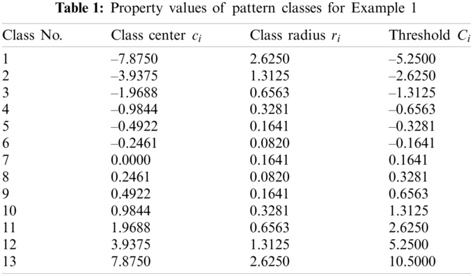
The size of input cycle is initially set as
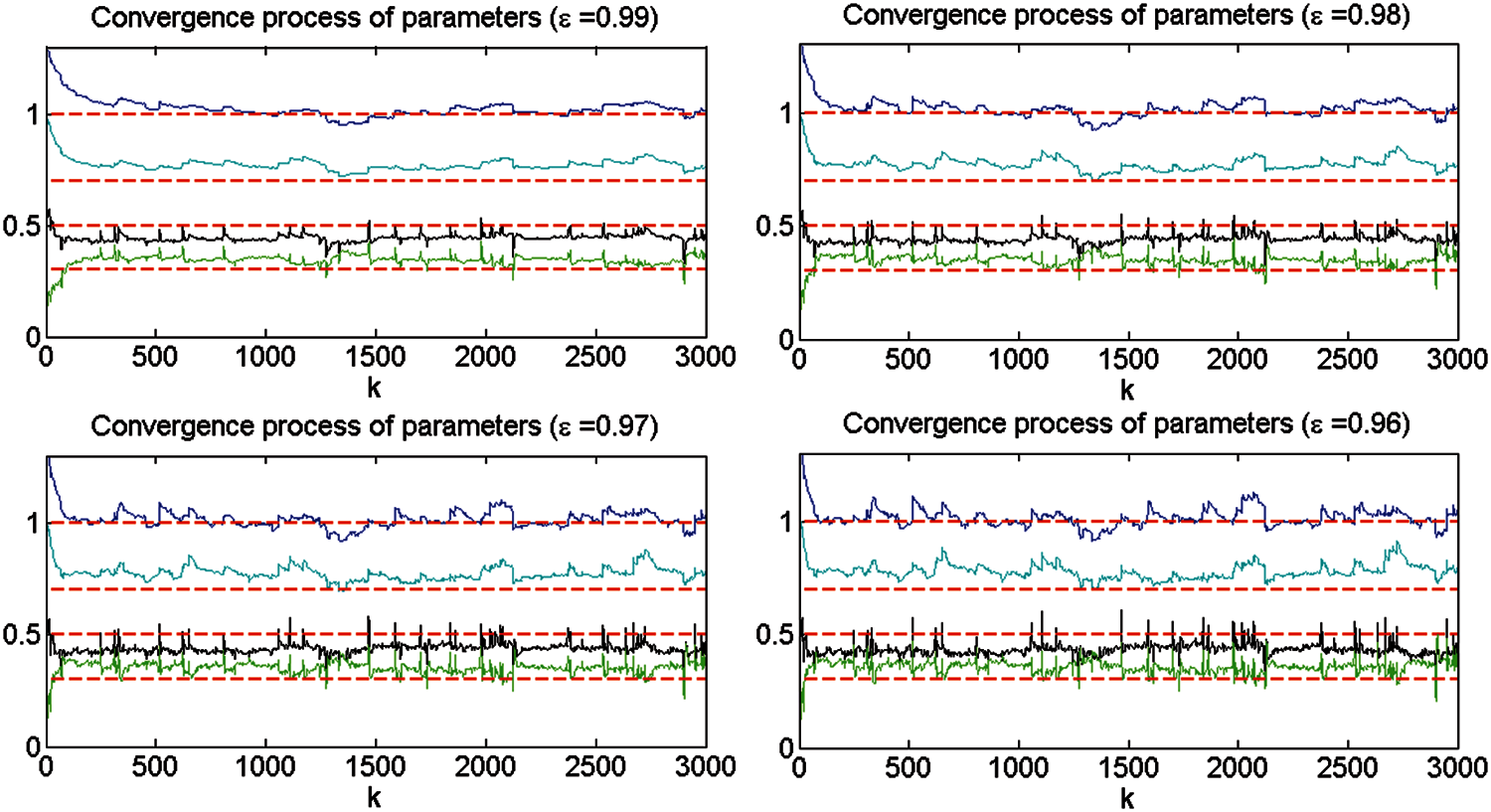
Figure 1: Convergence process of the M-AM-SGRA for Example 1
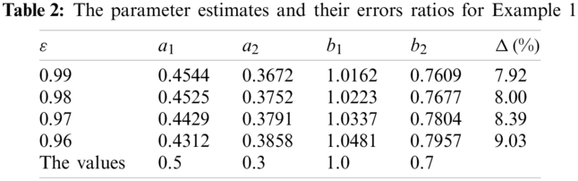
It is shown from Fig. 1 and Table 2 that the convergence index
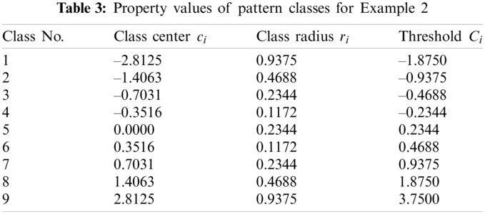
Example 2: Consider a SIMO unknown nonlinear system
where
1) Design of System input. The size of input cycle and the number of cycle are set the same as Example 1. The initial condition is set as
2) Classification and determining the actual output
where
Given the upper limit of the initial class radius
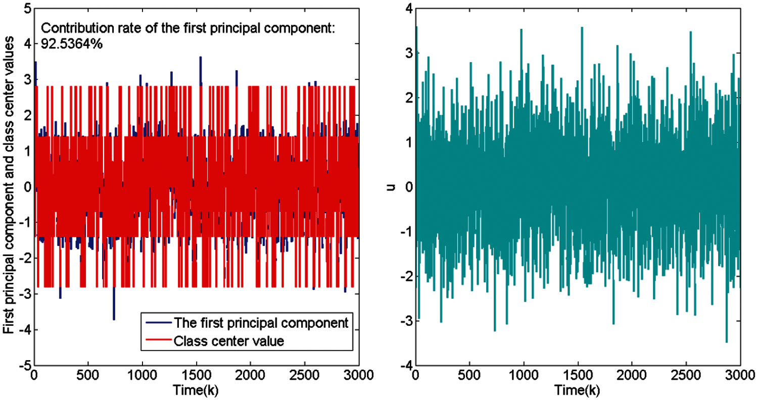
Figure 2: The distribution of
3) Establishing a pattern-moving-based linear output error model with multi-threshold quantized observations. According to the information obtained from the above steps, the pattern-moving-based system dynamics description Eqs. (2) and (3) is to be obtained. The input and output orders are assumed to be known
where
4) Model parameters identification. The designed M-AM-SGRA is employed to identify the model parameters. Referring to the conclusion of Example 1, the convergence factor
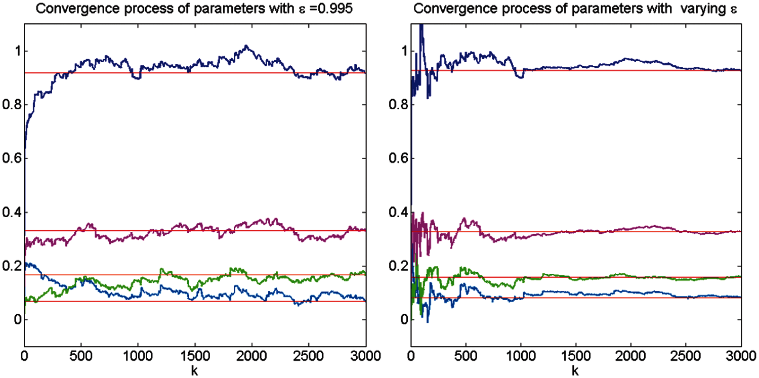
Figure 3: Convergence process of the M-AM-SGRA for Example 2
Remark 5.1 It is known to all that there exists many classifications and clustering methods in pattern recognition technology, such as C-means, ISODATA, and so on. Here a modified quantized control classification and class center explicit metric method is utilized. The initial parameters setting principle is based on the quality parameters of the product. In Example 2, it is assumed that the good quality is obtained with the output
According to the characteristics of classification and hybrid metrics, mappings are in line with the set-valued system, a linear output error model with multi-threshold quantized observations is adopted to approximate the unknown system, and an M-AM-SGRA is designed with its convergence proved. Finally, the validity and desired effect of the parameter identification algorithm is demonstrated by two numerical examples. Future works will focus on pattern-moving-based set-valued system modeling and control methods for achieving optimal robustness.
Funding Statement: This work was supported by the National Natural Science Foundation of China (62076025).
Conflicts of Interest: The authors declare that they have no conflicts of interest to report regarding the present study.
1. Qu, S. D. (1998). Pattern recognition approach to intelligent automation for complex industrial processes. Journal of University of Science and Technology Beijing, 20(4), 385–389. DOI 10.13374/j.issn1001-053x.1998.04.018. [Google Scholar] [CrossRef]
2. Saridis, G. N. (1981). Application of pattern recognition methods to control systems. IEEE Transactions on Automatic Control, 26(3), 638–645. DOI 10.1109/TAC.1981.1102685. [Google Scholar] [CrossRef]
3. Li, X., Zhang, L. (2011). Intelligent controller based on pattern recognition. ICECC, 1512–1515. DOI 10.1109/ICECC.2011.6066661. [Google Scholar] [CrossRef]
4. Yu, B., Zhang, X., Wu, L., Chen, X. (2020). A novel postprocessing method for robust myoelectric pattern-recognition control through movement pattern transition detection. IEEE Transactions on Human-Machine Systems, 50(1), 32–41. DOI 10.1109/THMS.2019.2953262. [Google Scholar] [CrossRef]
5. Xu, Z. G. (2001). Pattern recognition method of intelligent automation and its implementation in engineering (Ph.D. Thesis). University of Science and Technology Beijing [Google Scholar]
6. Wang, M. S., Xu, Z. G., Guo, L. L. (2017). Pattern recognition based dynamics description of production processes in metric spaces. Asian Journal of Control, 19(4), 1–13. DOI 10.1002/asjc.1471. [Google Scholar] [CrossRef]
7. Wang, M. S., Xu, Z. G., Guo, L. L. (2019). Stability and stabilization for a class of complex production processes via LMIs. Optimal Control Applications and Methods, 40(3), 460–478. DOI 10.1002/oca.2488. [Google Scholar] [CrossRef]
8. Sun, C. P., Xu, Z. G. (2016). Multi-dimensional moving pattern prediction based on multi-dimensional interval T-S fuzzy model. Control and Decision, 31(9), 1569–1576. DOI 10.13195/j.kzyjc.2015.0944. [Google Scholar] [CrossRef]
9. Guo, L. L., Xu, Z. G., Wang, Y. (2014). Dynamic modeling and optimal control for complex systems with statistical trajectory. Discrete Dynamics in Nature & Society, 2014(1), 1–8. DOI 10.1155/2015/245685. [Google Scholar] [CrossRef]
10. Xu, Z. G., Wu, J. X., Guo, L. L. (2013). Modeling and optimal control based on moving pattern. Chinese Control Conference, pp. 7894–7899. Xi'an, China. [Google Scholar]
11. Xu, Z. G., Wu, J. X. (2012). Data-driven pattern moving and generalized predictive control. IEEE International Conference on Systems, Man and Cybernetics, 1604–1609. DOI 10.1109/ICSMC.2012.6377966. [Google Scholar] [CrossRef]
12. Ljung, L. (1999). System identification: Theory for the user. 2nd ed. Englewood Cliffs: Prentice-Hall. [Google Scholar]
13. Clarke, D. W. (1967). Generalized least squares estimation of the parameters of a dynamic model. Proceeding of IFAC Symposium on Identification in Automatic Control Systems. Prague. [Google Scholar]
14. Astrom, K. J. (1980). Maximum likelihood and prediction error methods. Automatica, 16(5), 551–574. DOI 10.1016/0005-1098(80)90078-3. [Google Scholar] [CrossRef]
15. Zhao, S. Y., Huang, B. (2020). Trial-and-error or avoiding a guess? Initialization of the Kalman filter. Automatica, 121(21), 109184. DOI 10.1016/j.automatica.2020.109184. [Google Scholar] [CrossRef]
16. Zhao, S. Y., Yuriy, S. S., Ahn, C., Liu, F. (2018). Adaptive-horizon iterative UFIR filtering algorithm with applications. IEEE Transactions on Industrial Electronics, 65(8), 6393–6402. DOI 10.1109/TIE.2017.2784405. [Google Scholar] [CrossRef]
17. Kalman, R. E. (1960). A new approach to linear filtering and prediction problems. Journal of Basic Engineering, 82(1), 35–45. DOI 10.1115/1.3662552. [Google Scholar] [CrossRef]
18. Ho, Y., Lee, R. (1964). A Bayesian approach to problems in stochastic estimation and control. IEEE Transactions on Automatic Control, 9(4), 333–339. DOI 10.1109/TAC.1964.1105763. [Google Scholar] [CrossRef]
19. Zhao, Y. L., Zhang, J. F., Guo, J. (2012). System identification and adaptive control of set-valued systems. Journal of Systems Science and Mathematical Sciences, 32(10), 1257–1265. DOI 10.12341/jssms11944. [Google Scholar] [CrossRef]
20. Wang, T., Bi, W., Zhao, Y. L., Xue, W. (2016). Radar target recognition algorithm based on RCS observation sequence set-valued identification method. Journal of Systems Science and Complexity, 29(3), 573–588. DOI 10.1007/s11424-015-4151-8. [Google Scholar] [CrossRef]
21. Wang, L. Y., Zhang, J. F., Yin, G. G. (2003). System identification using binary sensors. IEEE Transactions on Automatic Control, 48(11), 1892–1907. DOI 10.1109/TAC.2003.819073. [Google Scholar] [CrossRef]
22. Wang, L. Y., Yin, G. G., Zhang, J. F., Zhao, Y. L. (2008). Space and time complexities and sensor threshold selection in quantized identification. Automatica, 44(12), 3014–3024. DOI 10.1016/j.automatica.2008.04.022. [Google Scholar] [CrossRef]
23. Wang, L. Y., Yin, G., Zhang, J. F., Zhao, Y. L. (2010). System identification with quantized observations, theory and applications. Birkhäuser, Boston: Springer. [Google Scholar]
24. Zhao, Y. L., Wang, L. Y., Yin, G. G., Zhang, J. F. (2007). Identification of Wiener systems with binary-valued output observations. Automatica, 43(10), 1752–1765. DOI 10.1016/j.automatica.2007.03.006. [Google Scholar] [CrossRef]
25. Zhao, Y. L., Zhang, J. F., Wang, L. Y., Yin, G. G. (2010). Identification of Hammerstein systems with quantized observations. SIAM Journal on Control and Optimization, 48(7), 4352–4376. DOI 10.1137/070707877. [Google Scholar] [CrossRef]
26. Guo, J., Wang, L. Y., Yin, G. G., Zhao, Y. L. (2017). Identification of Wiener systems with quantized inputs and binary-valued output observations. Automatica, 78(12), 280–286. DOI 10.1016/j.automatica.2016.12.034. [Google Scholar] [CrossRef]
27. Wang, T., Tan, J. W., Zhao, Y. L. (2018). Asymptotically efficient nontruncated identification for FIR systems with binary-valued outputs. Science China Information Sciences, 61(12), 052201. DOI 10.1007/s11432-018-9646-7. [Google Scholar] [CrossRef]
28. Li, X. Q., Xu, Z. G., Cui, J. R., Zhang, L. X. (2021). Suboptimal adaptive tracking control for FIR systems with binary-valued observations. Science China Information Sciences, 64(7), 172202: 1–172202: 11. DOI 10.1007/s11432-020-2914-2. [Google Scholar] [CrossRef]
29. Wang, T., Zhang, H., Zhao, Y. L. (2019). Parameter estimation based on set-valued signals: Theory and application. Acta Mathematicae Applicatae Sinica, English Series, 35(2), 255–263. DOI 10.1007/s10255-019-0822-x. [Google Scholar] [CrossRef]
30. Ding, F. (2017). System identification: Auxiliary model identification idea and methods. Beijing, Science-Press. [Google Scholar]
31. Xie, L. B., Ding, F., Wang, Y. (2009). Auxiliary model-based identification method for quantized control systems. Control Theory and Applications, 26(3), 277–282. [Google Scholar]
32. Li, X. Q., Xu, Z. G., Lu, Y. L., Cui, J. R., Zhang, L. X. (2021). Modified model free adaptive control for a class of nonlinear systems with multi-threshold quantized observations. International Journal of Control, Automation and Systems. DOI 10.1007/s12555-020-0289-9. [Google Scholar] [CrossRef]
33. Yang, X., Gao, J. J., Li, L. L., Luo, H., Ding, S. X. et al. (2020). Data-driven design of fault-tolerant control systems based on recursive stable image representation. Automatica, 122(6), 109246. DOI 10.1016/j.automatica.2020.109246. [Google Scholar] [CrossRef]
34. Yang, X., Gao, J. J., Huang, B. (2021). Data-driven design of fault detection and isolation method for distributed homogeneous systems. Journal of the Franklin Institute, 358(9), 4929. DOI 10.1016/j.jfranklin.2021.04.016. [Google Scholar] [CrossRef]
35. Yang, J., Zhang, D., Frangi, A. F., Yang, J. Y. (2004). Two-dimensional PCA: A dew approach to appearance-based face representation and recognition. IEEE Transactions on Pattern Analysis and Machine Intelligence, 26(1), 131–137. DOI 10.1109/TPAMI.2004.1261097. [Google Scholar] [CrossRef]
36. Xu, Z. G., Qu, S. D., Yu, L. (2003). Self-learning pattern recognition method based on statistical space mapping. Journal of University of Science and Technology Beijing, 25(5), 480–482. DOI 10.13374/j.issn1001-053x.2003.05.050. [Google Scholar] [CrossRef]
37. Guo, J., Yin, G., Zhao, Y., Zhang, J. F. (2015). Asymptotically efficient identification of FIR systems with quantized observations and general quantized inputs. Automatica, 57(5), 113–122. DOI 10.1016/j.automatica.2015.04.009. [Google Scholar] [CrossRef]
38. Goodwin, G. C., Sin, K. S. (1984). Adaptive filtering, prediction and control. New Jersey: Prentice-Hall. [Google Scholar]
39. Guo, G. J., Chen, T. W. (2008). A new approach to quantized feedback control systems. Automatica, 44(2), 534–542. DOI 10.1016/j.automatica.2007.06.015. [Google Scholar] [CrossRef]
 | This work is licensed under a Creative Commons Attribution 4.0 International License, which permits unrestricted use, distribution, and reproduction in any medium, provided the original work is properly cited. |