| Computer Modeling in Engineering & Sciences |
DOI: 10.32604/cmes.2022.016212
ARTICLE
Discussion of the Fluid Acceleration Quality of a Ducted Propulsion System on the Propulsive Performance
Department of Systems Engineering and Naval Architecture, National Taiwan Ocean University, Keelung, 202301, Taiwan
*Corresponding Author: Jui-Hsiang Kao. Email: jhkao@mail.ntou.edu.tw
Received: 17 February 2021; Accepted: 23 September 2021
Abstract: This paper focuses on the ducted propulsion with the accelerating nozzle, and discusses the influence of its fluid acceleration quality on its propulsive performances, including the hull efficiency, the relative rotative efficiency, the effective wake, and the thrust deduction factor. An actual ducted propulsion system is used as an example for computational analysis. The computational conditions are divided into four combinations, which are provided with different propeller pitches, cambers, and duct lengths. The method applied in this study is the Computational Fluid Dynamics (CFD) technology, and the contents of the calculation include the hull's viscous resistance, the wave-making resistance, the propeller performance curve, and the self-propulsion simulation in order to obtain the ship's effective wake, thrust deduction factor, hull efficiency, and relative rotative efficiency. The performance curve of the propeller and resistance estimation results are compared with the experimental values for determining the correctness of the self-propulsion simulation. According to the computational analysis, it is known that increasing the propeller pitch cannot effectively increase the hull efficiency. The duct acceleration quality can be reduced by shortening the duct length; hence, when the effective wake fraction and thrust deduction factor decrease, the hull efficiency is increased. In addition, the pressure inside the duct is relatively low if the acceleration quality of the duct is too high, which is unfavorable for controlling the propeller cavitation. Moreover, if the hull bottom in front of the propeller is tapered up from the front to the back at an overly steep angle, the thrust deduction factor will be too large and lead to a relatively low hull efficiency.
Keywords: Ducted propellers; accelerating nozzle; hull efficiency; relative rotative efficiency; effective wake; thrust deduction factor
| Nomenclature | |
| ρ | Seawater density |
| Q0 | Propeller open-water torque |
| ηH | Hull efficiency |
| RS | Suction-effect resistance |
| ηR | Relative rotative efficiency |
| RSM | Sea-margin resistance |
| −Cp | Pressure coefficient |
| RT | Total bare hull resistance |
| D | Propeller diameter |
| RV | Viscous resistance |
| h | Shaft immersion |
| RW | Waving-making resistance |
| Advanced ratio | |
| T | Single propeller thrust |
| Torque coefficient | |
| t | Thrust deduction fraction |
| Thrust coefficient | |
| VA | Propeller inflow velocity |
| n | Propeller speed |
| Ship speed | |
| P0 | Atmospheric pressure |
| w | Wake fraction |
| PL | Local pressure on the foil |
The ducted propeller, given its multiple excellent characteristics, has been used increasingly on a variety of vessels in recent years. For a shallow-draft ship, the duct can protect the propeller and prevent stranding. For a tugboat, more thrust is generated by using ducted propellers with accelerating nozzles, so that it can pull large-sized vessels. For some high-speed propellers, the ducted propellers with decelerating nozzles can increase the static pressure inside the duct and reduce propeller cavitation. Therefore, this study aims to adopt the CFD to conduct the self-propulsion simulation, and discuss the fluid acceleration quality on the propulsive performance.
Sung et al. [1] applied the CFD to simulate the performance of underwater vehicles. Kim et al. [2] recommended three turbulence models, namely, the standard k-ε model (SKE), the RNG-based k-ε model (RNG), and the realizable k-ε model (RKE), for calculating the nominal wake of surface vessels. Among the three models, the RKE model could identify the strong vortex position most accurately. Huuva [3] discussed the two-phase flow problem that resulted from the Reynolds-averaged-Navier-Stokes (RANS), Detached-Eddy Simulation (DES), and Large-Eddy simulations (LES) equations. Yang et al. [4] employed the commercial software Fluent with the k-ω turbulent model to conduct the self-propulsion simulation of large oil tankers. They found that the axial wakes calculated at the circumferential positions, except for the 180° position (six o’clock position), are close to the measured values. Toxopeus et al. [5] analyzed the wake field of the DARPA SUBOFF submarine by the DES turbulent. They used RANS for calculating the boundary layer and the DES for predicting the flow field. Although the difference between the computed results and the experimental values was low, they suggested that the mesh should be optimized, different inflow angles should be considered, and the results of different turbulent models should be compared. Vaz et al. [6] applied the MARIN ReFRESCO program proposed in Vaz et al. [7] and AcuSolve to predict the flow field of the DARPA SUBOFF submarine. They analyzed the maneuvering quality, and found that the difference between the numerical simulations and the measured values was within the acceptable range. Seo et al. [8] adopted flexible meshing techniques in the CFD for the self-propulsion simulation of ships, and the obtained stern wake was relatively small. Korkmaz [9] employed the RANS with explicit algebraic stress model and the potential theory for the self-propulsion simulation of a bulk carrier. The predicted results were compared with the experimental values, and the comparisons indicated that the bare hull resistances were quite close. Kao et al. [10] used the CFD for the self-propulsion simulation of the DARPA SUBOFF submarine. They compared the simulation results with the measured values of Vaz et al. [6], and found that the maximum error was only 3.5%. This study refers to the calculation settings and methods mentioned by Kao et al. [10], and compares the calculation results on the propeller performance and resistance estimation with the experimental values to determine the correctness of the self-propulsion simulation.
Yu et al. [11] combined the panel method panMARE with the RANS code ANSYS-CFX to calculate the open-water performance of a Ka series propeller with a 19A duct. Their analysis on the flow regime of the fluid at the tip clearance suggested that the SST turbulence model was more suitable for the calculation of a ducted propeller system than the k-epsilon turbulence model. Focused on a ducted propeller, Yongle et al. [12] discussed the influence of its tip clearance on its tip clearance loss at different advance ratios. Gao et al. [13] integrated the CFD technique with the finite element and boundary element methods to estimate the vibration and noise generated by a ducted propeller. Gaggero et al. [14] adopted the OpenFOAM blockMesh library and the RANS solver simpleFOAM for the geometric design of accelerating and decelerating nozzles, in order to increase the thrust and delay the cavitation phenomenon. Gong et al. [15] applied the DES model to calculate the wake vortex evolution of a ducted propeller, and confirmed that the duct can delay the wake contraction and result in different trajectory behaviors of the tip vortices. Andersson et al. [16] utilized the commercial CFD software STAR-CCM + v10.06 to conduct the self-propulsion simulation on the ducted propeller. They also discussed the main engine horsepower loss that resulted from the viscous losses. Gong et al. [17] employed the CFD to calculate the flow field of a ducted propeller with an inclined shaft angle, and measured the tip vortex and blade surface pressure. Kinnas et al. [18] introduced a perturbation potential based panel method with full wake alignment to calculate the ducted propellers. It was shown that the fully aligned blade wake gets more accurate results than a simplified wake alignment model. In Bosschers et al. [19], an iterative procedure to analyze ducted propellers was carried out by a RANS solver and a boundary element method (BEM). The RANS solver analyzed the viscous flow by body forces obtained from the BEM. However, the absence of the tip leakage vortex which leads to a different flow behavior in the tip region should be further investigated. Bontempo et al. [20] applied the axial momentum theory and the nonlinear semi-analytical actuator disk model in analyzing the ducted propeller with a decelerating nozzle. It was indicated that some duct geometrical parameters such as the profile camber, the chord, and the maximum thickness affect the appearance of the cavitation. Bontempo et al. [21] investigated the accelerating duct by the axial momentum theory and the nonlinear semi-analytical actuator disk model. According to Bontempo et al. [21], the propulsive efficiency can be improved by increasing the thickness, chord, camber, or decreasing the incidence angle. Du et al. [22] provided the 3D VII method (the viscous/inviscid interaction method) to solve the flow around three-dimensional wings and propellers. It was shown that the 3D VII method can improve the results significantly as compared with the full-blown RANS simulations. Villa et al. [23] used the viscous-based CFD code to analyze the flow features around the ducted propellers, and got a good agreement with LDV measurements in terms of predicted wake shape and vortex positions. According to Villa et al. [23], the effects of the shaft configuration were non-negligible, while the shape of the boss cap had practically no effects on the computed forces. Amiri Delouei et al. [24], Karimnejad et al. [25], and Afra et al. [26] applied the Immersed boundary method (IBM) for dealing with moving objects in fluids. The IBM has the behavior of good stability. There is no arbitrary parameter used in IBM. The IBM along with diffuse interface scheme is often employed to take into account the forces arising from the particle and fluid interactions. By using of the fixed, non-body-conformal grids in the IBM, time-consuming re-meshing process for simulation of moving bodies in fluid flows is unnecessary.
This paper is mainly to observe the effect of the fluid acceleration due to the ducted propulsion system. The fluid acceleration is related to the propulsive efficiency and cavitation control. A real workboat case is treated as the computing sample. According to the propulsive theory, the propeller pitch ratio, propeller camber ratio, and the duct length are modified to avoid the problems due to the fluids acceleration. The most effective way to solve the problems caused by the flow acceleration is recommended in this paper. The pressure distribution induced by the fluid acceleration on the hull is also discussed in order to investigate the influence on the hull resistance. This study provides four computing samples with different propellers and ducts. The calculated resistances include the viscous resistance and wave-making resistance. In the self-propulsion simulation, the effective wake, thrust deduction factor, hull efficiency, and relative rotative efficiency of an actual ship are obtained. Besides, in order to correctly simulate the self-propulsion test, the calculated propeller performance curve (K-J chart), and the resistance are compared with the measured values.
In this study, the CFD is employed to compute the viscous resistance of the hull, the wave-making resistance, the propeller performance curve (i.e., K–J chart), and simulate the self-propulsion test. The turbulent model adopted in this paper is the SST k-
The self-propulsion simulation is conducted in this study to discuss the performance of a ducted propulsion system with the accelerating nozzle. When the total propeller thrust is equal to the total hull resistance (including the resistance generated by the propeller suction effect (RS), the viscous resistance (RV), the waving-making resistance (RW), and the sea-margin resistance (RSM)), the balance point of the self-propulsion is reached. The balance point is as indicated in Eq. (1).
Here T is the single propeller thrust.
Then, the thrust coefficient,
Here ρ is the seawater density, n is the propeller speed, and D is the propeller diameter. According to the thrust identity, the advanced ratio (
Here
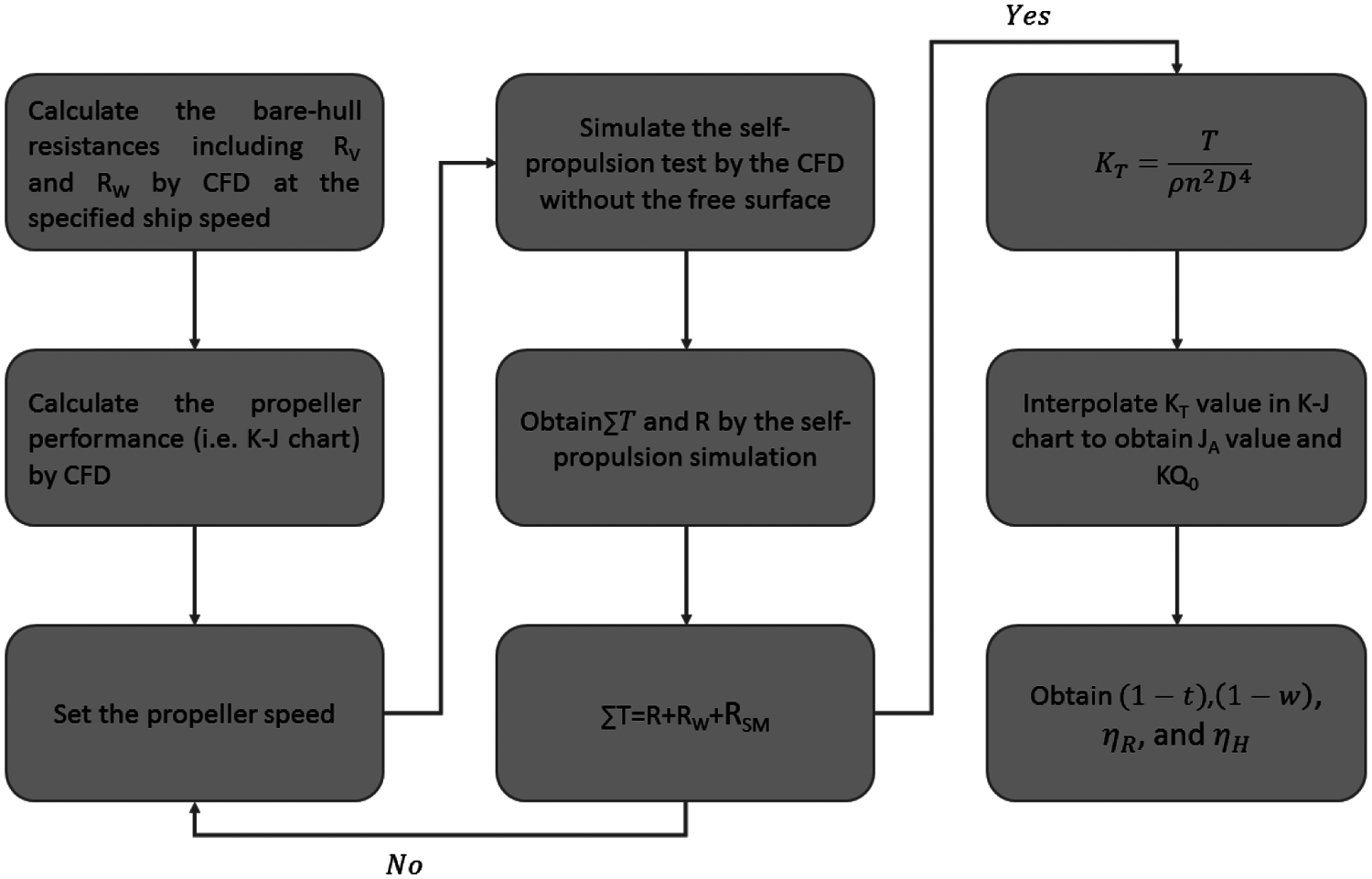
Figure 1: The flowchart for the self-propulsion simulation
The operating propeller and ship hull are both considered in the self-propulsion simulation. It is noteworthy that, in order to save computational time, the free surface is disregarded in the self-propulsion simulation (i.e., disregarding the wave-making resistance (RW)). The value of wave-making resistance (RW) is computed by using the bare hull. In other words, the ship resistance (R) obtained by the self-propulsion simulation only includes the resistance caused by the propeller suction effect (RS) and viscous resistance (RV). Therefore, when the self-propulsion reaches the balance point, the total propeller thrust is equal to the summation of the ship resistance obtained by the self-propulsion simulation (R), the wave-making resistance (RW) and the sea-margin resistance (RSM), as expressed in Eq. (7).
The dimensional formulation and governing equations in this section are referenced in HYKAT HSVA [28].
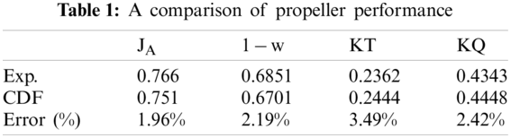
The turbulent model, computing settings and mesh generation used in this study are referred to Kao et al. [10]. Table 1 shows that the predicated results by Kao et al. [10] are in good agreement with the measured values. In other words, the turbulent model, computing settings and mesh generation used in this study are verified.
3 Numerical and Experimental Results
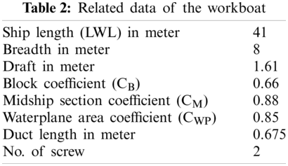
In this paper, an actual two-screw workboat is used as a computing sample. Table 2 shows the related data of the hull geometry.
3.1.1 Hull Viscous Resistance (RV)
This section presents the computation of a single bare hull. The viscous resistance induced by the fluid viscosity, when the hull is advancing, is calculated by the CFD. The computational settings for the bare hull without a free surface are shown in Table 3. As indicated in Table 3, the inflow velocity is 14 (Kn) and the turbulent model is SST k − ω. Fig. 2 presents the flow field of a bare hull without the free surface effect. As shown in Fig. 2, the distance from the inlet to the bow is twice as large as the ship's length (LWL), the distance from the stern to the outlet is three times the ship's length, the distance from the hull to the slip wall is twice if the ship's length, and the ship's length is 41 m. The boundary condition of the inlet is the velocity inlet, that of the outlet is the pressure outlet, and that of the water plane is set as symmetry. The grid independence analysis is shown in Fig. 3. As can be seen, the resistance difference between 7 million meshes and 8.19 million meshes is 0.3%. Thus, 7 million meshes are used in this study to save the computing time, and the obtained viscous resistance is 44917 N.
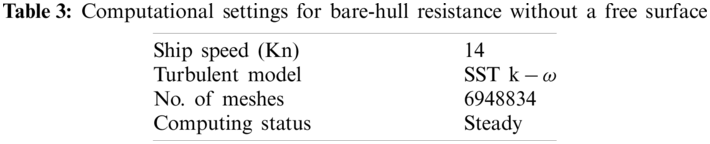
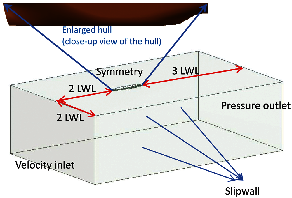
Figure 2: The flow field of a bare hull without the free surface effect
3.1.2 Wave-making Resistance (RW)
This section calculates the bare-hull resistance with the free surface effect. The result is then compared with the result in Section 3.1.1 to obtain the wave-making resistance (RW).

Figure 3: Grid independence analysis of the bare-hull resistance without a free surface
The computational settings for a bare hull with the free surface effect are shown in Table 4. According to the table, the inflow velocity is 14 (Kn) and the turbulent model is SST k − ω. The boundary conditions are listed in Table 5. Fig. 4 presents the flow field of a bare hull with the free surface effect. The trapezoid on the free surface is the region where the grids are refined. In order to shorten the computational time, only half of the hull is calculated and the symmetric boundary condition is applied. The resistance value of the other half of the hull can be obtained by the symmetric boundary condition. The Volume of Fluid model is used to simulate the behavior of waves. The height of the free surface is shown in Fig. 5, and the water surface elevation is set as 1.61 m. Fig. 6 presents the grid independence analysis of the bare-hull resistance with a free surface effect. The resistance difference of the half hull between 4 million meshes and 6 million meshes is less than 1%; it is within the acceptable range. Therefore, 4 million meshes are used in this study for the half hull to obtain satisfactory results and shorten the computational time. In order to describe the wave phenomenon clearly, the Cut-cell meshes are used. The grid arrangements are shown in Fig. 7. The numerical beach is activated at the boundary to avoid the wave reflection at the boundary. The computation in steady state is conduced first to obtain appropriate initial values, and then the transient state is applied. The time step for the transient state is 0.1 sec, and after 4500-step iterations, the resistance value is nearly stable, and there is no obvious jitter. As a result, the average resistance of the half hull from the 4000th step to the 5000th steps is 37.45 KN; thus, the resistance of the entire bare ship with the free surface is 74.9 KN (see Fig. 8). Table 6 compares the experimental result of the bare-hull resistance with the CFD result. As can be seen, the total resistance difference is 4%; it is within the acceptable range.
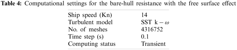
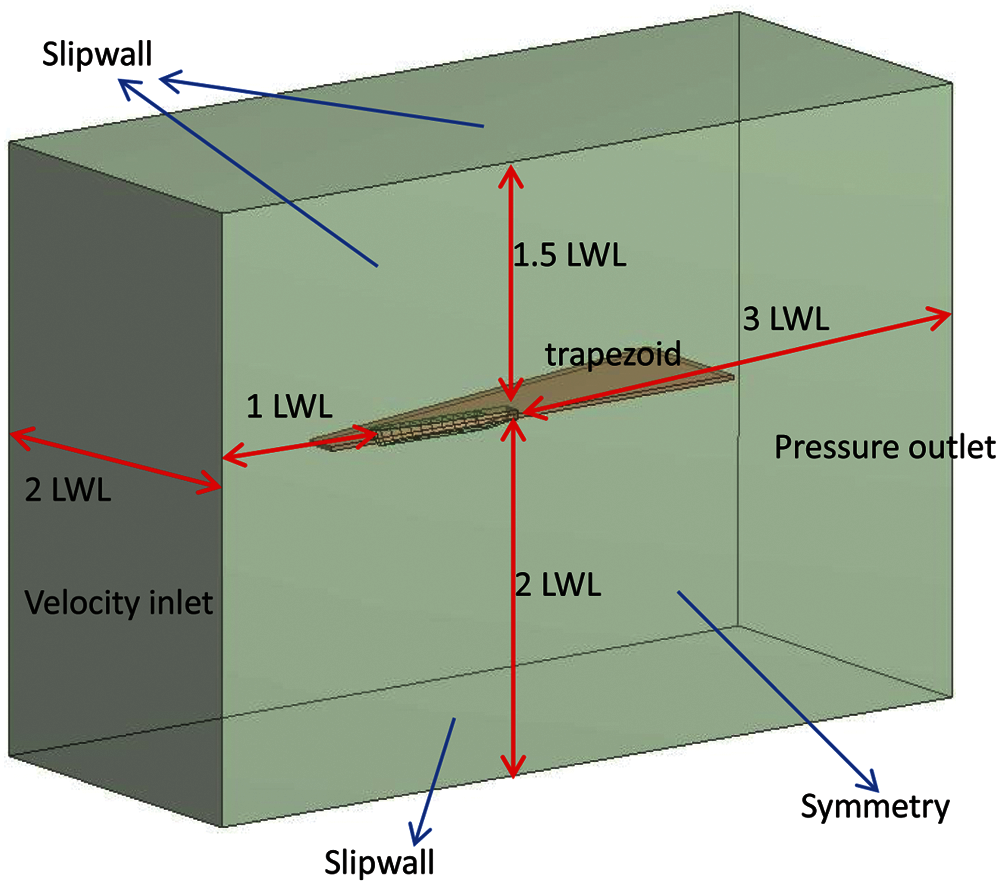
Figure 4: The computing field of the bare hull with the free surface effect
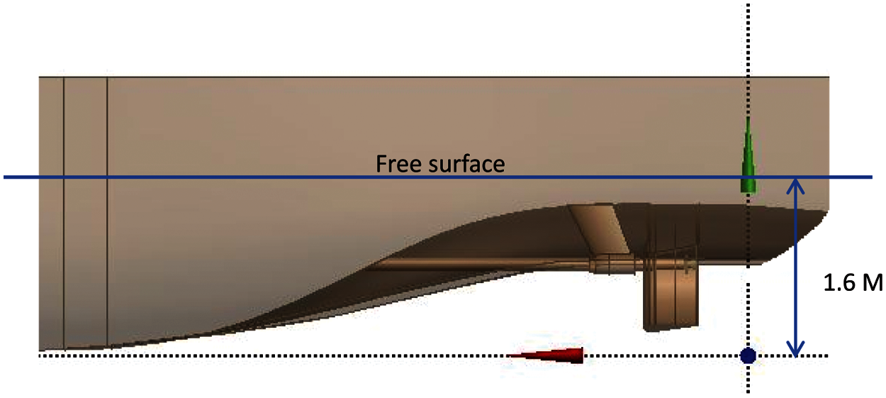
Figure 5: Schematic diagram of the height for the free surface
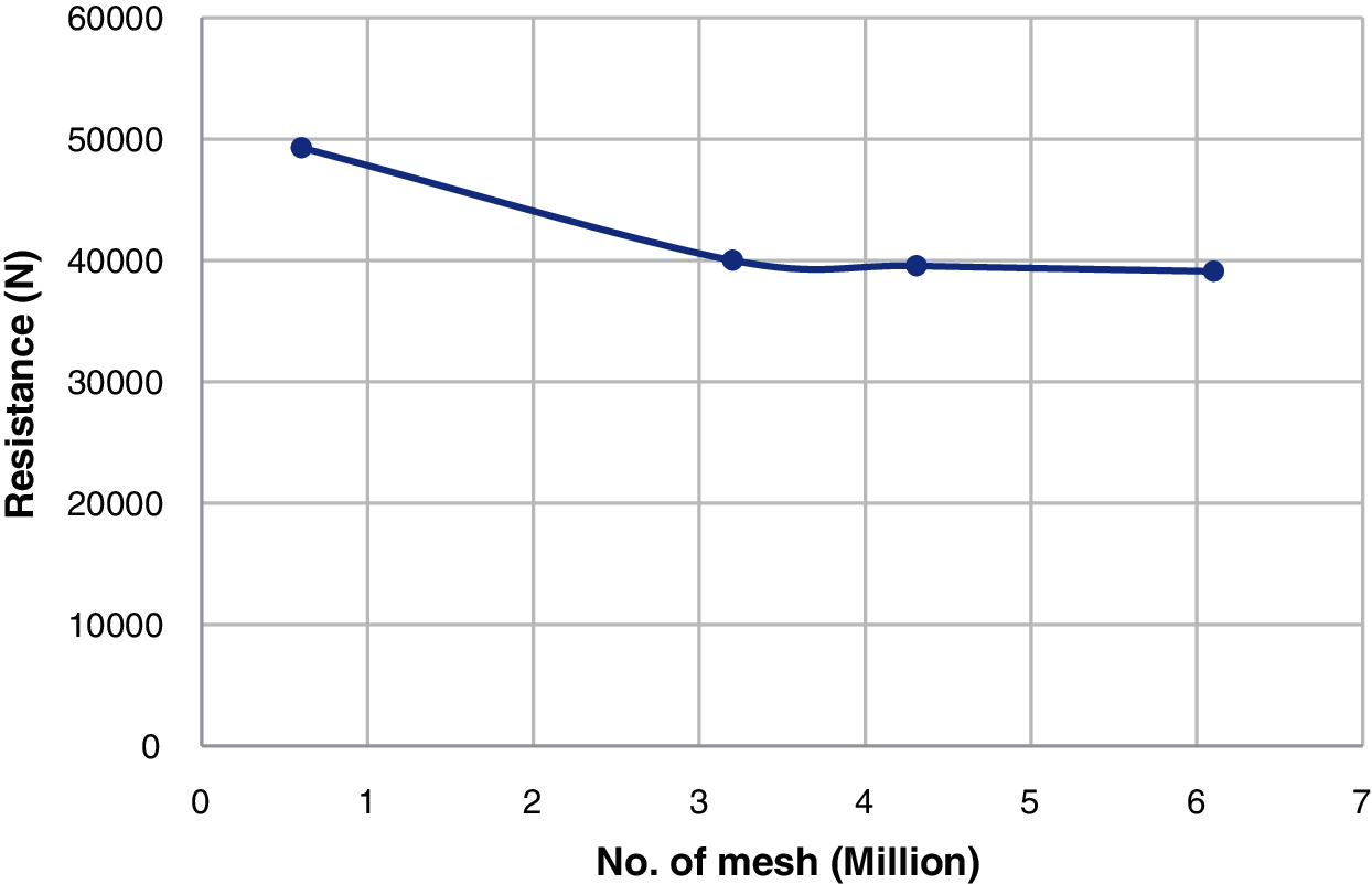
Figure 6: Grid independence analysis of the half bare-hull resistance with the free surface effect
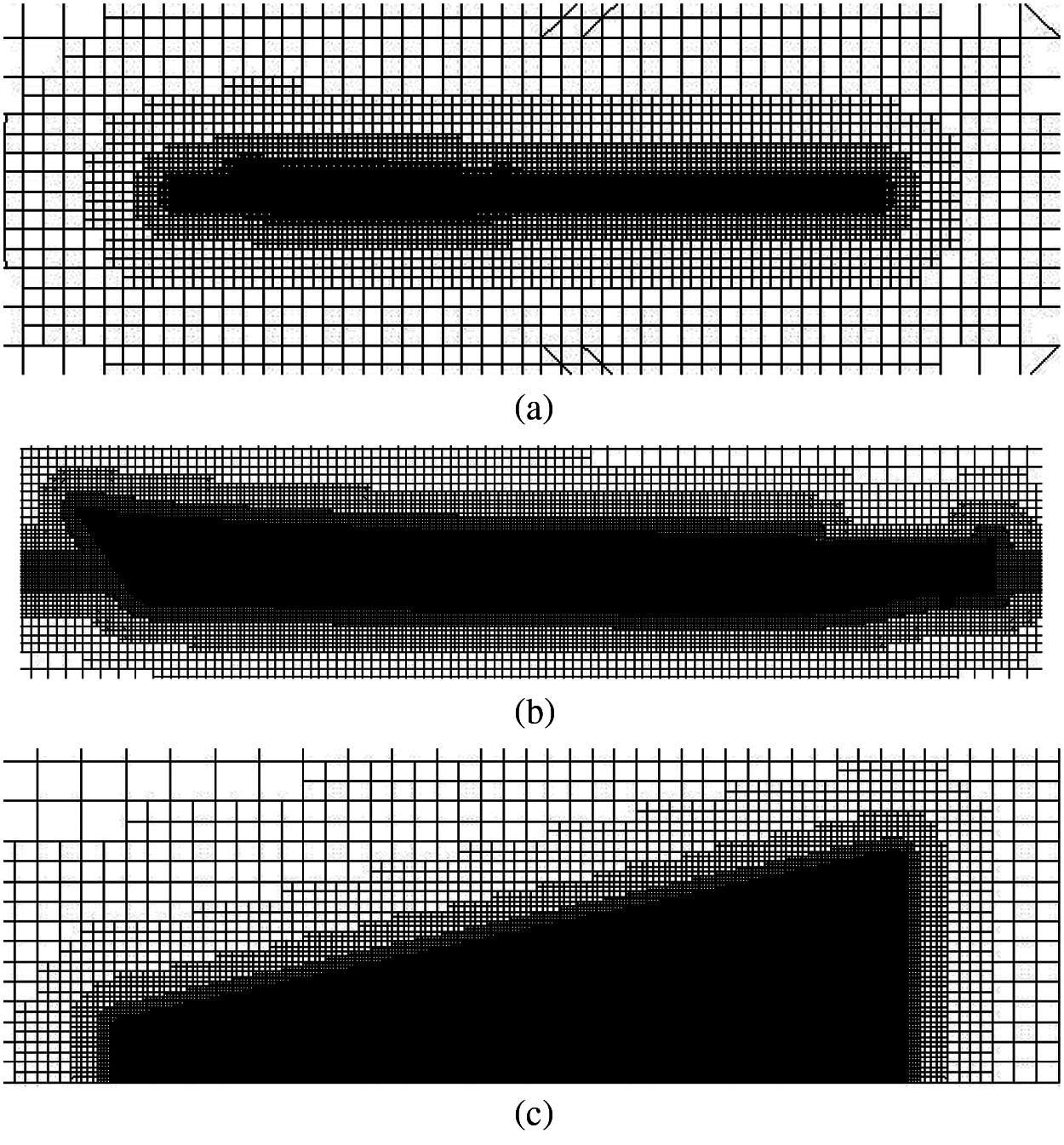
Figure 7: Mesh layout for the flow field of a bare hull with the free surface (a) lateral view of the meshes (b) lateral enlarged view of the meshes (c) top enlarged view of the meshes on the free surface
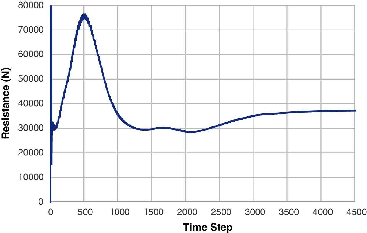
Figure 8: The computing process for the bare-hull resistance with the free surface effect
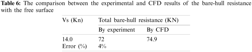
Fig. 9 is the distribution of the wave height. In Fig. 9a, the maximum pressure occurs at the bow stagnation point. Consequently, the waves begin to form near the bow, and a wave crest is generated. The top view of the wave height on the free surface is shown in Fig. 9b. The distribution in Fig. 9b is reasonably similar to the Kelvin wake distribution.
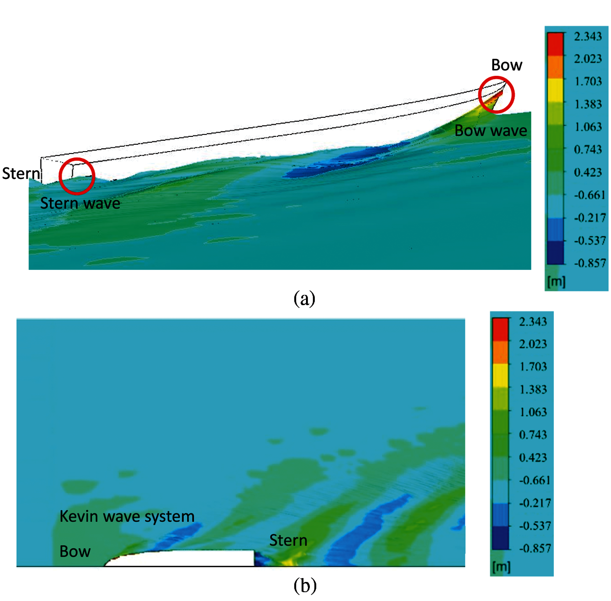
Figure 9: Schematic diagram of the wave height for the free surface (a) lateral view of the wave height of the free surface (b) top view of the wave height of the free surface
3.2 Propeller Performance Curve (K–J Chart)
In addition to the bare-hull resistances described in Section 3.1, the performance curve of the propeller (K–J chart) should be also calculated before the self-propulsion simulation. Table 7 lists the dimensions of the prototype duct and prototype propeller that are used in this paper. Fig. 10 presents the geometries of the prototype propeller and duct. Four combinations of the self-propulsion simulation are calculated in this paper, as shown in Table 8. When the hull is equipped with different versions of the duct and propeller, the thrust and resistance change, and the related propulsion factors have different behaviors.
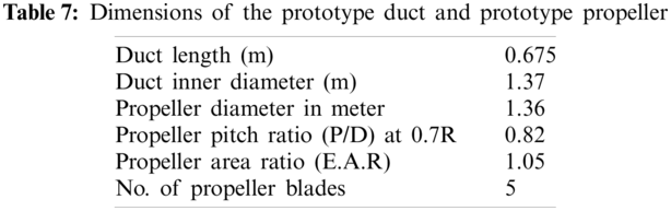
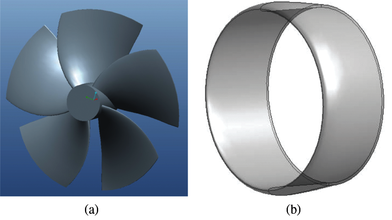
Figure 10: Geometries of the prototype propeller and duct (a) prototype propeller (b) prototype duct
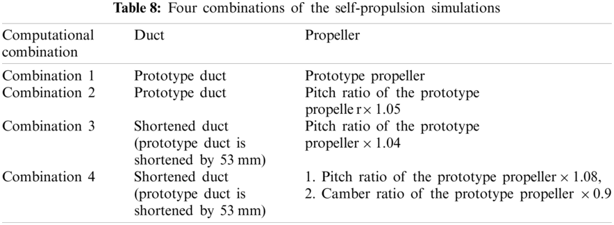
Figs. 11–14 show the K–J charts of the propellers for the four combinations listed in Table 8. For the prototype propeller, the comparison between the predicted values by the CFD and the experimental results is shown in Fig. 11. As can be seen, the calculated results are highly consistent with the experimental values. For the computing sample in this paper, the JA value of the self-propulsion balance point is between 0.6 and 0.7. The difference between the computed and the experimental results for JA = 0.6∼0.7 is very small.
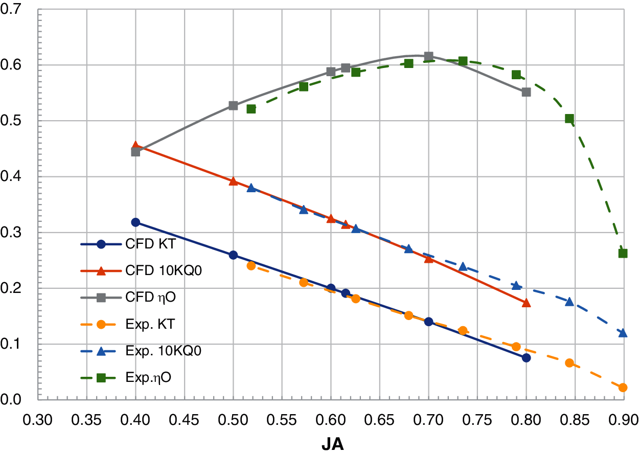
Figure 11: The K–J chart of Combination 1
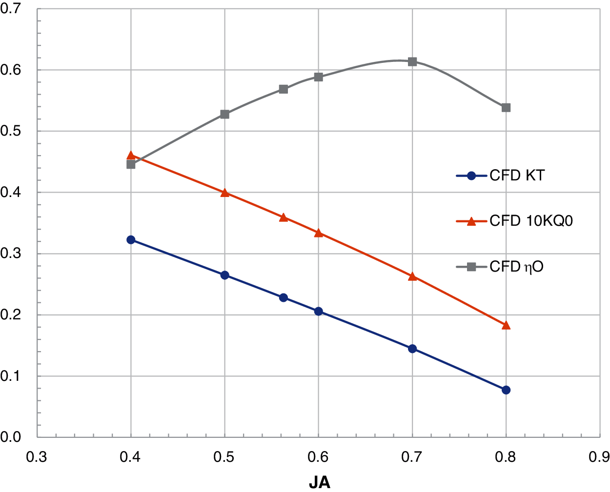
Figure 12: The K–J chart of Combination 2
Figure 13: The K–J chart of Combination 3
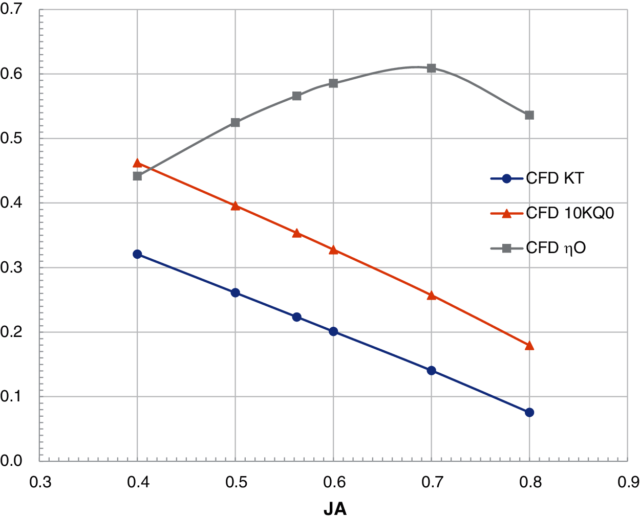
Figure 14: The K–J chart of Combination 4
3.3 Self-Propulsion Simulation
The setting of the computing domains and the mesh generation for the self-propulsion simulations in this paper are based on Kao et al. [10]. Kao et al. [10] applied the CFD for the self-propulsion simulation of the DARPA SUBOFF submarine, and compared the results with the measured results shown in Vaz et al. [6]. The maximum different compared by Vaz et al. [6] was only 3.5%. In addition, the numerical results in Sections 3.1 and 3.2 are compared with experimental values, and the differences are within the acceptable range. Therefore, the correctness of the self-propulsion simulation results in this section can be indirectly confirmed.
Table 9 lists the CFD settings of the self-propulsion simulation. Fig. 15 presents the computing domains of the self-propulsion simulation. As shown in Fig. 15, the number of the meshes in the internal domain is about 4.8 million, and that in the external domain is about 7.2 million. On the external-domain inlet, the steady uniform velocity, Vs, is imposed, the external-domain outlet is set as the pressure outlet, and the free surface is imposed by the symmetry boundary condition. The propeller speed is 10.195 RPS, and the inflow velocity is 14 (Kn). The inclined shaft angle of the propeller is 0.94°.
In Fig. 16, the meshes of the hull, propeller surface and internal domain are refined. Fig. 17 shows the grid independence analysis. The relative difference between the hull resistances (R) calculated by 12 million meshes and 14 million meshes is 1.18%; the relative difference between the propeller thrusts calculated by 12 million meshes and 14 million meshes is 0.1%. Since both differences are within the acceptable range, 12 million meshes are used for the self-propulsion simulations in this paper.
Figure 15: The computing domains of the self-propulsion simulation (a) computing domain for the self-propulsion simulation-external field (b) computing domain for the self-propulsion simulation-internal field (c) enlarged view of stern after combining the internal and external fields
Figure 16: Mesh layout for the self-propulsion simulation (a) enlarged view of the mesh layout near the stern for the self-propulsion simulation (b) enlarged view of the mesh layout in the internal domain for the self-propulsion simulation (c) enlarged view of the mesh layout near the blade tip for the self-propulsion simulation
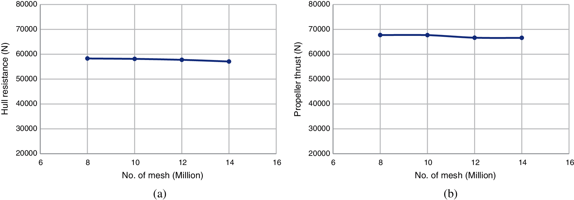
Figure 17: Grid independence analysis of the self-propulsion simulation (a) hull resistance (R) (b) propeller thrust (T)
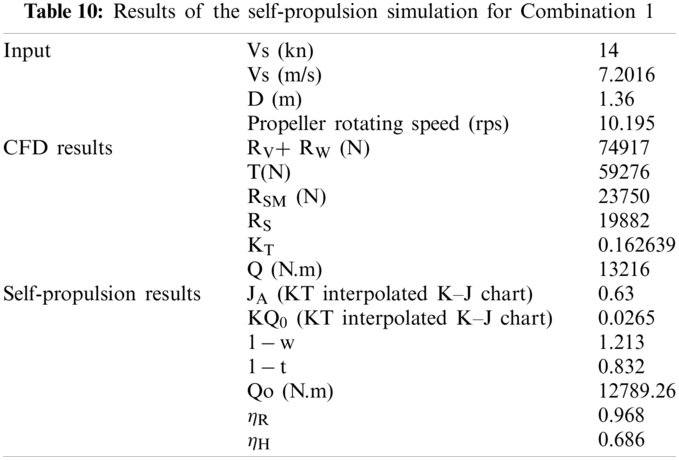
3.3.1 Results of Combination 1
The results of Combination 1 are listed in Table 10. Table 10 indicates that the calculated hull efficiency is relatively low because (1 − w) is too large (i.e., the flow acceleration due to the duct is too significant). Another reason is that the suction effect of the operating propeller on the hull is too large (i.e., the value of (1 − t) is too small). Therefore, the pitch of the prototype propeller in Combination 2 is increased by 5% to increase the thrust coefficient (KT). When the thrust coefficient (KT) is increased, the advanced ratio (JA) and (1 − w) should be decreased (i.e., the propeller loading is increased). Fig. 18 shows the pressures near the stern. When the operating propeller is not included (Fig. 18a), the pressure on the zone marked 1 is 6000–8000 Pa. However, as the operating propeller is considered, the suction effect causes low pressure at the zone marked 3, and the pressure drops to 4000–6000 Pa (i.e., the resistance due to the propeller suction effect is increased). At the zone marked 2, the diffusion effect decreases the flow velocity, thus the pressure is increased. At the zone marked 4, the suction side and the pressure side of the operating propeller result in the apparent pressure junction.
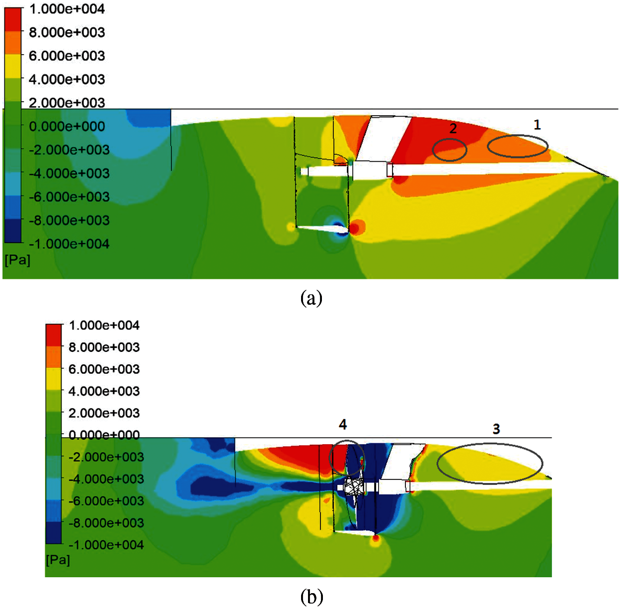
Figure 18: Pressure distribution near the stern for Combination 1. (a) pressure distribution near the stern without an operating propeller (b) pressure distribution near the stern with an operating propeller
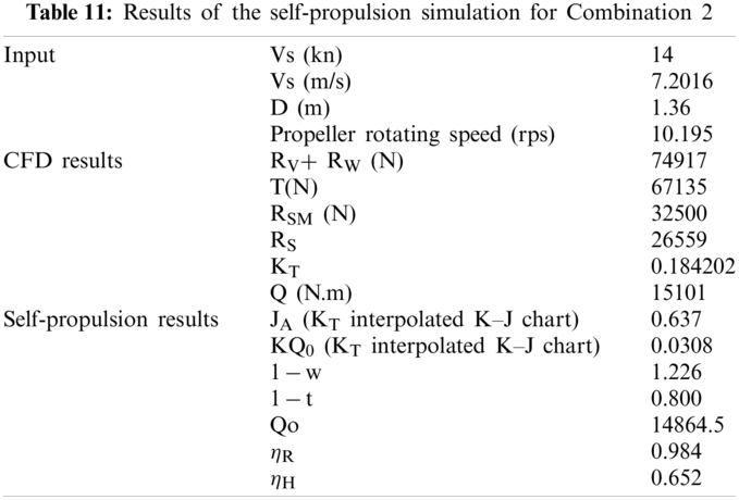
3.3.2 Results of Combination 2
Table 11 indicates the results for Combination 2. According to Table 11, although the thrust coefficient (KT) increases from 0.16 to 0.18 by increasing the pitch ratio, the effective wake of Combination 2 is not expectedly reduced. The reason is that the KT curve in the K–J chart of Combination 2 (Fig. 12) is slightly shifted to the right side as compared with that of Combination 1 (Fig. 12) due to the increment of the propeller pitch. In other words, the interpolated advanced ratio (JA) is increased in Combination 2; therefore, the effective wake is not decreased as expected and hull efficiency is smaller than that of Combination 1.
Fig. 19 presents the pressure distribution near the stern with the operating propeller. In Fig. 19, the zone circled by the red line reveals that the pressure is obviously raised at the six-o'clock position of the propeller pressure side. The pressure difference between the propeller suction and pressure sides becomes larger as compared with Combination 1; consequently, the thrust coefficient is increased. For effectively deducing the acceleration caused by the duct, the duct length is shortened in Combination 3.
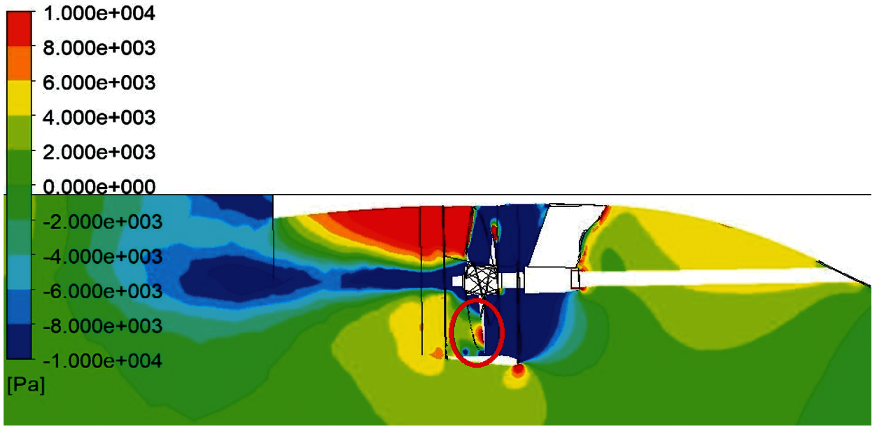
Figure 19: Pressure distribution near the stern with an operating propeller for Combination 2
3.3.3 Results of Combination 3
The results of Combination 3 are shown in Table 12. By comparing the results between Combinations 2 (Table 11) and 3 (Table 12), it is found that (1 − w) is decreased from 1.226 to 1.186 by shortening the duct length (i.e., the propeller inflow VA is decreased). The decrease in (1 − w) leads to a rise in the hull efficiency, ηH. Besides, a decline in the inflow velocity VA results in the less cavitation.
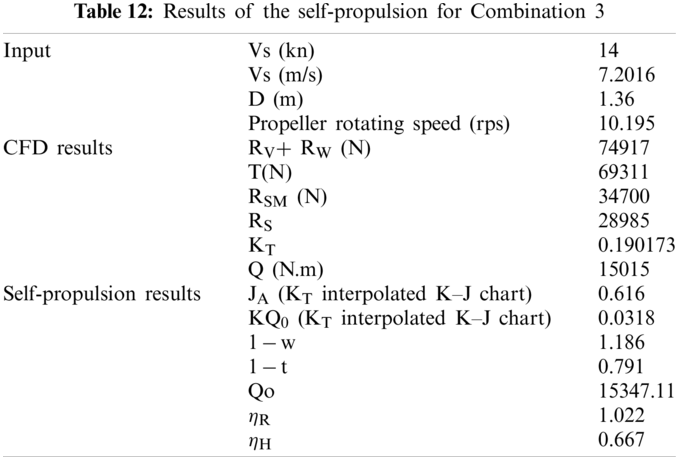
Fig. 20 illustrates the pressure distribution on the leading edge of the foil at 0.8RP (RP the propeller radius) when the propeller blade is at the six-o'clock position (i.e., at the 180-deg position). In Fig. 20, the high pressure is detected on the suction side of the propeller foil. In other words, there is a negative attacked angle for the blade at the six-o'clock position; thus, the face cavitation appears easily. In Combination 4, the propeller pitch is increased to avoid the negative attacked angle.
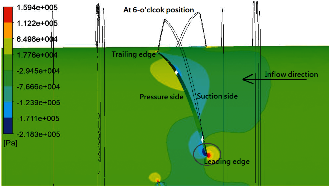
Figure 20: Pressure distribution on the leading edge of the propeller blade for Combination 3 at the six o'clock position
3.3.4 Results of Combination 4
Table 13 presents the results of the self-propulsion simulation for Combination 4. There is only slight difference between the results of Combination 3 and Combination 4. Fig. 21 presents the pressure distribution on the foil at 0.8Rp when the propeller blade is at the six-o'clock position (180° position). As indicated in the circled zone, the negative attacked angle still exists. Fig. 22 illustrates the pressure coefficient (−Cp) distribution of the foil at 0.8Rp as the blade is at different angles (0° and 180°). −Cp is defined by Eq. (8).
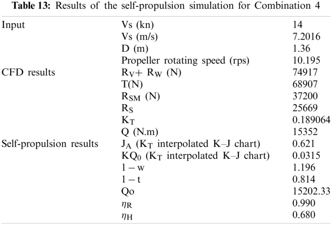
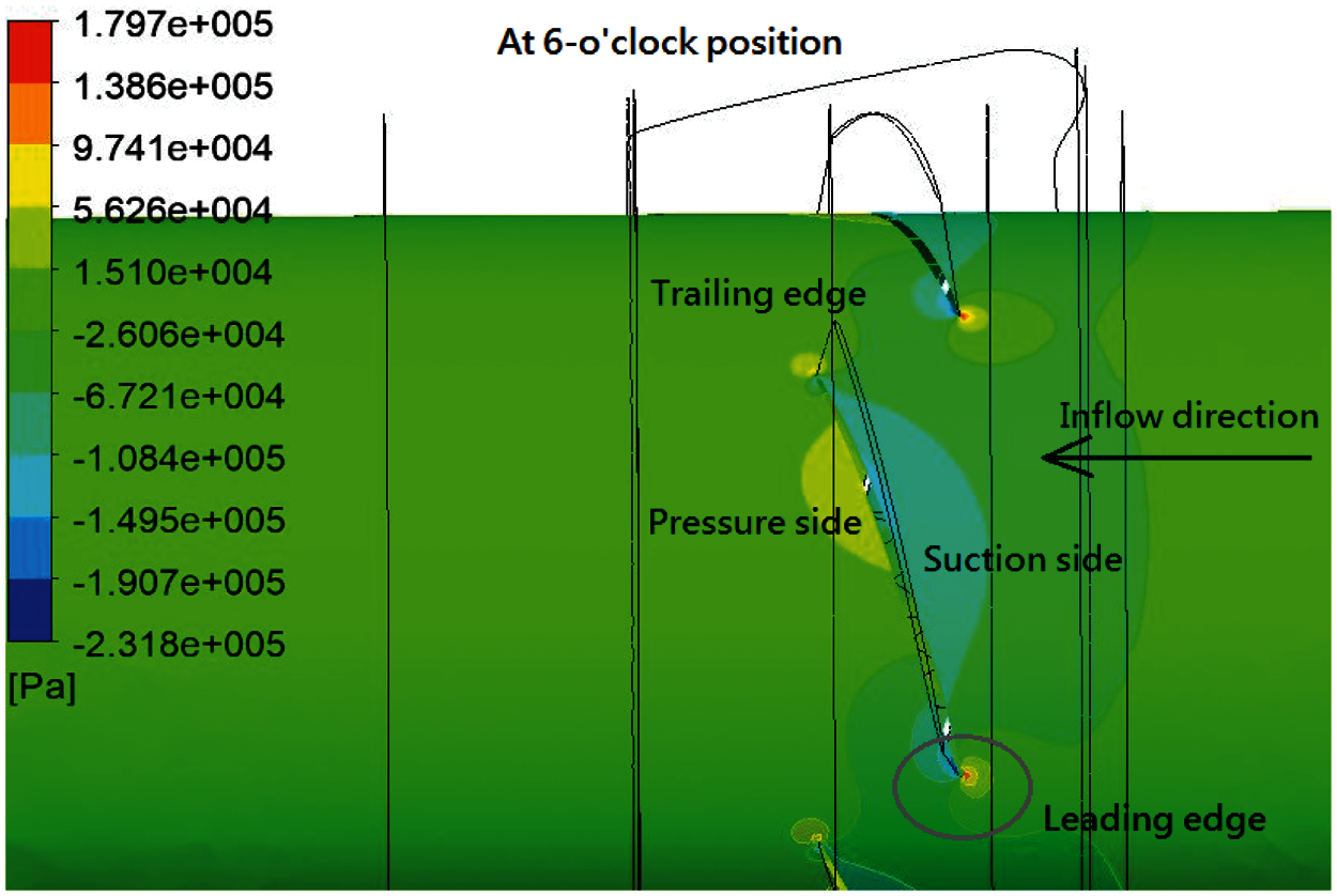
Figure 21: Pressure distribution on the leading edge for the propeller blade for Combination 4 at the six o'clock position
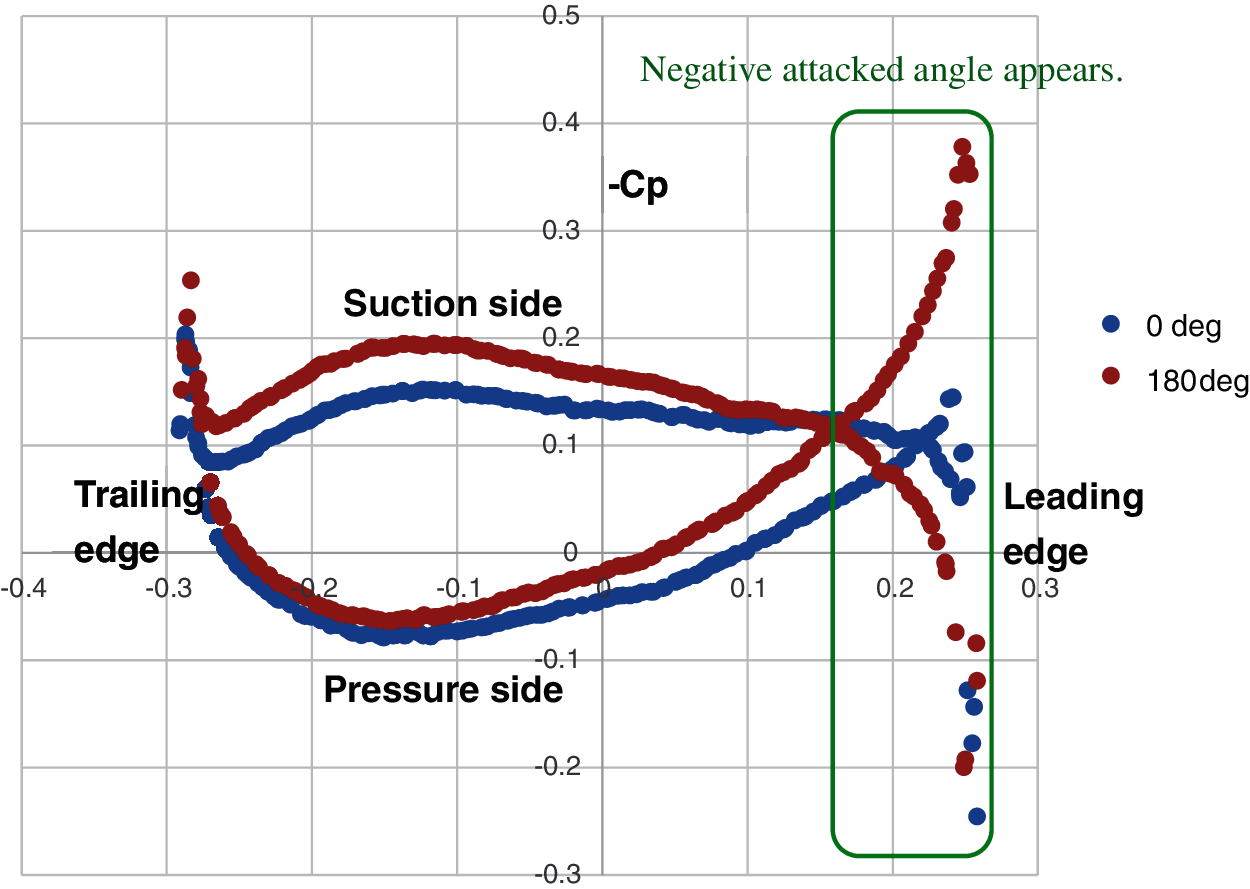
Figure 22: Pressure coefficient (−Cp) distribution on the foil of the 0.8Rp radial position at different blade angles
Here
This study employed CFD to conduct the self-propulsion simulation of a ducted propeller with four combinations of different propeller geometries and duct lengths. The conclusions are as follows:
1. In order to compute the wave-making resistance correctly, the mesh needs to be refined on the free surface. The result is consistent with the Kevin wave system. The maximum pressure occurs at the stagnation point of the bow. Consequently, the waves begin to form, and a wave crest is generated. The results are consistent with the physical phenomenon.
2. The predicted propeller performance curve (K–J chart) and total bare-hull resistance are compared with the experimental results. The comparison comparisons are in good agreement. In other words, the correctness of the self-propulsion simulation is confirmed indirectly.
3. Four combinations with different parameters including the propeller pitch ratio, propeller camber ratio, and the duct length are computed in this paper. These parameters are changed according to the detected results of the fluid acceleration which will affect the propulsive efficiency. As the acceleration is too significant (i.e., the hull efficiency is relatively low, and the face cavitation appears), three strategies are provided to solve this problem according to the propulsive theory. The first strategy is to increase the propeller pitch ratio, the second strategy is to shorten the duct length, and the last strategy is to increase the propeller camber ratio. The computed results show that the most effective way to improve the problem caused by the fluid acceleration is to shorten the duct length for the ducted propulsion system.
4. As the effective wake (1 − w) is too large, the hull efficiency is relatively low. In Combination 2, the pitch of the prototype propeller is increased in order to increase the propeller thrust coefficient and consequently reduce the effective wake. However, the increasing pitch ratio does not work. The KT curve in the K–J chart is slightly shifted to the right side as the propeller pitch is increased. The interpolated advanced ratio (JA) and the effective wake (1 − w) are both therefore increased, and hull efficiency is brought down.
5. The duct is shortened to reduce the duct acceleration effect. As a result, (1 − w) decreases from 1.226 to 1.186 in Combination 3. The hull efficiency is also improved significantly.
6. The propeller inflow is remarkably accelerated by the duct. The strong acceleration causes a negative attacked angle for the propeller; thus, the propeller face cavitation can be detected easily. In the future, it is recommended to redesign the duct geometry for reducing the flow acceleration.
Funding Statement: The authors received no specific funding for this study.
Conflicts of Interest: The authors declare that they have no conflicts of interest to report regarding the present study.
Reference
1. Sung, C. H., Griffin, M., Tsai, J., Huang, T. (1993). Incompressible flow computation of forces and moments on bodies of revolution at incidence. 31st Aerospace Sciences Meeting, pp. 787. Reno, USA. [Google Scholar]
2. Kim, W. J., Kim, D. H., Van, S. H. (2002). Computational study on turbulent flows around modern tanker hull forms. International Journal for Numerical Methods in Fluids, 38(4), 377–406. DOI 10.1002/(ISSN)1097-0363. [Google Scholar] [CrossRef]
3. Huuva, T. (2008). Large eddy simulation of cavitating and non-cavitating flow. Gothenburg, Sweden: Chalmers University of Technology. [Google Scholar]
4. Yang, J., Rhee, S. H., Kim, H. (2009). Propulsive performance of a tanker hull form in damaged conditions. Ocean Engineering, 36(2), 133–144. DOI 10.1016/j.oceaneng.2008.09.012. [Google Scholar] [CrossRef]
5. Toxopeus, S., Vaz, G. (2009). Calculation of current or manoeuvring forces using a viscous-flow solver. International Conference on Offshore Mechanics and Arctic Engineering, 43451, 717–728. DOI 10.1115/OMAE2009-79782. [Google Scholar] [CrossRef]
6. Vaz, G., Toxopeus, S., Holmes, S. (2010). Calculation of manoeuvring forces on submarines using two viscous-flow solvers. International Conference on Offshore Mechanics and Arctic Engineering, vol. 49149, pp. 621–633. DOI 10.1115/OMAE2010-20373. [Google Scholar] [CrossRef]
7. Vaz, G., Jaouen, F., Hoekstra, M. (2009). Free-surface viscous flow computations: Validation of URANS code FRESCO. International Conference on Offshore Mechanics and Arctic Engineering, vol. 43451, pp. 425–437. DOI 10.1115/OMAE2009-79398. [Google Scholar] [CrossRef]
8. Seo, J. H., Seol, D. M., Lee, J. H., Rhee, S. H. (2010). Flexible CFD meshing strategy for prediction of ship resistance and propulsion performance. International Journal of Naval Architecture and Ocean Engineering, 2(3), 139–145. DOI 10.2478/IJNAOE-2013-0030. [Google Scholar] [CrossRef]
9. Korkmaz, K. B. (2015). CFD predictions of resistance and propulsion for the JAPAN Bulk Carrier (JBC) with and without an energy saving device (Master's Thesis). Chalmers University of Technology. [Google Scholar]
10. Kao, J. H., Lin, Y. J., Chin, S. S., Chang, F. N., Tsai, Y. H. et al. (2019). Computational analysis of underwater noise of DARPA SUBOFF submarine. Annual Meeting of Society of Naval and Marine Engineering. Kaohsiung, Taiwan. [Google Scholar]
11. Yu, L., Greve, M., Druckenbrod, M., Abdel-Maksoud, M. (2013). Numerical analysis of ducted propeller performance under open water test condition. Journal of Marine Science and Technology, 18(3), 381–394. DOI 10.1007/s00773-013-0215-4. [Google Scholar] [CrossRef]
12. Yongle, D., Baowei, S., Peng, W. (2015). Numerical investigation of tip clearance effects on the performance of ducted propeller. International Journal of Naval Architecture and Ocean Engineering, 7(5), 795–804. DOI 10.1515/ijnaoe-2015-0056. [Google Scholar] [CrossRef]
13. Gao, D., Su, J., Li, M., Hua, H. (2017). Flow-induced vibro-acoustic analysis of a ducted propeller propulsion system. INTER-NOISE and NOISE-CON Congress and Conference Proceedings, vol. 255, no. 6, pp. 1884–1892. Institute of Noise Control Engineering. [Google Scholar]
14. Gaggero, S., Villa, D., Tani, G., Viviani, M., Bertetta, D. (2017). Design of ducted propeller nozzles through a RANSE-based optimization approach. Ocean Engineering, 145(1), 444–463. DOI 10.1016/j.oceaneng.2017.09.037. [Google Scholar] [CrossRef]
15. Gong, J., Guo, C. Y., Zhao, D. G., Wu, T. C., Song, K. W. (2018). A comparative DES study of wake vortex evolution for ducted and non-ducted propellers. Ocean Engineering, 160(1), 78–93. DOI 10.1016/j.oceaneng.2018.04.054. [Google Scholar] [CrossRef]
16. Andersson, J., Eslamdoost, A., Vikström, M., Bensow, R. E. (2018). Energy balance analysis of model-scale vessel with open and ducted propeller configuration. Ocean Engineering, 167(1), 369–379. DOI 10.1016/j.oceaneng.2018.08.047. [Google Scholar] [CrossRef]
17. Gong, J., Guo, C. Y., Phan-Thien, N., Khoo, B. C. (2020). Hydrodynamic loads and wake dynamics of ducted propeller in oblique flow conditions. Ships and Offshore Structures, 15(6), 645–660. DOI 10.1080/17445302.2019.1663664. [Google Scholar] [CrossRef]
18. Kinnas, S. A., Fan, H., Tian, Y. (2015). A panel method with a full wake alignment model for the prediction of the performance of ducted propellers. Journal of Ship Research, 59(3), 246–257. DOI 10.5957/jsr.2015.59.3.246. [Google Scholar] [CrossRef]
19. Bosschers, J., Willemsen, C., Peddle, A., Rijpkema, D. (2015). Analysis of ducted propellers by combining potential flow and RANS methods. Fourth International Symposium on Marine Propulsors, 39–648. [Google Scholar]
20. Bontempo, R., Cardone, M., Manna, M. (2016). Performance analysis of ducted marine propellers. Part I–Decelerating duct. Applied Ocean Research, 58, 322–330. DOI 10.1016/j.apor.2015.10.005. [Google Scholar] [CrossRef]
21. Bontempo, R., Manna, M. (2018). Performance analysis of ducted marine propellers. Part II–Accelerating duct. Applied Ocean Research, 75, 153–164. DOI 10.1016/j.apor.2018.03.005. [Google Scholar] [CrossRef]
22. Du, W., Kinnas, S. A. (2019). Applying 3D viscous/Inviscid interaction method to predict flows around wings and propellers. SNAME 24th Offshore Symposium, OnePetro. Houston, Texas, USA. [Google Scholar]
23. Villa, D., Gaggero, S., Tani, G., Viviani, M. (2020). Numerical and experimental comparison of ducted and non-ducted propellers. Journal of Marine Science and Engineering, 8(4), 257. DOI 10.3390/jmse8040257. [Google Scholar] [CrossRef]
24. Delouei, A. A., Nazari, M., Kayhani, M. H., Ahmadi, G. (2017). Direct-forcing immersed boundary–non-newtonian lattice boltzmann method for transient non-isothermal sedimentation. Journal of Aerosol Science, 104, 106–122. DOI 10.1016/j.jaerosci.2016.09.002. [Google Scholar] [CrossRef]
25. Karimnejad, S., Delouei, A. A., Nazari, M., Shahmardan, M. M., Rashidi, M. M. et al. (2019). Immersed boundary–thermal lattice boltzmann method for the moving simulation of non-isothermal elliptical particles. Journal of Thermal Analysis and Calorimetry, 138(6), 4003–4017. DOI 10.1007/s10973-019-08329-y. [Google Scholar] [CrossRef]
26. Afra, B., Delouei, A. A., Mostafavi, M., Tarokh, A. (2021). Fluid-structure interaction for the flexible filament's propulsion hanging in the free stream. Journal of Molecular Liquids, 323(3), 114941. DOI 10.1016/.molliq.2020.114941. [Google Scholar] [CrossRef]
27. Patankar, S. V., Spalding, D. B. (1983). A calculation procedure for heat, mass and momentum transfer in three-dimensional parabolic flows. Numerical prediction of flow, heat transfer, turbulence and combustion. 15(10), 54–73. Pergamon. DOI 10.1016/B978-0-08-030937-8.50013-1. [Google Scholar] [CrossRef]
28. HYKAT HSVA (2016). Calm water model tests for a container vessel, Hamburg: Hamburgische Schiffbau Versuchsanstalt. [Google Scholar]
 | This work is licensed under a Creative Commons Attribution 4.0 International License, which permits unrestricted use, distribution, and reproduction in any medium, provided the original work is properly cited. |