Computer Modeling in Engineering & Sciences

DOI: 10.32604/cmes.2022.017669

ARTICLE

Lacunary Generating Functions of Hybrid Type Polynomials in Viewpoint of Symbolic Approach

Nusrat Raza1, Umme Zainab2 and Serkan Araci3,*

1Mathematics Section, Women' s College, Aligarh Muslim University, Aligarh, 202002, India
2Department of Mathematics, Aligarh Muslim University, Aligarh, 202002, India
3Department of Economics, Faculty of Economics, Administrative of Social Sciences, Hasan Kalyoncu University, Gaziantep, TR-27410, Turkey
*Corresponding Author: Serkan Araci. Email: serkan.araci@hku.edu.tr
Received: 29 May 2021; Accepted: 19 August 2021

1  Introduction

Recently, it has been realized that the symbolic method of operational as well as umbral nature provides powerful tool for the study of special functions [1,2]. Babusci et al. [3] developed the formalism of the symbolic method of operational nature for obtaining the generating functions of the Laguerre polynomials. By using symbolic method, the properties of the Laguerre polynomials could have accordingly been reduced to those of a Newton binomial containing an operator treated, in all the manipulations, as an ordinary algebraic quantity. Then Dattoli et al. [4] exploited symbolic method of umbral nature for obtaining the generating functions of the Hermite polynomials.

The Hermite and Laguerre polynomials, being orthogonal polynomial sequences, arise in various fields of engineering, mathematics and physics. The Hermite polynomials have applications in signal processing, probability, combinatorics, numerical analysis, quantum mechanics, random matrix theory, etc. These polynomials are also an example of Appell sequence, which obeys the umbral calculus. The Laguerre polynomials appear in quantum mechanics of the Morse potential, solution of the Schro¨dinger equation for a one-electron atom, oscillator system in phase space and 3D isotropic harmonic oscillator (see [5–8]), etc. The study of Laguerre polynomials becomes more convenient when these are expressed in terms of Laguerre-Wright polynomials. The symbolic method has emerged as a powerful tool to solve the problems involving certain special functions related to different branches of engineering and sciences for example fluid mechanics, physics, engineering and dynamical processes, etc. Most of the special functions do not show certain characteristics by classical methods and hence the importance of symbolic and umbral techniques are realized. These methods are widely used to establish numerous properties such as exponential and ordinary lacunary generating functions, symbolic definitions, symbolic differential equations, symbolic multiplicative and derivative operators etc. of known and new special functions and to evaluate various types of integrals involving these functions. A remarkable application of symbolic method is the convolution of two special functions to introduce and study new special functions. Motivated by the importance and applications of the Hermite and Laguerre-Wright polynomials and the usefulness of symbolic method, in this paper, we introduce and study the Hermite-Laguerre-Wright polynomials using symbolic method.

It has been shown that the concept related to monomiality techniques of the classical and generalized polynomials can be exploited to derive certain properties of families of polynomials, including Hermite and Laguerre polynomials used in pure and applied mathematics see for example [9,10].

The concept and formalism behind the monomiality principle and the symbolic methods can be exploited to introduce certain generalized as well as hybrid special polynomials and functions and to simplify the derivation of the properties of known and newly introduced special functions. The key element of this work is the introduction of the mon-symbolic method, which is the combination of monomiality techniques and symbolic method.

We recall that the ordinary Laguerre polynomials Ln(x) are defined by means of the following series definition [11]:

Ln(x)=n!∑r=0n(−x)rr!2(n−r)!.(1)

Babusci et al. have proved that the symbolic method of defining special functions can be exploited for obtaining several properties of certain special functions, which cannot be easily established by other well known methods [3]. So this method filled a huge vacuum in the study of special functions.

Babusci defined a symbolic shift operator c^z as [3]:

c^zα:f(z)↦f(z+α),(2)

which satisfies the property c^zαc^zβ=c^zβc^zα=c^zα+β. In particular c^zβc^z−β=c^z−βc^zβ=1.

Clearly, for f(z)=1Γ(1+z),

c^zα1Γ(1+z)|z=0=1Γ(1+α).(3)

In view of Eq. (1), the symbolic definition of Ln(x) is given as [3]:

Ln(x)=(1−xc^z)n1Γ(1+z)|z=0.(4)

Interchanging the variables x→y and y→−x in the definition of Laguerre-Wright polynomials [3] the symbolic definition of the 2-variable Laguerre-Wright polynomials (2VLWP) Λn(α,β)(x,y) are as follows [3]:

Λn(α,β)(x,y)=(y−c^zβx)n1Γ(1+z)|z=α,(5)

which on simplifying, gives the following series definition for the 2VLWP Λn(α,β)(x,y) [3]:

Λn(α,β)(x,y)=n!∑r=0n(−x)ryn−rr!(n−r)!Γ(βr+α+1).(6)

The 2-variable associated Laguerre polynomials (2VALP) Ln(α)(x,y) are specified by means of the following series definition [12]:

Ln(α)(x,y)=∑r=0nΓ(1+α+n)(−x)ryn−rr!(n−r)!Γ(1+α+r),

which in view of Eq. (6), gives [3]

Ln(α)(x,y)=Γ(1+α+n)n!Λn(α)(x,y),(7)

where

Λn(α)(x,y):=Λn(α,1)(x,y).(8)

In view of Eqs. (5), (7) and (8), symbolic definition of the 2VALP Ln(α)(x,y) is as follows [3]:

Ln(α)(x,y)=Γ(1+α+n)n!(y−c^zx)n1Γ(1+z)|z=α.(9)

For y = 1, Eq. (5) gives the symbolic definition of the Laguerre-Wright polynomials (LWP) Λn(α,β)(x) in terms of operator c^z is as follows:

Λn(α,β)(x)=(1−c^zβx)n1Γ(1+z)|z=α,(10)

simplifying Eq. (10), we get the following series definition of LWP Λn(α,β)(x):

Λn(α,β)(x)=n!∑r=0n(−x)rr!(n−r)!Γ(βr+α+1).(11)

Next, we recall that the associated Laguerre polynomials (ALP) Ln(α)(x) are defined by the following series definition [11]:

Ln(α)(x)=∑r=0nΓ(1+α+n)(−x)rr!(n−r)!Γ(1+α+r).(12)

In view of Eqs. (11) and (12), we have:

Ln(α)(x)=Γ(1+α+n)n!Λn(α)(x),(13)

where

Λn(α)(x):=Λn(α,1)(x),(14)

which in view of Eq. (10), gives:

Λn(α)(x)=(1−c^zx)n1Γ(1+z)|z=α.(15)

In view of Eqs. (13) and (15), the symbolic definition of the ALP Ln(α)(x) is given as:

Ln(α)(x)=Γ(1+α+n)n!(1−c^zx)n1Γ(1+z)|z=α.(16)

The symbolic definition of the Bessel-Wright function Wβ,α(x) is given as [3]:

W(β,α)(x)=ec^zβx1Γ(1+z)|z=α−1,(17)

which on simplifying, gives the following series definition of Wβ,α(x) [13,14]:

W(β,α)(x)=∑r=0∞xrr!Γ(βr+α).(18)

The symbolic definition of the Mittag-Leffler function Eβ,~α(x) is given as [3]:

Eβ,α(x)=[11−xc^zβ]1Γ(1+z)|z=α−1,(19)

which on simplifying, gives the following series definition of Eβ,~α(x) [13,14]:

Eβ,α(x)=∑r=0∞xrΓ(βr+α).(20)

The study of Hermite polynomials help to solve the classical boundary-value problems in the parabolic regions, through the use of parabolic coordinates and in quantum mechanics as well as in other areas of sciences. We recall that the 2-variable Hermite Kampe de Feriet polynomials (2VHKdFP) Hn(x, y) are defined by means of the following generating function and series definition [15]:

∑n=0∞Hn(x,y)tnn!=exp⁡(xt+yt2)(21)

and

Hn(x,y)=n!∑k=0[n2]xn−2kykk!(n−2k)!,(22)

respectively.

Next, we recall that the nth-order Bessel function Jn(x) is defined by the following series definition [16]:

Jn(x)=∑r=0∞(−1)r(x2)n+2rr!Γ(1+n+r).(23)

In view of Eq. (23) for n = 0, the 0th-order Bessel function Jn(x) is defined as [17]:

J0(2x)=∑r=0∞(−1)rxr(r!)2.(24)

According to the monomi ality principle proposed by Steffensen [18] and developed by Dattoli [10], a polynomial set {pn(x)}n=0∞ is called quasi-monomial if there exist two operators multiplicative operator M^ and derivative operator P^, respectively, such that [10]:

M^{pn(x)}=pn+1(x)(25)

and

P^{pn(x)}=npn−1(x).(26)

The multiplicative operator M^ and derivative operator P^ satisfy the following commutation relation:

[P^,M^]=P^M^−M^P^=1^,

thus, the operatorM^and P^ display a weyl group structure [10]. Several characteristics of polynomial pn(x) can be obtained by using the operators M^ and P^.

Some characteristics are as follows:

(i)   If M^ and P^ have differential realizations, then the polynomial pn(x) satisfy the following differential equation:

M^P^{pn(x)}=npn(x).(27)

(ii)   Assuming here and in the following p0(x) = 1, then pn(x) can be explicitly constructed as:

pn(x)=M^n{1}(28)

(iii)   Consequently the generating function of pn(x) can be obtained as:

exp⁡(tM^){1}=∑n=0∞pn(x)tnn!(|t|<∞).

By induction, Eq. (25) gives:

M^rpn(x)=pn+r(x).(29)

We recall that the 2VHKdFP Hn(x, y) is quasi-monomial with respect to the following multiplicative and derivative operators [10]:

M^H=x+2yDx(30)

and

P^H=Dx,(31)

respectively.

In view of Eq. (22), it can be easily verified that [10]:

Hn(ax,a2y)=anHn(x,y).(32)

Dattoli et al. [4] used the transition of 2VHKdFP Hn(x, y) from monomiality to umbral interpretation. The newton binomial realizes the umbral image of 2VHKdFP Hn(x, y). Dattoli et al. [4] have proved that the operational method become a fairly powerful tool once complimented with a notation of umbral nature. The umbral approach to the 2VHKdFP Hn(x, y) is particularly useful for a straightforward derivation of the relevant properties.

Dattoli redefined the 2VHKdFP Hn(x, y) using umbral approach of symbolic method as [4]:

Hn(x,y)=(x+h^y)nϕ0,(33)

where h^y denotes umbra, which acts on the vacuum ϕ0 in the following manner [4]:

h^yrϕ0=yr2r!Γ(r2+1)|cos(rπ2)|,(34)

which for r = 0, gives ϕ0 = 1. Thus Eq. (33) can be rewritten as:

Hn(x,y)=(x+h^y)n{1}.(35)

In view of Eqs. (28) and (35), we get the following symbolic multiplicative operator of 2VHKdFP:

M^H=(x+h^y).(36)

The use of umbral formalism looks much promising to develop a new technique to study the theory of special polynomials and special functions as well. Hybrid special functions as well as polynomials and their applications has been recognized by Dattoli and his co-workers [2,9,12].

We recall that the 2-variable Hermite-Laguerre polynomials (2VHLP) HLn(x, y) are defined by means of the following series definition [9]:

HLn(x,y)=n!∑r=0n(−1)rHr(x,y)(r!)2(n−r)!(37)

and the Hermite-Bessel-Wright function (HBWF) HWβ,α(x, y) is defined by means of the following series definition [3]:

HW(β,α)(x,y)=∑r=0∞Hr(x,y)r!Γ(βr+α).(38)

Motivated by the work of Babusci and his co-authors on lacunary generating functions for Laguerre polynomials [3] and application of the Laguerre polynomials [12,19,20], in this paper, we introduce certain generating functions for the 2-variable Hermite-Laguerre polynomials and some new families of polynomials. In Section 2, we introduce the Hermite-associated Laguerre polynomials and obtain ordinary generating function via mon-symbolic approach. Further, we define some new families of polynomials such as Hermite-Laguerre-Wright polynomials and find their exponential and ordinary generating functions. In Section 3, we derive the double and the triple lacunary 2-variable Hermite-Laguerre polynomials and find double lacunary generating functions for the 2-variable Hermite-Laguerre polynomials and the Hermite-Laguerre-Wright polynomials. In Section 4, we proposed an idea to find multiplicative and derivative operators for Hermite-Laguerre-Wright polynomials which helps to find symbolic differential equation for the same polynomials.

2  Generating Functions of the Hermite-Associated Laguerre and Hermite-Laguerre-Wright Polynomials

The most interesting example to understand the flexibility and usefulness of the symbolic method is derivation of generating functions of special polynomials and special functions as well. In this paper, we consider two types of generating functions, namely exponential and ordinary.

In this section, we introduce the Hermite-associated Laguerre polynomials and the Hermite-Laguerre-Wright polynomials by using the mon-symbolic method. Also, we obtain certain generating functions of these polynomials.

In view of Eqs. (15) and (36), we introduce the 1-parameter Hermite-Laguerre-Wright polynomials (1PHLWP) HΛn(α)(x,y) by means of the following symbolic definition:

HΛn(α)(x,y):=Λn(α)(x+h^y)=(1−c^zH)n1Γ(1+z)|z=α,(39)

where

c^zH:=c^z(x+h^y).(40)

Since, in view of Eqs. (35) and (40), we have:

c^zHα1Γ(1+z)|z=0=(c^z(x+h^y))α1Γ(1+z)|z=0=Hα(x,y)Γ(α+1)(41)

and

c^zαc^zHβ1Γ(1+z)|z=0=c^zα+βHβ(x,y)1Γ(1+z)|z=0.

Binomially expanding the right hand side of Eq. (39) and then using Eqs. (35) and (40), we have:

HΛn(α)(x,y)=∑r=0n(nr)(−1)rc^zrHr(x,y)1Γ(1+z)|z=α.

Simplifying, we get the following series definition of the 1PHLWP HΛn(α)(x,y):

HΛn(α)(x,y)=n!∑r=0n(−1)rHr(x,y)r!(n−r)!Γ(r+α+1).(42)

Now, in view of Eq. (39), we define the Hermite-associated Laguerre polynomials (HALP) HLn(α)(x,y) by replacing x with (x+h^y) in Eq. (13) as:

HLn(α)(x,y)=Γ(1+α+n)n!HΛn(α)(x,y).(43)

Next, we define the Hermite-Laguerre-Wright polynomials (HLWP) HΛn(α,β)(x,y) by replacing x with (x+h^y) in Eq. (10) as:

HΛn(α,β)(x,y)=(1−c^zβ(x+h^y))n1Γ(1+z)|z=α,(44)

which on using Eq. (35), gives the following series definition of HΛn(α,β)(x,y):

HΛn(α,β)(x,y)=n!∑r=0n(−1)rHr(x,y)r!(n−r)!Γ(βr+α+1).(45)

In view of Eqs. (42) and (45), it is clear that:

HΛn(α,1)(x,y)=HΛn(α)(x,y).(46)

In the recent years, Dattoli used the monomiality principle to find the generating functions for some special polynomials and special functions as well [9–10,12]. Also, Babusci et al. [3] used the concept of symbolic method to find the generating function of the Laguerre Polynomials. In this paper, we combine the symbolic method with the monomiality technique to obtain the generating functions of the HALP HLn(α)(x,y) and the HLWP HΛn(α,β)(x,y).

Now, we establish following result for the ordinary generating function of the HALP HLn(α)(x,y):

Theorem 2.1 The ordinary generating function for HALP HLn(α)(x,y) is given by:

∑n=0,H∞Ln(α)(x,y)tn=1(1−t)(α+1)e−xt1−t+yt2(1−t)2.(47)

Proof. From Eq. (43), we have:

∑n=0H∞Ln(α)(x,y)tn=∑n=0∞Γ(1+α+n)n!HΛn(α)(x,y)tn,(48)

which on using Eqs. (44) and (46) in the right hand side, it gives:

∑n=0H∞Ln(α)(x,y)tn=∑n=0∞Γ(1+α+n)n!(1−c^z(x+h^y))n1Γ(1+z)|z=αtn.(49)

Using the following relation between Gamma function and pochhammer symbol:

(α)n=Γ(α+n)Γ(α)(50)

in Eq. (49), we find:

∑n=0H∞Ln(α)(x,y)tn=Γ(1+α)∑n=0∞(α+1)nn!(t−tc^z(x+h^y))n1Γ(1+z)|z=α,

which on using the following series expansion:

∑n=0∞(α)ntnn!=1(1−t)α,(|t|<1)(51)

gives:

∑n=0H∞Ln(α)(x,y)tn=Γ(1+α)1(1−(t−tc^z(x+h^y)))α+11Γ(1+z)|z=α.

Again, using Eqs. (50) and (51), we have:

∑n=0H∞Ln(α)(x,y)tn=Γ(1+α)1(1−t)α+1∑n=0∞Γ(α+1+n)Γ(α+1)(−t1−t)nc^zn(x+h^y)n1Γ(1+z)|z=α1n!.

Using Eq. (35) in the right hand side of the above equation, we have:

∑n=0H∞Ln(α)(x,y)tn=1(1−t)α+1∑n=0∞(−t1−t)nHn(x,y)n!,

which on using Eqs. (21) and (32) gives assertion (47).

Next, we establish following result for the exponential generating function of the HLWP HΛn(α,β)(x,y):

Theorem 2.2 The exponential generating function for HLWP HΛn(α,β)(x,y) is given by:

∑n=0∞tnn!HΛn(α,β)(x,y)=etHW(β,α+1)(−tx,t2y).(52)

Proof. Using Eq. (44), we have:

∑n=0∞tnn!HΛn(α,β)(x,y)=∑n=0∞tnn!(1−c^zβ(x+h^y))n1Γ(1+z)|z=α=e(1−c^zβ(x+h^y))t1Γ(1+z)|z=α.(53)

From [t,c^zβ(x+h^y)t]=0 and Weyl decoupling identity given by [21]:

eA^+B^=eA^eB^e−k2,k=[A^,B^](k∈C),(54)

We find:

∑n=0∞tnn!HΛn(α,β)(x,y)=ete−c^zβt(x+h^y)1Γ(1+z)|z=α.(55)

Now, expanding the second exponential in the right hand side of the above equation, Eq. (55) yields:

∑n=0∞tnn!HΛn(α,β)(x,y)=et∑r=0∞c^zβr(−t)r(x+h^y)rr!1Γ(1+z)|z=α,

which on simplifying, gives:

∑n=0∞tnn!HΛn(α,β)(x,y)=et∑r=0∞(−t)rHr(x,y)r!Γ(βr+α+1).(56)

Using Eq. (32) in Eq. (56), we have:

∑n=0∞tnn!HΛn(α,β)(x,y)=et∑r=0∞Hr(−xt,yt2)r!Γ(βr+α+1),(57)

which in view of Eq. (38), yields assertion (52).

Since, in view of Eqs. (43) and (46), HΛn(α,1)(x,y)n! := HLn(α)(x,y)Γ(1+α+n).

Therefore, from Theorem 2.2, we get the following result.

Corollary 2.1 The ordinary generating function for the polynomial HLn(α)(x,y)Γ(1+α+n) is given by:

∑n=0∞tnHLn(α)(x,y)Γ(1+α+n)=etHW(1,α+1)(−tx,t2y).(58)

Now, we proceed to obtain the ordinary generating function for the HLWP HΛn(α,β)(x,y). For obtaining the ordinary generating function for the HLWP HΛn(α,β)(x,y), we define the Hermite-Mittag-Leffler function (HMLF) HEβ, α(x, y) by replacing x with (x+h^y) in Eq. (19) as:

HEβ,α(x,y)=[11−c^zβ(x+h^y)]1Γ(1+z)|z=α−1,(59)

which on simplifying and then using Eq. (35), gives the following series definition for the HEβ, α(x, y):

HEβ,α(x,y)=∑r=0∞Hr(x,y)Γ(βr+α).(60)

Now, we establish following result for the ordinary generating function of the HLWP HΛn(α,β)(x,y):

Theorem 2.3 The ordinary generating function for HLWP HΛn(α,β)(x,y) is given by:

∑n=0∞tnHΛn(α,β)(x,y)=1(1−t)HEβ,α+1(−xt1−t,yt2(1−t)2).(61)

Proof. From Eq. (44), we have:

∑n=0∞tnHΛn(α,β)(x,y)=∑n=0∞tn(1−c^zβ(x+h^y))n1Γ(1+z)|z=α,(62)

which on using Eq. (51) for α = 1, gives:

∑n=0∞tnHΛn(α,β)(x,y)=11−t+c^zβt(x+h^y)1Γ(1+z)|z=α,=1(1−t)[1+c^zβt(x+h^y)1−t]1Γ(1+z)|z=α.(63)

In view of Eq. (51) for α = 1, we find:

∑n=0∞tnHΛn(α,β)(x,y)=1(1−t)∑r=0∞c^zβr(−t1−t)r(x+h^y)r1Γ(1+z)|z=α.

Using Eqs. (32) and (35) in the above equation, we have:

∑n=0∞tnHΛn(α,β)(x,y)=1(1−t)∑r=0∞Hr(−xt1−t,yt2(1−t)2)Γ(βr+α+1),

which in view of Eq. (60), gives assertion (61).

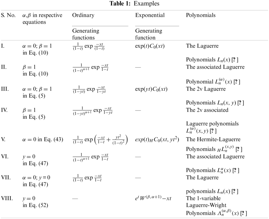
Now, we list the following examples of the special polynomials introduced or discussed in this paper.

In the next section, we obtain the lacunary generating functions of the Hermite-Laguerre polynomials HLn(x, y) and the HLWP HΛn(α,β)(x,y).

3  Lacunary Generating Functions

Babusci et al. redefined the Laguerre polynomials of degrees 2n and 3n (n∈N) by means of the series definitions and obtained the generating functions for these polynomials by using the symbolic method [3]. The generating functions of the Laguerre polynomials of degrees 2n and 3n (n∈N) are named double and triple lacunary generating functions, respectively. Recently, Dattoli et al. [4] obtained the double lacunary generating function of the 2VHKdFP Hn(x, y).

In this section, we define the 2-variable Hermite-Laguerre polynomials HL2n(x, y) and HL3n(x, y) by using the symbolic method. Also, we obtain double lacunary generating functions for the 2VHLP and the HLWP.

In the case when α = 0 in Eq. (43), the associated Laguerre polynomials Ln(α)(x) reduce to the Laguerre polynomials Ln(x) as follows:

HLn(x,y)=HΛn(0)(x,y),

which in view of Eqs. (39) and (40), gives the following symbolic definition of the 2VHLP HLn(x,y):

HLn(x,y)=(1−c^zH)n1Γ(1+z)|z=0.(64)

Now, we give the following theorem for the 2-variable Hermite-Laguerre polynomials HL2n(x, y) and HL3n(x, y).

Theorem 3.1 The series definition for HL2n(x, y) and HL3n(x, y) are given by:

HL2n(x,y)=∑r=0n(nr)(−1)rHχn(r)(x,y)(65)

and

HL3n(x,y)=∑k,r=0n(nr)(nk)(−1)k+rHχn(k+r)(x,y).(66)

Proof. In view of Eq. (64), we have:

HL2n(x,y)=(1−c^zH)2n1Γ(1+z)|z=0,(67)

which on simplifying, gives:

HL2n(x,y)=(1−c^zH)n(1−c^zH)n1Γ(1+z)|z=0=∑r=0n(nr)(−1)r(x+h^y)r(1−c^zH)n1Γ(1+z)|z=r.

Using Eq. (39) in the right hand side of the above equation, we find:

HL2n(x,y)=∑r=0n(nr)(−1)r(x+h^y)rHΛn(r)(x,y).(68)

Therefore, in view of Eqs. (35) and (42), we have:

(x+h^y)rHΛn(r)(x,y)=n!∑k=0n(−1)kHr+k(x,y)k!(n−k)!Γ(k+r+1).

If we denote xrΛn(r)(x) by the polynomial χn(r)(x), then by replacing x with (x+h^y), we find:

Hχn(r)(x,y)=(x+h^y)rHΛn(r)(x,y),(69)

which on using Eq. (39), gives the following symbolic definition of the Hχn(r)(x,y):

Hχn(r)(x,y)=(x+h^y)r(1−c^zH)n1Γ(1+z)|z=r.(70)

Thus, using Eq. (69) in Eq. (68), we get the assertion (65).

By the same way, we can prove it for HL3n(x, y), given by (66).

Now, we proceed to obtain the double lacunary generating function of the 2VHLP HLn(x, y). For this, we denote the product of two 2VHKdFP Hn(x, y) and Hn(z, w), by Hn2(x,y;z,w) which are called Bi-Hermite polynomials.

Thus, in view of Eq. (33), we have:

Hn2(x,y;z,w):=Hn(x,y)Hn(z,w)Hn2(x,y;z,w)=[(x+h^y)(z+h^w)]nϕ0,yϕ0,w.(71)

Now, we define the Bi-Hermite-Bessel function H2J0(x, y; z, w) as:

H2J0(x,y;z,w)=J0(2(x+h^y)(z+h^w))ϕ0,yϕ0,w,

which on using Eq. (24), gives:

H2J0(x,y;z,w)=∑r=0∞(−1)r[(x+h^y)(z+h^w)]r(r!)2ϕ0,yϕ0,w.

In view of Eq. (33), we get the following series definition of H2J0(x, y; z, w):

H2J0(x,y;z,w)=∑r=0∞(−1)rHr(x,y)Hr(z,w)(r!)2.(72)

Now, we are in a position to state the following theorem:

Theorem 3.2 The double lacunary generating function for 2VHLP HLn(x, y) is given by:

∑n=0∞tnn!HL2n(x,y)=etH2J0(x,y;2t,t),(73)

where H2J0(x, y; 2t, t) denotes the Bi-Hermite-Bessel function.

Proof. In view of Eq. (67), we have:

∑n=0∞tnn!HL2n(x,y)=∑n=0∞tnn!(1−c^z(x+h^y))2n1Γ(1+z)|z=0,

which becomes:

∑n=0∞tnn!HL2n(x,y)=et(1−c^z(x+h^y))21Γ(1+z)|z=0.(74)

Simplifying the above equation, we find:

∑n=0∞tnn!HL2n(x,y)=ete−2c^z(x+h^y)t+c^z2(x+h^y)2t1Γ(1+z)|z=0.

Using Eq. (21) in the above equation, we obtain:

∑n=0∞tnn!HL2n(x,y)=et∑r=0∞c^zrr!Hr(−2(x+h^y)t,(x+h^y)2t)1Γ(1+z)|z=0,

which on using Eqs. (32) and (35), it gives:

∑n=0∞tnn!HL2n(x,y)=et∑r=0∞(−1)rHr(x,y)Hr(2t,t)r!2.(75)

In view of Eqs. (72) and (75), we get assertion (73).

Similarly, to obtain the double lacunary generating function for the HLWP HΛn(α,β)(x,y), we define the Bi-Hermite-Wright function (BHWF) H2Wβ,α(x, y; z, w) as:

H2W(β,α)(x,y;z,w)=W(β,α)((x+h^y)(z+h^w))ϕ0,yϕ0,w.

Using Eq. (18) in the right hand side of the above equation, we have:

H2W(β,α)(x,y;z,w)=∑r=0∞[(x+h^y)(z+h^w)]rr!Γ(βr+α)ϕ0,yϕ0,w,

which on using Eq. (33), gives the following series definition of H2W(β,α)(x,y;z,w):

H2W(β,α)(x,y;z,w)=∑r=0∞Hr(x,y)Hr(z,w)r!Γ(βr+α).(76)

We, now state the following theorem:

Theorem 3.3 The double lacunary generating function for HLWP HΛn(α,β)(x,y) is given by

∑n=0∞tnn!HΛ2n(α,β)(x,y)=etH2W(β,α+1)(x,y;−2t,t).(77)

Proof. Using Eq. (44), we have

∑n=0∞tnn!HΛ2n(α,β)(x,y)=∑n=0∞tnn!(1−c^zβ(x+h^y))2n1Γ(1+z)|z=α,

which can be written as:

∑n=0∞tnn!HΛ2n(α,β)(x,y)=et(1−c^zβ(x+h^y))21Γ(1+z)|z=α=ete((−2t)c^zβ(x+h^y)+tc^z2β(x+h^y)2)1Γ(1+z)|z=α,