| Computer Modeling in Engineering & Sciences |
DOI: 10.32604/cmes.2022.016779
ARTICLE
CFD-Based Evaluation of Flow and Temperature Characteristics of Airflow in an Aircraft Cockpit
Key Laboratory of Industrial Design and Ergonomics, Ministry of Industry and Information Technology, Northwestern Polytechnical University, Xi'an, 710072, China
*Corresponding Author: Suihuai Yu. Email: ysuihuai@vip.sina.com
Received: 25 March 2021; Accepted: 01 September 2021
Abstract: The rational design of airflow distribution is of great importance for comfort and energy conservation. Several numerical investigations of flow and temperature characteristics in cockpits have been performed to study the distinct airflow distribution. This study developed the coupled heat transfer model of radiation, convection, and heat conduction for the cockpit flight environment. A three-dimensional physical model was created and a shear stress transfer (SST) k-w turbulence model was well verified with a high prediction accuracy of 91% for the experimental data. The strong inhomogeneous flow and temperature distribution were captured for various initial operating conditions (inlet temperature, inlet pressure, and gravitational acceleration). The results indicated that the common feature of the flow field was stable in the middle part of the cockpit, while the temperature field showed a large temperature gradient near the cockpit's top region. It was also found that there was remarkable consistency in the distributed features, regardless of the applied initial operating conditions. Additionally, the mass flux and the top heat source greatly affected the flow and temperature characteristics. This study suggests that an optimized operating condition does exist and that this condition makes the flow and temperature field more stable in the cockpit. The corresponding results can provide necessary theoretical guidance for the further design of the cockpit structure.
Keywords: Aircraft cockpit; airflow distribution; flow characteristics; temperature characteristics; inhomogeneous behaviors
| Nomenclature | |
| Cp | specific heat |
| G, g | gravitational acceleration |
| Gs | absorption coefficient |
| T | temperature |
| Reynolds stress | |
| Pk | turbulent generation term |
| R | inhomogeneity coefficient |
| U0 | buoyancy velocity |
| X | x axis |
| y | y axis |
| y+ | wall distance in conventional wall unit |
| z | z axis |
| Greek symbol | |
| σ | Stefan-Boltzmann constant |
| αs | solar incoming radiation |
| β | volume expansion coefficient |
| δ | kronecker delta |
| ɛ | emissivity |
| λ | thermal conductivity |
| μ | viscosity |
| μt | turbulent viscosity |
| v | molecular viscosity of fluid |
| ρ | density |
| Subscripts | |
| ave | average |
| b | bulk |
| c | cold wall |
| f | fluid |
| h | hot wall |
| in | inlet |
| max | maximum |
| min | minimum |
| out | outlet |
| w | wall |
Confined turbulent flow is of great importance for a variety of practical engineering applications, such as air conditioning for cooling micro-electronic devices, air supply in buildings, and airflow in vehicles and aircraft cockpits [1,2]. Among these applications, the airflow distributions in cockpits are more confined and complex compared with airflow distributions in indoor environments and buildings [3–5]. In a cockpit, the airflow may be more sensitive to the structure design and the air supply system, which has a great effect on user experience, especially during long flights [6–8]. Hence, the potential flow characteristics of the airflow in the indoor environment of a cockpit appear crucial. In general, a well-designed airflow should retain a small temperature difference in vertical space. Hence, temperature characteristics also need to be carefully studied and evaluated to increase our understanding of temperature distribution in a cockpit.
At present, two main methods are available for investigating the flow and temperature distribution in a cockpit, i.e., experimental measurements and numerical simulations. However, there are extremely few studies on aircraft cockpits. In this study, the distinct flow and temperature characteristics in an aircraft cabin are investigated. In terms of experimental approaches, there are several classical research studies. In general, flows in cockpits are in a low-speed turbulent state, and experimental data are obtained with high measurement accuracy. For the investigation of airflow features, tests have been performed to characterize the airflow distribution [9–11], flow characteristics [12–14], and temperature characteristics [13,15,16]. During the airflow transport, the temperature distribution has also been evaluated. Zhang et al. [17] experimentally measured the air velocity and temperature distribution. Li et al. [18] evaluated the inhomogeneous distribution pattern of temperature in a selected complex narrow space. They found that the velocity and temperature features were greatly affected by the initial air volume. The aforementioned experimental results have indicated that the air environment is very important for user comfort and that the air environment can also be improved by reasonable airflow distribution. Most of the experimental measurements were carried out in an actual stationary aircraft, which was because an in-flight measurement would be very expensive as it would need to be conducted within a reasonable requirement of spatial resolution. Because the airflow is unsteady, measuring the flow and temperature fields poses an enormous challenge. The specific coupled heat transfer model for the cockpit in flight is still unknown. Thus, it is necessary to study the flow and temperature characteristics in a cockpit under various operating conditions.
Compared with experimental methods, computational fluid dynamics (CFD) is a potential numerical tool that is less expensive and more efficient. Consequently, airflow can be predicted and can contribute to structural optimization and cockpit design with respect to the comfort requirements. Danca et al. [19] numerically investigated air distribution and temperature characteristics, and they presented numerical simulations to verify the feasibility and effectiveness of the scheme. Yao et al. [20] developed an anisotropic model based on the basic V2f turbulence model, and the results indicated that the new model could successfully reproduce the flow instability characteristics. You et al. [21] used the measured data to evaluate the prediction performance of a renormalization group (RNG) k-e and SST k-w turbulence model. The results indicated that the SST k-w model was better than the RNG k-e model in predicting airflow distribution. Lin et al. [22,23] identified distributional features of airflow in terms of flow and temperature. They calculated the flow and temperature information using both large eddy simulation (LES) and Reynolds-averaged Navier-Stokes (RANS) turbulence models. At present, CFD has been adopted extensively in the studies of air-supply design [24–26], flow and temperature characteristics [27,28]. Qian et al. [29] used CFD and the Wells-Riley equation to capture a spatial flow distribution. Zhang et al. [30] focused on the existing temperature distribution and found that the fluid concentration showed an inhomogeneous behavior. However, as these turbulence models adopted approximations in CFD, the corresponding numerical results remain uncertain, and the existing thermo-fluid boundary conditions have not been carefully considered. Additionally, few studies have focused on the inhomogeneous behaviors that exist with the changes in the flight models.
This study establishes a three-dimensional cockpit model with various thermo-fluid boundaries, and evaluates the distinct flow and temperature characteristics with the commercial software Fluent 19.0. In addition, the effects of the various boundary conditions on the inhomogeneous behaviors are extensively analyzed.
2 Geometrical Models and Boundary Conditions
The flow and temperature field are the dominant factors influencing the driving performance and comfort of a cockpit. The airflow in a cockpit is a complex three-dimensional flow interaction. The simulation object in this research is an internal flow field that is solved with CFD equations, as well as the boundary conditions on the walls. Fig. 1 illustrates the flowchart of modeling processes. It mainly includes four parts: heat transfer model, turbulence model, geometric model and CFD analysis. Fig. 2 shows the schematic diagram of the cockpit space with a complex structure.

Figure 1: Flow diagram of modeling process

Figure 2: Schematic diagram of the space configuration in the cockpit with (a) cockpit canopy and (b) internal flow field and the cockpit structure
For the duration of the simulated flight, different classification stages are extracted, summarized, and grouped, as shown in Fig. 3. Each phase of the flight stage is described as follows:
• Slipping out: Flight moves the blocks from the initial position to the runway
• Run-up: Without brakes
• Takeoff: Flight is 35 ft above the ground
• Climbing: Flight is 35–20000 ft above the ground
• Cruise: Flight is operated at an altitude averaging 20000 ft in a stable state
• Drop-in: Flight is at any altitude between 20000 and 1500 ft
• Waiting: Gliding at the same altitude
• Approaching: Flight is 1500–100 ft above the ground
• Landing: Ground-contact stage
• Buffer: Brake starting and buffering
• Slipping in: Moving the flight to a target position
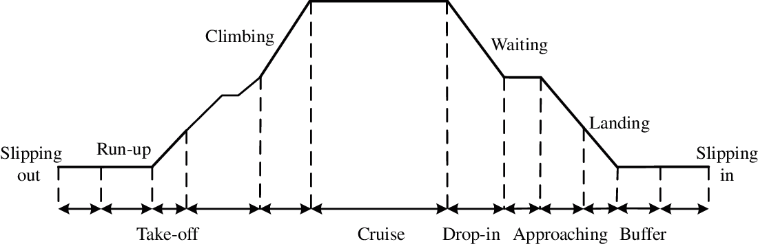
Figure 3: Different phases during the flight
It is worth noting that when the flight is at the climbing and dropping stages, the various accelerations are considered the maximum feature. The flight undergoes a non-linear acceleration that is mainly attributed to the flight climbing and dropping speed. This results in the distinct inhomogeneous behaviors in the cockpit space for different flight acceleration effects, which are focused on and evaluated in this study.
The associated boundary and initial conditions are shown below. As shown in Fig. 4, supply air is sent into the cockpit by the air distribution ventilation system. Hence, the flow and temperature fields are formed in accordance with the changes of the inlet air. The initial parameter control, such as the inlet temperature and mass flux, should be considered for the further construction design of the supply air system. In particular, the existing mixed thermal boundary condition needs to be carefully considered inside the cockpit canopy because the convective and radiation heat transfer may partly act on the canopy wall.
Fig. 5 shows the schematic diagram for developing heat transfer model. The whole heat transfer processes strictly obey the energy conserving law. The solar incoming radiation is the heat source, which flows into convection heat transfer, radiation heat transfer and heat conduction. Because only the fluid field inside the cockpit is studied, we completely convert the radiation term through the canopy into a thermal load term. We treat the cockpit as an approximate plane that exchanges heat between the inner and outer walls. The significant inner wall temperature can be obtained with the following formula [31,32]:
where Gs and αs are the solar incoming radiation and absorption coefficients, respectively; hin and hout are the convective heat transfer coefficients on the inner and outer walls of the canopy wall, respectively; ɛ is the emissivity and σ is the Stefan-Boltzmann constant of 5.672 × 10⁻⁸ W/m2⋅K; Tw, in and Tw,out are the inner and outer wall temperatures, respectively; Tf, in and Tf,out are the inner and outer air temperatures, respectively; λ is the thermal conductivity coefficient; and δ is the thickness of the cockpit. Based on [31], the flight speed is less than 2 Ma, under which the radiation term σɛ(Tw,out--Tf,out) can be ignored when compared with the inside convective heat transfer. Thus, a new mixed heat transfer formula can be obtained with Eqs. (1) and (2).

Figure 4: Schematic diagram of the ventilation system with (a) supply air system and (b) exhaust air system
According to data reported in [31,32], when the flight altitude is between 35 and 20000 ft, the significant parameters are listed in Table 1. The fact that the space of the cockpit is small and confined, along with the complex structure, makes the flow analysis very valuable. The primary purpose of the present study is to establish a flow and heat transfer mode, which is numerically integrated with CFD tools in the cockpit domain. The boundary conditions are shown in Table 2, with the supply air set as an inlet boundary and the outlet boundary defined as outflow. It is noteworthy that the acceleration ranges from 1 to 4 g, and the acceleration is bound to cause the inhomogeneous behaviors, which will be evaluated and analyzed.

Figure 5: Schematic diagram for developing heat transfer model. (a) The thermal boundary conditions. (b) Heat transfer and exchange processes


The cockpit is an air-filled space where is characterized by the distinct inhomogeneous flow and temperature distribution. Before implementing the numerical simulation, the physical properties must be determined to be input into the FLUENT software. Thermo-physical properties, i.e., specific heat (cp), thermal conductivity (λ), density (ρ) and viscosity (μ), are considered the most important input parameters. According to [31], the analysis of thermo-physical properties is carried out by assessing the basic trend.
As shown in Fig. 6, the specific heat (cp) and thermal conductivity (λ) exhibit an increasing trend, whereas the density shows a decreasing trend. In principle, thermo-physical property of air fluid could be highly affected by flow and temperature redistribution in cockpit. The values of the density and viscosity for the temperature ranging from 283 to 313 K are listed in Table 3, with reference to which, the significant thermo-physical properties can be input into the FLUENT 19.0 platform.

Figure 6: Trend with air temperature for (a) special heat, (b) thermal conductivity, and (c) density. Data are taken from the [31]

Inhomogeneous behaviors are ubiquitous in nature. The effect of unresolved scales must be taken into account to recover a reliable description of motion. Currently, numerical methods are categorized into three classes, i.e., Reynolds-averaged Navier-Stokes (RANS), large eddy simulation (LES), and direct numerical simulation (DNS). DNS and LES are suitable for solving for tiny vortex and turbulence statistics in all scales [25], with an obvious drawback in the demand for very high-quality mesh. The RANS model with time-averaged equations is mostly used to simulate practical flows in which various turbulence models play a key role [26]. Moreover, the predictive ability of the RANS model is valid for practical engineering requirements, and the model parameters are fitted to experimental or simulation data in various conditions. With comprehensive consideration, the RANS model is adopted in this study. To obtain accurate results, it is necessary to verify that the proposed RANS turbulence model achieves a better predictive performance for the flow and temperature characteristics. In particular, the various gravitational accelerations are bound to generate distinct buoyancy-driven flow that further induces notable inhomogeneous flow behaviors in the cockpit. Thus, a complex flow field can be predicted, which also increases the difficulty of the turbulence validation.
The classical models, i.e., Transition k-kl-w, SST k-w, Standard k-e, Realizable k-e, Reynolds stress, Transition SST, and v2f, are employed to analyze significant differences for the predictive inhomogeneous behaviors. Tian et al. [33] have analyzed the inhomogeneous flow and temperature behaviors. The schematic view of the three-dimensional space of the flow field is shown in Table 4. The length, width, and height of the physical space are 1.45, 0.725, and 0.725 m, respectively. The temperature difference between the hot source temperature (Th = 333.15 K) and the cold source temperature (Tc = 293.15 K) induces the thermal stratification phenomenon, which aggravates the formation and development of inhomogeneous flow behaviors. To validate the prediction model, a joint assessment of the flow and temperature information is required. Hence, a dimensionless temperature (T--Tc/Th--Tc) and buoyancy velocity (U0 = (gβΔTH)1/2) are defined. The detailed description is shown in Table 4. It should be noted that the central plane x = 0.3625 m is perpendicular to the x-axis, and this plane bisects the space. In my study, this central plane is adopted to derive the dimensionless temperature (T--Tc/Th--Tc) and the buoyancy velocity (U0 = (gβΔTH)1/2).

The results are shown in Fig. 7. It can be clearly observed that the experimental data are more variable, particularly in the near-wall region where the best performing validation region is. Thus, broadly speaking, a turbulence model is excellent if it is within some model-error-informed tolerance (a prediction accuracy greater than 90%, or approaching 100%, indicates an outstanding model). Clearly, the Standard k-e (2 eqn), Reynolds stress (7 eqn), and v2f (4 eqn) are less effective for the ux/U0 prediction in the near-wall region, as their prediction accuracies are 81%, 82%, and 83%, respectively. This means that the selected turbulence model with two equations may not well capture the fundamental flow properties or reflect the basic mechanical law of viscous fluid flow. The larger error is equally likely to appear for Realizable k-e, Transition SST, and Transition k-kl-w, with prediction accuracies of 69%, 76%, and 77%, respectively. Fortunately, the SST k-w model, rather than others, gives the best-predicted trend that is similar to the experimental data. The prediction accuracy of the SST k-w model reaches 91%, which achieves excellent model applicability.
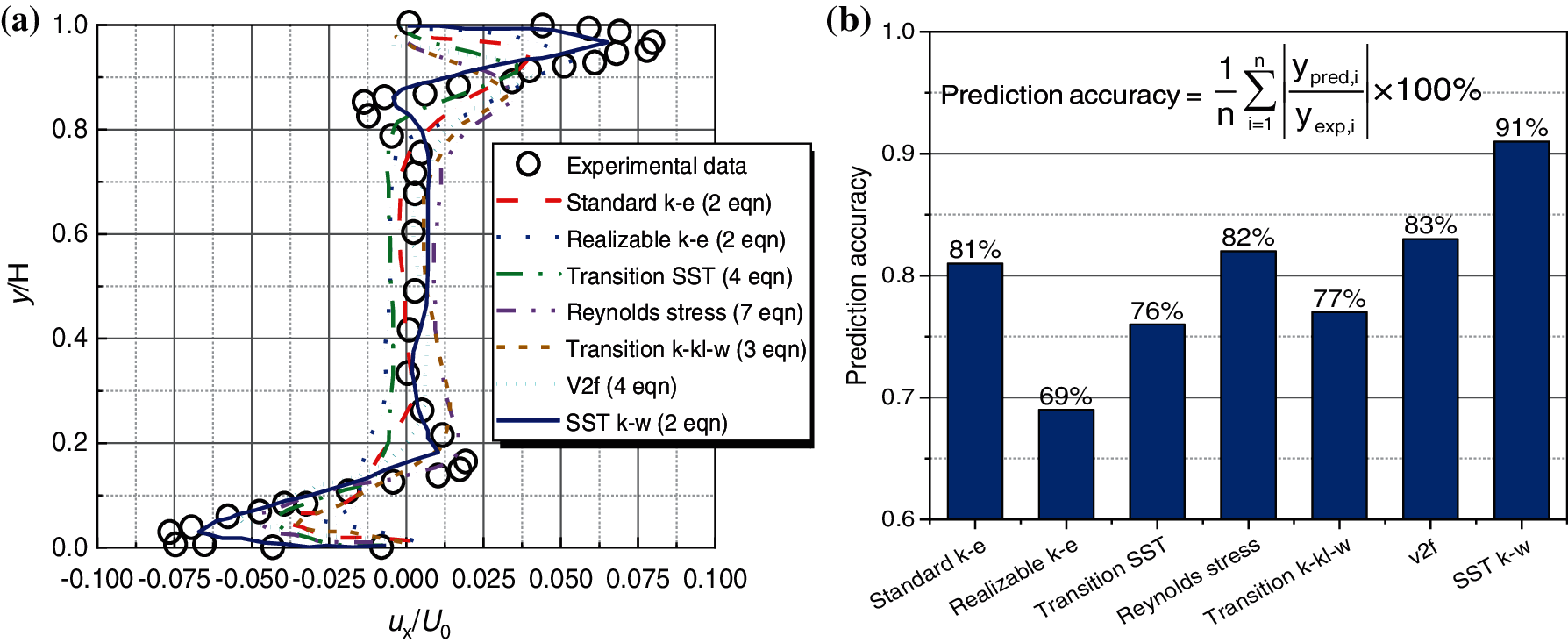
Figure 7: Validation of turbulence model under inhomogeneous velocity distribution conditions: (a) comparison between the experimental data and the numerical results; (b) comparison of prediction accuracy based on different turbulence models; here, n representing the number of experimental data points, “pred” and “exp” denoting the predicted and experimental values, respectively. Experimental data are taken from the [33]
In practical conditions, the cockpit is characterized by inhomogeneous behaviors that are induced by the large temperature gradient. Based on the validation results, the SST k-w model can reliably capture more turbulent features and scales. Thus, based on the above analysis, the SST k-w model achieves the best predictive ability, even for the inhomogeneous and buoyancy conditions.
The numerical simulation of flow and temperature distribution in cockpit is performed using commercial software Fluent 19.0. The numerical process depends on space-discretization and the finite volume approach, as well as solving governing equations. In this study, the governing equations, i.e., mass, momentum and energy conservation, are described below:
Continuity equation:
where ρ is fluid density and ui denotes velocity component.
Momentum equation:
where μ is the fluid viscosity, and u′ represents the velocity component fluctuation.
Energy equation:
where Cp is the specific heat.
The ordinary differential equations are solved, and here we clarify its further derivation. In particular, the turbulent kinetic energy equation is defined as
The specific dissipation rate equation is expressed by
where the significant blending function F1 is given by
where
The turbulent eddy viscosity is described as
where S represents the invariant measure and F2 is a second blending function that is indicated as
The turbulence is defined as a production term:
The pressure-based solver and the SIMPLEC scheme are chosen to solve for the pressure-velocity coupling. The spatial discretization is achieved with second-order difference formulae to achieve more solutions in terms of the energy transport, turbulent kinetic energy, and dissipation rate. The convergence is deemed sufficient when the curve plateaus and the residual of convergence are less than 10−8.
2.4 Grid Sensitivity Validation
It is known that different mesh systems have different errors, even for the same initial boundary conditions. Hence, a suitable mesh number needs to be validated and selected individually. The unstructured mesh is used for all simulations.
Table 5 shows the mesh setting used in the case examples. In fact, there is a very large gradient of the normal velocity near the wall. A low-Re turbulence model is selected to calculate the near-wall region, and then y+ ≤ 1 is required. The refinement is applied to the global region and local boundary region. We adjust the global growth ratio to generate four different meshes separately with 4.2, 5.9, 8.2 and 11.4 M. As shown in Fig. 8, the extreme initial boundary conditions are used to calculate the outlet temperature and the outlet mass flux for 4.2, 5.9, 8.2 and 11.4 M mesh systems. Notably, in the boundary layer region, each layer-node increases proportionally with a suitable growing factor of 1.05, and the first node near the wall is set to 1 × 10⁻⁶ m to meet the requirement of y+ < 1. The results based on 11.4 M are considered the baseline. It can be clearly found that there are very large errors for mesh systems of 4.2 and 5.9 M. Fortunately, the results for 8.2 and 11.4 M are very similar. Hence, 8.2 M is adopted for the next numerical simulation, due to the time and cost of computing being considerably reduced.


Figure 8: Verification of mesh-independence under 4.2, 5.9, 8.2 and 11.4 M
Two surface monitors are employed to observe and evaluate the distinct flow and temperature characteristics. As shown in Fig. 9, the coordinate system is built with the origin at the setting central reference point. The xy-plane is chosen to be parallel to the xy axis, and the yz-plane is chosen to be parallel to the yz axis. The two planes refer to the present surface monitors that identify the significant change regions in the flow and temperature fields after multiple observations and comparisons. The detailed condition setup is presented in Table 6.
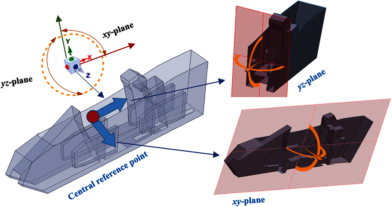
Figure 9: Two surface monitors parallel to the xy axis and the yz axis

It is well known that the flow characteristics of the fluid in a cockpit have effects on the pilot's general comfort, especially with various gravity effects. To obtain more additional details of the flow characteristic related to the basic flow mechanism in the cockpit, the velocity and turbulent kinetic energy are discussed in this section.
Fig. 10 illustrates the velocity distributions at the selected calibrated xy-plane and yz-plane for various inlet temperatures, inlet pressures, and gravitational acceleration conditions. For the flow information at the xy-plane (a-1, b-1, and c-1), it is found that the velocity distribution shows a strong inhomogeneous behavior at the forepart (inlet part) and the rear (outlet part), as well as a relatively homogeneous and stable feature at the middle of the cockpit, regardless of the applied initial conditions. Furthermore, it is found that the velocity gradient is highly consistent. This means that there is an insignificant change in the flow characteristics even as the parameter setting of the inlet temperature, pressure, and gravitational acceleration increases. This is mainly attributed to the small initial mass flux of 0.83 kg/h, which causes the numerical results to strongly prefer consistency.

Figure 10: Velocity profile in the selected xy-plane and yz-plane under different thermal conditions: a-1 and a-2 under inlet temperature of 283.15 K, inlet pressure of 0.5 MPa and gravitational acceleration of 1.0 g; b-1 and b-2 under inlet temperature of 288.15 K, inlet pressure of 1.0 MPa and gravitational acceleration of 1.5 g; c-1 and c-2 under inlet temperature of 293.15 K, inlet pressure of 1.5 MPa and gravitational acceleration of 2.0 g
Similar results are also captured at the yz-plane (a-2, b-2, and c-2) with the consistent velocity distribution, regardless of the types of increased inlet temperature, pressure, and gravitational acceleration that are applied. Interestingly, the extremum value of the local velocity appears on both sides of the figures. The velocity is often affected by the air inlet positions on both sides. The large velocity gradients near both narrowing regions are caused by the large recirculation velocity. When moving to the center, the induced maximum velocity magnitudes become smaller. The large slip of velocity gradient may be related to the variation. The profile of the temperature gradient can also be discussed using a three-dimensional flow transport equation, as shown in Section 2.3. The variable turbulent dissipation rate and the turbulent kinetic generation term induce an inhomogeneous velocity distribution. Overall, there is a strong inhomogeneous flow behavior and a great consistency in the velocity distribution, which is not changed by the applied combination conditions for either case.
In general, turbulent kinetic energy is regarded as a critical parameter to determine turbulent mixing ability. To better understand the distinct flow characteristics, a turbulent kinetic energy (TKE) analysis is carried out. As shown in Fig. 11, for xy-plane (a-1, b-1, and c-1), the core region of the TKE is located at the middle part, while the TKE can be negligible at the forepart and the rear region. Moreover, a large amount of inhomogeneous behavior is discovered at the middle part, which is also characterized at the yz-plane (a-2, b-2, and c-2). For the yz-plane, the large gradient region of the turbulent kinetic energy is close to both sides. Notably, the corresponding characteristics of the TKE are greatly similar to the velocity distribution.

Figure 11: Turbulent kinetic energy profile in the selected xy-plane and yz-plane under different thermal conditions: a-1 and a-2 under inlet temperature of 283.15 K, inlet pressure of 0.5 MPa and gravitational acceleration of 1.0 g; b-1 and b-2 under inlet temperature of 288.15 K, inlet pressure of 1.0 MPa and gravitational acceleration of 1.5 g; c-1 and c-2 under inlet temperature of 293.15 K, inlet pressure of 1.5 MPa and gravitational acceleration of 2.0 g
To some extent, a region with strong disturbance can be formed at the middle part. It is also found that there is an obvious consistency characteristic for the TKE distribution, irrespective of the initial setting of the thermal conditions. The air fluid almost fills the intermediate space, and the fluid velocity becomes small everywhere, resulting in low TKE. It is undeniable that a high TKE gradient will lead to a local fluid disturbance in the near-wall region. The development and decline of the TKE changes rapidly, which is beneficial for the local heat transfer.
3.2 Temperature Characteristics
The temperature distribution that is considered the important evaluation indicator of temperature homeostasis, is evaluated and analyzed. A temperature gradient is created by the temperature difference between the top and bottom walls.
As shown in Fig. 12, it is noticed that the large temperature gradient at the xy-plane and the yz-plane occurs at the top region where there is a radiant heat source. The heat transfers via turbulent flow from the top region. Hence, as shown in the xy-plane (a-1, b-1, and c-1), the high temperature fluid is mainly focused on the top region, and the low temperature fluid is located at the bottom region. The occurrence of the temperature difference is widespread in confined spaces. For the yz-plane (a-2, b-2, and c-2), the local extremum value of the airflow temperature occurs in the position that is characterized by the dramatic change of the TKE gradient. The temperature gradient is considered to be driven by the inhomogeneous temperature distribution. It is also revealed that the temperature distribution is more stable for various thermal conditions, and this demonstrates the great internal consistency of the temperature fields.

Figure 12: Temperature profile in the selected xy-plane and yz-plane under different thermal conditions: a-1 and a-2 under inlet temperature of 283.15 K, inlet pressure of 0.5 MPa and gravitational acceleration of 1.0 g; b-1 and b-2 under inlet temperature of 288.15 K, inlet pressure of 1.0 MPa and gravitational acceleration of 1.5 g; c-1 and c-2 under inlet temperature of 293.15 K, inlet pressure of 1.5 MPa and gravitational acceleration of 2.0 g
Next, the inhomogeneity coefficient of temperature is considered. The whole-field inhomogeneity coefficient (R) is defined as the ratio of the maximum difference to the average value at the same cross-section:
where the “Tmax” and “Tmin” represent the maximum and minimum values of fluid temperature, respectively, and “Tave” is the average temperature. Fig. 13 shows the results of temperature field inhomogeneity under different thermal conditions. The whole-field inhomogeneity coefficient (R) shows a decreasing trend as the inlet temperature, inlet pressure and gravitational acceleration increase. Clearly, the inlet temperature has the greatest effect on the R. This is because the inlet temperature gradually approaches the heat source temperature (295.15 K), and both cause the whole-field temperature to strongly prefer consistency and homogeneity. It should be noted that the R is insensitive to the changing pressure and gravitational acceleration. These two factors are insufficient to enhance the heat transfer effect in the heat source region, and the high and low temperature fluids remain inadequately mixed.

Figure 13: Evaluation of temperature field inhomogeneity under different thermal conditions: a-1 and a-2 under inlet temperature of 283.15 K, inlet pressure of 0.5 MPa and gravitational acceleration of 1.0 g; b-1 and b-2 under inlet temperature of 288.15 K, inlet pressure of 1.0 MPa and gravitational acceleration of 1.5 g; c-1 and c-2 under inlet temperature of 293.15 K, inlet pressure of 1.5 MPa and gravitational acceleration of 2.0 g
Overall, when implementing the space design of the cockpit, the internal flow and the temperature fields have to be taken into account. One of the well-validated critical evaluation factors concerns the determination of the steadiness of the field information. This means that the flow and temperature characteristics need to be constantly controlled in a reasonable and stable range, and thus satisfy the requirements of user experience and general comfort. Furthermore, the local flow and the temperature are dependent on many initial factors, i.e., the inlet temperature, inlet pressure, and gravitational acceleration. We have found that these factors have a very limited effect on the internal flow and temperature characteristics for a dedicated given initial mass flux of 0.83 kg/h. This result confirms that an optimized operating condition does exist and that this makes the flow and the temperature field more stable. From another perspective, it is also understood that the mass flux rather than the inlet temperature, inlet pressure, and gravitational acceleration has a great effect on the flow and temperature characteristics.
The complex structure in the cockpit, coupled with various operating conditions, can further exacerbate the inhomogeneous distributions. Consequently, it can be predicted that the internal fluid action caused by the interaction between the temperature field and the flow field will be very violent. Here, the analysis of the local temperature gradient at yz-plane that is induced by the temperature difference is further carried out under different initial conditions.
The results of the temperature-related gradient for the yz-plane are presented in Fig. 14. There is an evidently inhomogeneous disturbance behavior along the y axis that is mainly caused by temperature difference between the top and bottom walls. Typically, this inhomogeneity found along the y axis is predominantly related to the temperature distribution. The key feature of the temperature gradient trend is the ability to be less sensitive to the various inlet temperatures, inlet pressures, and gravitational accelerations. Specifically, a common distribution feature of the temperature gradient can be divided into two types: 1) slight changes of the gradient between 0 and 1.0 m on the y axis; and 2) dramatic changes of the gradient between 1.25 and 1.5 m on the y axis. The high temperature in the top region is responsible for this gradient structure, which cannot even be regulated by the given operating conditions. In other words, it is critical to conduct the structure design of the cockpit in conditions such that the heat source in the top region is a non-ignorable factor. Moreover, the impact of forced convection with thermal radiation is a relevant field in which further studies are required.

Figure 14: Temperature gradient distribution on the yz-plane along y axis under different thermal conditions: (a) under inlet temperature of 278.15, 283.15, 288.15 and 293.15 K; (b) under gravitational acceleration of 1.0, 1.5 and 2.0 g; (c) under inlet pressure of 0.5, 1.0, 1.5 and 2.0 MPa
The internal flow and temperature fields are studied with a high-accuracy SST k-ω turbulence model to improve comfort in a cockpit. The flow and temperature characteristics are numerically evaluated and analyzed for various initial inlet temperatures, inlet pressures, and gravitational accelerations. Additionally, the common characteristics and mechanisms of the inhomogeneous distribution are described in detail. The main conclusions are summarized as follows:
1) To accurately predict the inhomogeneous behaviors, the proposed RANS turbulence models are necessarily evaluated, and it is found that SST k-w (2 eqn) has a better predictive performance for the modeling of the inhomogeneous behaviors.
2) The flow and temperature fields show a distinct inhomogeneous distribution at the fixed xy-plane and the yz-plane. The results indicate that the flow field shows a stable state at the middle part of the cockpit, and the temperature field has a large gradient that focuses on the top region.
3) The results indicate that the flow and temperature distribution are stable, and that they cannot be regulated by various operating conditions. Moreover, the mass flux and the heat source have a critical impact on the inhomogeneous distribution of the flow and temperature fields.
4) Two typical gradient features of temperature are discovered. The near-wall region shows a dramatic disturbance, while the temperature-related gradient is relatively smooth near the bottom region of the cockpit. This study, therefore, has important implications for cockpit design.
Funding Statement: This work was sponsored by the Fundamental Research Funds for the Central Universities. (Project No. 31020190504004).
Conflicts of Interest: The authors declare that they have no conflicts of interest to report regarding the present study.
1. Salmi, M., Menni, Y., Chamkha, A. J., Ameur, H., Maouedj, R. et al. (2021). CFD-Based simulation and analysis of hydrothermal aspects in solar channel heat exchangers with various designed vortex generators. Computer Modeling in Engineering & Sciences, 126(1), 147–173. DOI 10.32604/cmes.2021.012839. [Google Scholar] [CrossRef]
2. Liu, M., Liu, J., Ren, J., Liu, L., Chen, R. et al. (2020). Bacterial community in commercial airliner cabins in China. International Journal of Environmental Health Research, 30(3), 284–295. DOI 10.1080/09603123.2019.1593329. [Google Scholar] [CrossRef]
3. Tang, Z., Cui, X., Guo, Y., Jiang, N., Dai, S. et al. (2017). Near fields of gasper jet flows with wedged nozzle in aircraft cabin environment. Building and Environment, 125(15), 99–110. DOI 10.1016/j.buildenv.2017.08.047. [Google Scholar] [CrossRef]
4. Gupta, P., Rajput, S. P. S. (2015). Optimised cockpit heat load analysis using skin temperature predicted by CFD and validation by thermal mapping to improve the performance of fighter aircraft. Defence Science Journal, 65(1), 12–24. DOI 10.14429/dsj.65.7200. [Google Scholar] [CrossRef]
5. Zhang, Y., Liu, J., Pei, J., Li, J., Wang, C. (2017). Performance evaluation of different air distribution systems in an aircraft cabin mockup. Aerospace Science and Technology, 70, 359–366. DOI 10.1016/j.ast.2017.08.009. [Google Scholar] [CrossRef]
6. Bravo-Mosquera, P. D., Abdalla, A. M., Ceron-Munoz, H. D., Catalano, F. M. (2019). Integration assessment of conceptual design and intake aerodynamics of a non-conventional air-to-ground fighter aircraft. Aerospace Science and Technology, 86, 497–519. DOI 10.1016/j.ast.2019.01.059. [Google Scholar] [CrossRef]
7. Cahill, J., McDonald, N., Morrison, R., Lynch, D. (2016). The operational validation of new cockpit technologies supporting all conditions operations. a case study. Cognition, Technology & Work, 18(3), 479–509. DOI 10.1007/s10111-016-0380-4. [Google Scholar] [CrossRef]
8. Nagda, N. L., Hodgson, M. (2010). Low relative humidity and aircraft cabin air quality. Indoor Air, 11(3), 200–214. DOI 10.1034/j.1600-0668.2001.011003200.x. [Google Scholar] [CrossRef]
9. Li, J., Liu, J., Wang, C., Jiang, N., Cao, X. (2016). PIV methods for quantifying human thermal plumes in a cabin environment without ventilation. Journal of Visualization, 20(3), 535–548. DOI 10.1007/s12650-016-0404-4. [Google Scholar] [CrossRef]
10. Gupta, P., Rajput, S. P. S. (2015). Computational fluid dynamics and thermal analysis to estimate the skin temperature of cockpit surface in various flight profiles. Journal of Aerospace Engineering, 28(1), 04014056. DOI 10.1061/(ASCE)AS.1943-5525.0000345. [Google Scholar] [CrossRef]
11. Wu, T. Y., Jiang, Y. Z., Su, Y. Z., Yeh, W. C. (2020). Using simplified swarm optimization on multiloop fuzzy PID controller tuning design for flow and temperature control system. Applied Sciences, 10(23), 8472. DOI 10.3390/app10238472. [Google Scholar] [CrossRef]
12. Wang, C., Li, J., Li, J., Guo, Y., Jiang, N. (2017). Turbulence characterization of instantaneous airflow in an aisle of an aircraft cabin mockup. Build Environ, 116(1), 207-217. DOI 10.1016/j.buildenv.2017.02.015. [Google Scholar] [CrossRef]
13. Liu, W., Wen, J., Chao, J., Yin, W., Shen, C. et al. (2012). Accurate and high-resolution boundary conditions and flow fields in the first-class cabin of an MD-82 commercial airliner. Atmospheric Environment, 56, 33–44. DOI 10.1016/j.atmosenv.2012.03.039. [Google Scholar] [CrossRef]
14. Bosbach, J., Pennecot, J., Wagner, C., Raffel, M., Lerche, T. et al. (2006). Experimental and numerical simulations of turbulent ventilation in aircraft cabins. Energy, 31, 694–705, DOI 10.1016/j.energy.2005.04.015. [Google Scholar] [CrossRef]
15. Pang, L. P., Luo, K., Yuan, Y. P., Mao, X. D., Fang, Y. F. (2020). Thermal performance of helicopter air conditioning system with lube oil source (LOS) heat pump. Energy, 190, 116446. DOI 10.1016/j.energy.2019.116446. [Google Scholar] [CrossRef]
16. Fan, J. L., Zhou, Q. Y. (2019). A review about thermal comfort in aircraft. Journal of Thermal Science, 28(2), 169–183. DOI 10.1007/s11630-018-1073-5. [Google Scholar] [CrossRef]
17. Zhang, Z., Chen, X., Mazumdar, S., Zhang, T., Chen, Q. (2009). Experimental and numerical investigation of airflow and contaminant transport in an airliner cabin mockup. Building and Environment, 44(1), 85–94. DOI 10.1016/j.buildenv.2008.01.012. [Google Scholar] [CrossRef]
18. Li, B., Duan, R., Li, J. (2016). Experimental studies of thermal environment and contaminant transport in a commercial aircraft cabin with gaspers on. Indoor Air, 26, 806-819. DOI 10.1111/ina.12265. [Google Scholar] [CrossRef]
19. Danca, P., Bode, F., Nastase, I., Meslem, A. (2018). CFD simulation of a cabin thermal environment with and without human body–thermal comfort evaluation. E3S Web of Conferences, vol. 32, 01018. [Google Scholar]
20. Yao, Z., Zhang, X., Yang, C., He, F. (2015). Flow characteristics and turbulence simulation for an aircraft cabin environment. Procedia Engineering, 121, 1266–1273. DOI 10.1016/j.proeng.2015.09.156. [Google Scholar] [CrossRef]
21. You, R., Chen, J., Shi, Z., Liu, W., Lin, C. H. et al. (2016). Experimental and numerical study of airflow distribution in an aircraft cabin mock-up with a gasper on. Journal of Building Performance Simulation, 9(5), 555–566. DOI 10.1080/19401493.2015.1126762. [Google Scholar] [CrossRef]
22. Lin, C., Horstman, R., Ahlers, M., Sedgwick, L., Dunn, K. et al. (2005). Numerical simulation of airflow and airborne pathogen transport in aircraft cabins–Part 1. Numerical simulation of the flow field. ASHRAE Transactions, 111(1), 755–763. [Google Scholar]
23. Lin, C., Horstman, R., Ahlers, M., Sedgwick, L., Dunn, K. et al. (2005). Numerical simulation of airflow and airborne pathogen transport in aircraft cabins–Part 2. Numerical simulation airborne pathogen transport. ASHRAE Transactions, 111, 764–768. [Google Scholar]
24. Afshari, F., Sahin, B., Khanlari, A., Manay, E. (2020). Experimental optimization and investigation of compressor cooling fan in an air-to-water heat pump. Heat Transfer Research, 51(4), 319–331. DOI 10.1615/HeatTransRes.2019030709. [Google Scholar] [CrossRef]
25. Yang, C., Zhang, X., Yao, Z., Cao, X., Liu, J. et al. (2016). Numerical study of the instantaneous flow fields by large eddy simulation and stability analysis in a single aisle cabin model. Building and Environment, 96, 1–11. DOI 10.1016/j.buildenv.2015.10.022. [Google Scholar] [CrossRef]
26. Isukapalli, S. S., Mazumdar, S., George, P., Wei, B., Jones, B. et al. (2013). Computational fluid dynamics modeling of transport and deposition of pesticides in an aircraft cabin. Atmospheric Environment, 68, 198–207. DOI 10.1016/j.atmosenv.2012.11.019. [Google Scholar] [CrossRef]
27. Baker, A., Ericson, S., Orzechowski, J., Wong, K., Garner, R. (2006). Aircraft passenger cabin ECS-generated ventilation velocity and mass transport CFD simulation. velocity field validation. Journal of the IEST, 49(2), 51–83. DOI 10.17764/jiet.49.2.j15866q30r09r4m1. [Google Scholar] [CrossRef]
28. Li, F., Lee, E. S., Liu, J., Zhu, Y. (2015). Predicting self-pollution inside school buses using a CFD and multi-zone coupled model. Atmospheric Environment, 107, 16–23, DOI 10.1016/j.atmosenv.2015.02.024. [Google Scholar] [CrossRef]
29. Qian, H., Li, Y., Nielsen, P., Huang, X. (2009). Spatial distribution of infection risk of SARS transmission in a hospital ward. Building and Environment, 44(8), 1651–1658. DOI 10.1016/j.buildenv.2008.11.002. [Google Scholar] [CrossRef]
30. Zhang, T., Chen, Q. Y. (2007). Novel air distribution systems for commercial aircraft cabins. Building and Environment, 42(4), 1675–1684. DOI 10.1016/j.buildenv.2006.02.014. [Google Scholar] [CrossRef]
31. Du, X. Y. (2017). Air supply parameters optimization of personal nozzle system and evaluation on thermal environment in aircraft cabins (Ph.D Thesis). Chongqing University. [Google Scholar]
32. Wang, W. Y. (2015). Key technologies of aircraft cockpit's ergonomic design and comprehensive evaluation (Ph.D Thesis). Northwestern Polytechnical University. [Google Scholar]
33. Tian, Y. S., Karyiannis, T. G. (2000). Low turbulence natural convection in an air filled square cavity. Part 1. The thermal and fluid flow fields. Journal of Heat and Mass Transfer, 43(6), 849–866. DOI 10.1016/S0017-9310(99)00199-4. [Google Scholar] [CrossRef]
 | This work is licensed under a Creative Commons Attribution 4.0 International License, which permits unrestricted use, distribution, and reproduction in any medium, provided the original work is properly cited. |