| Computer Modeling in Engineering & Sciences |
DOI: 10.32604/cmes.2022.018492
ARTICLE
Transferable Features from 1D-Convolutional Network for Industrial Malware Classification
1School of Computer and Communication Engineering, University of Science and Technology Beijing, Beijing, 100083, China
2Beijing Key Laboratory of Knowledge Engineering for Materials Science, Beijing, 100083, China
3Shunde Graduate School, University of Science and Technology Beijing, Foshan, 528399, China
4Beijing Intelligent Logistics System Collaborative Innovation Center, Beijing, 101149, China
*Corresponding Author: Xiong Luo. Email: xluo@ustb.edu.cn
Received: 28 July 2021; Accepted: 28 September 2021
Abstract: With the development of information technology, malware threats to the industrial system have become an emergent issue, since various industrial infrastructures have been deeply integrated into our modern works and lives. To identify and classify new malware variants, different types of deep learning models have been widely explored recently. Generally, sufficient data is usually required to achieve a well-trained deep learning classifier with satisfactory generalization ability. However, in current practical applications, an ample supply of data is absent in most specific industrial malware detection scenarios. Transfer learning as an effective approach can be used to alleviate the influence of the small sample size problem. In addition, it can also reuse the knowledge from pre-trained models, which is beneficial to the real-time requirement in industrial malware detection. In this paper, we investigate the transferable features learned by a 1D-convolutional network and evaluate our proposed methods on 6 transfer learning tasks. The experiment results show that 1D-convolutional architecture is effective to learn transferable features for malware classification, and indicate that transferring the first 2 layers of our proposed 1D-convolutional network is the most efficient way to reuse the learned features.
Keywords: Transfer learning; malware classification; sequence data modeling; convolutional network
In the era of digitalization and intelligence, an increasing number of industrial devices are connected to the Internet and the generated data can be collected and analyzed more efficiently for personalized service and industrial production. Meanwhile, those devices suffer from various cyber-attacks [1]. Malicious attackers can spread malware, such as viruses, Trojan horses, or ransomware, to compromise industrial systems. To avoid the damages from the malware, an extensive exploration about deep neural networks, recurrent neural network (RNN), and convolutional neural network (CNN) for the industrial Internet of Things (IoT) and cyber-physical system security suggests that deep learning is a powerful tool to detect and classify malware [2 –6].
Towards the deep learning solutions for the malware detection and classification tasks, the general idea is to train a deep learning model from scratch following the classical supervised training paradigm. However, the small sample size problem in practical applications degrades the performance severely in deep learning. Due to different kinds of heterogeneous devices in industrial systems and the specificity of malware, the small sample size problem often arises when applying deep learning techniques. Following that, transfer learning is a sophisticated paradigm to alleviate such an issue. In recent researches, transfer learning is widely applied to image-based malware analysis [7–10]. The general procedures in such a scenario include: 1) converting every malware instance into a gray-scale or RGB image; 2) pre-training a CNN on a large source dataset, e.g., a ResNet-50 based on ImageNet; 3) transferring the convolutional layers in the pre-trained CNN to a new randomly initialized network, freezing the parameters in the convolutional layers, and fine-tuning the parameters in the fully connected layers on target dataset. Here, the key assumption is that the learned color blobs and Gabor filters from the CNN are also applicable to identify the texture of malware images. It is noted that the differences between natural images and malware images are obvious, which means a semantic gap exists.
To overcome issue of the semantic gap, we select opcode and application programming interface (API) sequence for malware behavior representation. Here, the functionality of various programs in different platforms is a process of executing commands sequentially, which means the opcode or API sequence is a more general and precise behavior representation for malware than image-based representation. Among the data-driven malicious sequence modeling architectures, RNN is a common network structure for modeling sequence data due to its weights sharing mechanism on the time dimension. In the era of big data, processing massive amounts of data has become the norm, and parallel computing is now an essential method to handle it. However, RNN is unable to gain benefit from the graphics processing unit (GPU) with parallel computing ability because of its sequential computation process. Hence, in order to make full use of the parallel computing ability of GPU, a new 1D-convolutional-based sequence data modeling scheme was developed and its excellent performance was validated in language modeling [11,12] and time-series classification subsequently [13]. Based on the discussions above, a transfer learning-enhanced 1D-convolutional network architecture is explored for the specific sequence modeling task in this paper, i.e., malware sequence classification. The contributions of this paper are summarized as follows:
• We propose a 1D-convolutional architecture to perform transfer learning and evaluate 3 convolutional strategies on 6 transfer learning tasks. The experiment results show that the 1D-convolutional network can effectively learn transferable features for malware classification.
• We conduct several experiments to identify the practical way to transfer the parameters of convolutional layer. Moreover, the experiment results show that transfer learning is an effective approach to reduce the training time.
The remainder of this paper is organized as follows. Section 2 overviews some recent works on sequence data modeling. The proposed network architecture is described in Section 3. Our experimental results are presented in Section 4. The conclusion of this paper is stated in Section 5.
Deep learning and transfer learning are widely explored in sequence data modeling. In this section, for sequence data modeling task, the developed deep learning models, especially the 1D-convolutional networks on malicious sequence data, are overviewed firstly. Then, the transfer learning models on sequence data are analyzed.
2.1 Deep Learning for Sequence Data Modeling
For malware classification, opcode and API sequences are usually used for malware behavior representation. HaddadPajouh et al. [14] adopted long short-term memory (LSTM) for ARM-based IoT malware detection based on opcode sequence. Kang et al. [15] and Jha et al. [16] used LSTM to classify different malware families based on API sequence and opcode. To benefit from the parallel computing ability of GPU, the 1D-convolutional network is proposed for sequence data modeling. Shelhamer et al. [17] proposed a fully convolutional network (FCN) architecture for semantic segmentation. Wang et al. [13] modified the original FCN with one-dimensional kernels and replaced the last layer of FCN with fully connected layers and a softmax layer for time series classification. After that, some researchers explored the potential of 1D-convolutional networks for malware detection. Hasegawa et al. [18] used a 1D-convolutional network to detect Android malware. Then, to prevent information leakage from the future into the past, a specific temporal convolutional network (TCN) [19] was utilized to categorize malware into different families in the field of IoT malware classification [20].
2.2 Transfer Learning for Sequence Data Modeling
The major assumption from the classical supervised learning scheme is that training and future data follow the same distribution. However, this assumption fails in some industrial malware detection cases, since malicious training instances from heterogeneous devices may not satisfy the same feature distribution. In addition, the training dataset may easily get out of date in the era of big data [21]. Hence, knowledge transfer will be a useful technique to improve the performance of deep learning models. Fawaz et al. [22] extensively explored the transferable ability of 1D-FCN for time series classification, and their experiment results showed that knowledge transfer is beneficial to performance enhancement. Subsequently, Gao et al. [23] explored a semi-supervised transfer learning technique to alleviate the influence of the small sample size problem.
Meanwhile, there are also some problems in the use of transfer learning. They can be summarized as follows: 1) what to transfer? 2) where to transfer? and 3) how to transfer? Currently, the mainstream transfer learning paradigm is based on pre-training and fine-tuning strategies, as illustrated in Fig. 1, including 1) pre-training a deep learning model on source domain; 2) transferring the learned weights of the first few layers (i.e., what to transfer); 3) freezing the weights of transferred layers and retraining the parameters of the rest on target domain (i.e., how to transfer). In this paper, we follow the general strategy mentioned above, and determine where to transfer the layers pre-trained on the source domain in accordance with the experiment strategy developed in [24].

Figure 1: The general transfer learning paradigm using pre-training and fine-tuning strategies
In this section, we give a formal definition of the transfer learning task and descriptions of data preprocessing steps firstly. Then, the proposed 1D-convolutional network architecture is introduced.
Here, the schematic diagram of our proposed method is illustrated in Fig. 2.

Figure 2: The schematic diagram of our proposed method
Domain and task are basic conceptions in transfer learning. A domain D is defined as
Based on the definition above, the transfer learning can be defined as: given a source supervised learning task < Ds, Ts > and a target supervised learning task < Dt, Tt > , the transfer learning utilizes the knowledge learned on the source task to improve the performance of discriminant function on the target task. Since opcode and API in different datasets used in this paper are not consistent, which means
To ensure the feature space of different datasets has the same mathematic representation, we utilize the GloVe word embedding algorithm [25] to align the feature space. Here, we treat each API or opcode as a word. The procedure of data preprocessing is illustrated in Fig. 3. The extraction of opcode and API can be implemented through the use of reverse engineering tools or the monitor for the dynamic execution process of malware in a sandbox.

Figure 3: The procedure of data preprocessing
GloVe is a word embedding algorithm that takes advantage of both global statistical information and local context. Before training the word vectors, we need to use a sliding window to compute the word-word co-occurrence matrix
Here,
After the convergence of the training process,
In this paper, we redesign the 1D-FCN architecture proposed in [13]. To stabilize the training process, we replace the batch normalization with layer normalization and add shortcut connections to 1D-FCN, which is illustrated in Fig. 4. In this figure, ‘ReLU’ means the rectified liner unit (ReLU) activation function widely used in neural networks, and it will set negative output to zero and keep non-negative output unchanged. Meanwhile, for multiclass classification task, ‘Softmax’ is an activation widely used as the last layer to output possibility distribution.
The functionality of basic 1D-convolutional operation is shown in Fig. 5a, and the illustration of 1D-convolution with dilation is shown in Fig. 5b. In Fig. 5, each blue column represents a word vector obtained from GloVe word embedding algorithm, and green columns denote the 1D-kernel. A 1D-kernel acts like a sliding window and travels from left to right to perform convolutional operation. Compared to conventional 1D-kernel, 1D-kernel with dilation can compute larger receptive field, as shown in Fig. 5b. To prevent information leakage from the future into the past, padding zeros with L −1 length will be applied before convolution. Here, L denotes the length of 1D-kernel, and such operations are called causal convolution.

Figure 4: The architecture of our proposed 1D-convolutional network

Figure 5: Illustration of 1D-convolution. (a) 1D-Conv without dilation (b) 1D-Conv with dilation
With the architecture we proposed, we evaluate 3 different convolutional strategies: 1) FCN [13] (conventional 1D-convolution as shown in Fig. 5a; 2) TCN [19] (1D-convolution with dilation as shown in Fig. 5b, where the dilation is not a constant but expansion with the exponential rate, i.e., the dilation factors of the convolutional layers are
Since different convolutional strategies share the same network architecture in our experiment settings, we select the gated convolutional layer (GCL) as our baseline convolutional strategy to tune the hyper-parameters. The GCL can be expressed by (3):
where X is the input sequence data, K and M are two different 1D-convolutional kernels with the same shape, ‘ * ’ is the convolution operator, and ‘
Shortcut Connection During the training process of a deep learning model, to solve the gradient vanishing problem, the shortcut connection was proposed in [26]. It is effective and concise shown in (4):
where
Layer Normalization Compared with batch normalization, the layer normalization (LN) is helpful to stabilize the training process, and it is more suitable for sequence data and independent of batch size [27], since its computation is limited to one single instance. The computation of LN is defined in (5):
where
Positional Encoding To enrich the input sequence representation, positional encoding, which can provide the current positional information for the 1D convolution, is introduced in the proposed model. The utilized positional encoding can be formalized by (6) [28]:
where q denotes the q-position in the sequence, d is the positional embedding size, k denotes the k-th entry of the positional vector. In addition, its visualization is illustrated in Fig. 6. Each row in Fig. 6 represents a position vector, and as time step increases, the changes in the high-dimensional component of the position vector become more significant. In this paper, the addition operation between the GloVe vector and positional vector is applied before the 1D-convolutional network.
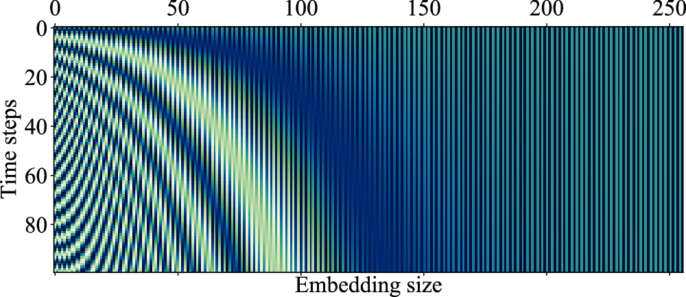
Figure 6: Visualization of positional encoding
4 Experimental Results and Discussion
In our experiments, we choose Python 3.8, PyTorch 1.7 and CUDA 11.0 to build the convolutional network architecture. The proposed model is tested in a computer that runs Ubuntu and consists of NVIDIA 1080Ti, Intel(R) Xeon(R) CPU E5-2673 v3 and 64 GB memory.
There are two Windows platform datasets, including a bigger one, i.e., the Microsoft Malware Classification Challenge (BIG 2015) dataset from Kaggle competition [29], and a smaller one, i.e., the Windows portable executable (PE) dataset from Allan et al. [30]. To make full use of the diversity of the samples and the different malware families in the original datasets, we construct different transfer learning tasks to evaluate our proposed models more comprehensively. Hence, these two datasets are reorganized to conduct the experiments. After the data reorganization, the former bigger dataset is comprised of sequential opcode and API function names, and the latter one is comprised of API sequences. To extensively explore the performance of our proposed architecture, the former Kaggle dataset is split into 3 sub-datasets

Here, GloVe word embedding algorithm is applied before the training process of the proposed architecture, and the hyper-parameters for the GloVe algorithm are listed in Table 2. Towards the proposed architecture, the key hyper-parameters, including output channels, kernel size in the convolutional layers, and the hidden dimension in the fully connected layer are determined by cross-validation. In addition, other hyper-parameters listed in Table 3 are selected by our engineering experience motivated by [13 –15].


The cross-validation results, i.e., accuracy (mean

Figure 7: Cross-validation results (mean
To evaluate the performance of our proposed 1D-convolutional architecture comprehensively, GCN, TCN and FCN are selected as comparative algorithms due to their validated excellent performance in many other tasks [11,19,22]. To identify where to transfer the learned weights of the 1D-convolution network, we evaluate GCN on 4 transfer learning tasks:

Figure 8: Accuracy with different transferred layers. (a) AnX tasks using GCN. (b) AnX tasks using TCN. (c) AnX tasks using FCN. (d) BnX tasks using GCN. (e) BnX tasks using TCN. (f)BnX tasks using FCN

Figure 9: Ratio with different transferred layers. (a) GCN. (b) TCN. (c) FCN
We evaluate 3 different 1D-convolutional strategies on 6 transfer learning tasks, as shown in Table 4. Here, ‘XCN-n’ means transferring the first n layers of XCN, and each row in Table 4 demonstrates experimental results of XCN-n on different transfer tasks. For a fair comparison, TCN and FCN have the same hyper-parameters as GCN. From Table 4, in most cases, transferring the first 2 convolutional layers is better than transferring the first 3 layers directly, since the top convolutional layer is more task-specific than previous layers. However, the improvement is slight or even negative when the number of training instances in the target domain is small (i.e., D and E).

The other conclusion revealed by Table 4 is that the source domain, which contains more behavior representation, is more capable of improving the performance of transfer learning tasks. For example, the source domain A contains 1070 opcodes (APIs) and B contains 680 opcodes (APIs). Hence, the performance of
In this paper, we propose a 1D-convolutional architecture for malware classification, and then evaluate the architecture via 3 convolutional strategies on 6 transfer learning tasks. Our experimental results verify that the transfer learning technique is an effective approach to reuse the learned knowledge from other datasets, and transferring the first 2 convolutional layers is a better choice for this malware classification task. Moreover, the experimental results also demonstrate the time reduction in the training process. For future work, our proposed method is expected to be evaluated on other extensive tasks, and domain adaption techniques will be further investigated for performance improvement.
Funding Statement: This work was supported in part by the National Natural Science Foundation of China under Grants U1836106 and 81961138010, in part by the Beijing Natural Science Foundation under Grants 19L2029 and M21032, in part by the Scientific and Technological Innovation Foundation of Foshan under Grants BK20BF010 and BK21BF001, in part by the Scientific and Technological Innovation Foundation of Shunde Graduate School, USTB, under Grant BK19BF006, and in part by the Fundamental Research Funds for the University of Science and Technology Beijing under Grant FRF-BD-19-012A.
Conflicts of Interest: The authors declare that they have no conflicts of interest to report regarding the present study.
1. Lee, J., Kim, J., Seo, J. (2019). Cyber attack scenarios on smart city and their ripple effects. Proceedings of the International Conference on Platform Technology and Service, pp. 1–5. Jeju, Korea, IEEE. [Google Scholar]
2. Al-Garadi, M. A., Mohamed, A., Al-Ali, A. K., Du, X. J., Ali, I. et al. (2020). A survey of machine and deep learning methods for Internet of Things (IoT) security. IEEE Communications Surveys & Tutorials, 22(3), 1646–1685. DOI 10.1109/COMST.2020.2988293. [Google Scholar] [CrossRef]
3. Ma, H., Tian, J., Qiu, K., Lo, D., Gao, D. et al. (2021). Deep-learning-based app sensitive behavior surveillance for android powered cyber-physical systems. IEEE Transactions on Industrial Informatics, 17(8), 5840–5850. DOI 10.1109/TII.2020.3038745. [Google Scholar] [CrossRef]
4. Chen, M., Li, Y., Luo, X., Wang, W., Wang, L. et al. (2019). A novel human activity recognition scheme for smart health using multilayer extreme learning machine. IEEE Internet of Things Journal, 6(2), 1410–1418. DOI 10.1109/JIOT.2018.2856241. [Google Scholar] [CrossRef]
5. Luo, X., Sun, J., Wang, L., Wang, W., Zhao, W. et al. (2018). Short-term wind speed forecasting via stacked extreme learning machine with generalized correntropy. IEEE Transactions on Industrial Informatics, 14(11), 4963–4971. DOI 10.1109/TII.2018.2854549. [Google Scholar] [CrossRef]
6. Luo, X., Li, J., Chen, M., Yang, X., Li, X. (2021). Ophthalmic disease detection via deep learning with a novel mixture loss function. IEEE Journal of Biomedical and Health Informatics, 25(9), 3332–3339. DOI 10.1109/JBHI.2021.3083605. [Google Scholar] [CrossRef]
7. Rezende, E., Ruppert, G., Carvalho, T., Ramos, F., de Geus, P. (2017). Malicious software classification using transfer learning of resNet-50 deep neural network. Proceedings of the 16th IEEE International Conference on Machine Learning and Applications, pp. 1011–1014. Cancun, Mexico, IEEE. [Google Scholar]
8. Bhodia, N., Prajapati, P., Di Troia, F., Stamp, M. (2019). Transfer learning for image-based malware classification. Proceedings of the 5th International Conference on Information Systems Security and Privacy, pp. 719–726. Prague, Czech Republic, SciTePress. [Google Scholar]
9. Nahmias, D., Cohen, A., Nissim, N., Elovici, Y. (2020). Deep feature transfer learning for trusted and automated malware signature generation in private cloud environments. Neural Networks, 124, 243–257. DOI 10.1016/j.neunet.2020.01.003. [Google Scholar] [CrossRef]
10. Sudhakar, Kumar, S. (2021). MCFT-CNN: Malware classification with fine-tune convolution neural networks using traditional and transfer learning in internet of things. Future Generation Computer Systems, 125, 334–351. DOI 10.1016/j.future.2021.06.029. [Google Scholar] [CrossRef]
11. Dauphin, Y. N., Fan, A., Auli, M., Grangier, D. (2017). Language modeling with gated convolutional networks. Proceedings of the 34th International Conference on Machine Learning, pp. 933–941. Sydney, Australia, IMLS. [Google Scholar]
12. Gehring, J., Auli, M., Grangier, D., Yarats, D., Dauphin, Y. N. (2017). Convolutional sequence to sequence learning. Proceedings of the 34th International Conference on Machine Learning, pp. 2029–2042. Sydney, Australia, IMLS. [Google Scholar]
13. Wang, Z., Yan, W., Oates, T. (2017). Time series classification from scratch with deep neural networks: A strong baseline. Proceedings of the International Joint Conference on Neural Networks, pp. 1578–1585. Anchorage, AK, USA, IEEE. [Google Scholar]
14. HaddadPajouh, H., Dehghantanha, A., Khayami, R., Choo, K. K. R. (2018). A deep recurrent neural network based approach for internet of things malware threat hunting. Future Generation Computer Systems, 85, 88–96. DOI 10.1016/j.future.2018.03.007. [Google Scholar] [CrossRef]
15. Kang, J., Jang, S., Li, S., Jeong, Y. S., Sung, Y. (2019). Long short-term memory-based malware classification method for information security. Computers & Electrical Engineering, 77, 366–375. DOI 10.1016/j.compeleceng.2019.06.014. [Google Scholar] [CrossRef]
16. Jha, S., Prashar, D., Long, H. V., Taniar, D. (2020). Recurrent neural network for detecting malware. Computers & Security, 99, 102037. DOI 10.1016/j.cose.2020.102037. [Google Scholar] [CrossRef]
17. Shelhamer, E., Long, J., Darrell, T. (2017). Fully convolutional networks for semantic segmentation. IEEE Transactions on Pattern Analysis and Machine Intelligence, 39(4), 640–651. DOI 10.1109/TPAMI.2016.2572683. [Google Scholar] [CrossRef]
18. Hasegawa, C., Iyatomi, H. (2018). One-dimensional convolutional neural networks for android malware detection. Proceedings of the IEEE 14th International Colloquium on Signal Processing & Its Applications, pp. 99–102. Penang, Malaysia, IEEE. [Google Scholar]
19. Bai, S., Kolter, J. Z., Koltun, V. (2018). An empirical evaluation of generic convolutional and recurrent networks for sequence modeling. arXiv:1803.01271. [Google Scholar]
20. Sun, J., Luo, X., Gao, H., Wang, W., Gao, Y. et al. (2020). Categorizing malware via a word2vec-based temporal convolutional network scheme. Journal of Cloud Computing, 9(1), 53. DOI 10.1186/s13677-020-00200-y. [Google Scholar] [CrossRef]
21. Pan, S. J., Yang, Q. (2010). A survey on transfer learning. IEEE Transactions on Knowledge and Data Engineering, 22(10), 1345–1359. DOI 10.1109/TKDE.2009.191. [Google Scholar] [CrossRef]
22. Fawaz, H. I., Forestier, G., Weber, J., Idoumghar, L., Muller, P. A. (2018). Transfer learning for time series classification. Proceedings of the IEEE International Conference on Big Data, pp. 1367–1376. Seattle, WA, USA, IEEE. [Google Scholar]
23. Gao, X., Hu, C., Shan, C., Liu, B., Niu, Z. et al. (2020). Malware classification for the cloud via semi-supervised transfer learning. Journal of Information Security and Applications, 55, 102661. DOI 10.1016/j.jisa.2020.102661. [Google Scholar] [CrossRef]
24. Yosinski, J., Clune, J., Bengio, Y., Lipson, H. (2014). How transferable are features in deep neural networks? Proceedings of the 27th International Conference on Neural Information Processing Systems, pp. 3320–3328. Montreal, QC, Canada, NIPSF. [Google Scholar]
25. Pennington, J., Socher, R., Manning, C. (2014). Glove: Global vectors for word representation. Proceedings of the Conference on Empirical Methods in Natural Language Processing, pp. 1532–1543. Doha, Qatar, ACL. [Google Scholar]
26. He, K., Zhang, X., Ren, S., Sun, J. (2016). Deep residual learning for image recognition. Proceedings of the IEEE Conference on Computer Vision and Pattern Recognition, pp. 770–778. Las Vegas, NV, USA, IEEE. [Google Scholar]
27. Ba, J. L., Kiros, J. R., Hinton, G. E. (2016). Layer normalization. arXiv:1607.06450. [Google Scholar]
28. Vaswani, A., Shazeer, N., Parmar, N., Uszkoreit, J., Jones, L. et al. (2017). Attention is all you need. Proceedings of the 31st International Conference on Neural Information Processing Systems, pp. 5999–6009. Long Beach, CA, USA, NIPSF. [Google Scholar]
29. Ronen, R., Radu, M., Feuerstein, C., Yom-Tov, E., Ahmadi, M. (2018). Microsoft malware classification challenge. arXiv:1802.10135. [Google Scholar]
30. Allan, N., Ngubiri, J. (2019). Windows PE API calls for malicious and benigin programs. DOI 10.13140/RG.2.2.14417.68960. [Google Scholar] [CrossRef]
 | This work is licensed under a Creative Commons Attribution 4.0 International License, which permits unrestricted use, distribution, and reproduction in any medium, provided the original work is properly cited. |