Computer Modeling in Engineering & Sciences

DOI: 10.32604/cmes.2022.017729

ARTICLE

A Mathematical Model and Simulations of Low Temperature Nitriding

Bogusław Bożek1, Lucjan Sapa1,*, Katarzyna Tkacz-Śmiech2, Marek Danielewski2 and Janusz Rybak2

1AGH University of Science and Technology, Faculty of Applied Mathematics, Cracow, 30-059, Poland
2AGH University of Science and Technology, Faculty of Materials Science and Ceramics, Cracow, 30-059, Poland
*Corresponding Author: Lucjan Sapa. Email: sapa@agh.edu.pl
Received: 02 June 2021; Accepted: 10 September 2021

List of symbols

1  Introduction

Nitriding is a thermochemical surface treatment carried out below eutectoid temperature. In the method, a surface of a solid substrate is modified by inserting (diffusion) of nitrogen from the gas atmosphere, which leads to the development of a compound layer and diffusion zone near the substrate surface [1–3]. Nitriding has shown the potential to enhance mechanical properties of the surface layer. The compound layer can improve wear and corrosion resistance [4]. The diffusion zone, which grows beneath the compound layer, is responsible for the enhancement of fatigue strength.

Depending on a medium providing nitrogen, the nitriding process can be pack, salt-bath, gas, or plasma nitriding. In the pack nitriding, nitrogen-containing organic compounds are used as a nitrogen source. Salt-bath nitriding is carried out in a molten salt bath. In the gas nitriding process, nitrogen is supplied from the gas atmosphere, usually ammonia, NH3. Plasma-discharge technology is a basis for plasma nitriding [5–9]. Basically, it is a glow discharge process in a mixture of nitrogen and hydrogen gases. A bias voltage applied to the substrate causes ions to collide with the surface and enhancing the nitriding effect. Plasma nitriding is the most versatile nitriding process and has many advantages over conventional salt-bath and gas nitriding [10–15].

For the last 30 years, it has been reported in many papers that it is possible to nitride stainless steel in such way that a phase of so called expanded austenite is formed, in which nitrogen concentration can reach 38% but remains in solid solution [13,15–30]. Expanded austenite, also known as S phase or γN phase, is a metastable supersaturated solid solution of nitrogen (or carbon) in austenite that forms as a case by diffusion [31,32]. It provides high hardness and high resistance against wear, corrosion and fatigue, which is a consequence of compressive residual stresses. Such stresses appear due to lattice expansion while the core material constraints the expansion. The composition-induced expansion accommodates elasto-plastically [33–35]. It has been also demonstrated that when nitriding is carried out with the use of high-intensity nitrogen plasma pulses the expanded austenite phase can be formed in ARMCO α-iron. The pure iron, initially in α phase, can be transformed into the γ austenite structure, in which expanded austenite is present [36,37]. Typical N-depth profiles in expanded austenite show high value at the surface, an abrupt decrease following a nearly constant plateau and final decrease to a matrix value. Such behavior clearly deviates from the Fickian diffusion and several models have been proposed to predict formation of the expanded austenite. Williamson et al. [38] theorized that if the Cr atoms are present in the alloy they tend to trap N atoms nearby octahedral sites. When all the Cr traps are occupied, additional N atoms rapidly diffuse to the edge of the γN layer. This model has been mathematically formalized by Parascandola et al. [39] basing on the diffusion equation with trapping and detrapping and has been accepted by many authors [19,20,31,32]. In several papers [18,21,22], the non-Fickian distribution of nitrogen has been modeled by assuming a presence of composition-dependent internal stress gradient generated by the nitrogen penetration. The stress gradient yields an additional driving force for the diffusion, next to the concentration gradient.

Galdikas et al. [40] considered a simple case, namely the diffusion flux of nitrogen JN being proportional to the gradient of chemical potential μN(cN,T,p), depending on the nitrogen concentration cN, temperature T, and pressure p. Moreover they examined a degenerated situation when the pressure p in solids is proportional to internal stresses: p = −σ. In simple words the pressure is the hydrostatic part of the stress tensor, is analogue of the hydrostatic pressure. They neglected the interdiffusion in Fe-N system, consequently a drift was not analyzed and ignore plastic deformation (in our work we consider the Maxwell solid). They had also different, mathematically complicated boundary conditions on the nitrogen concentration cN given by a suitable differential equation. Kücükyildiz et al. [41] modeled the low temperature plasma nitriding, T ∈ [420°C, 445°C], of austenitic stainless steels, i.e., the reactive diffusion of nitrogen in isotropic elasto-plastic material. At such temperature the diffusivities of metals are very low and interdiffusion process is negligible. The one-dimensional model combines the diffusion of nitrogen, DN(cN,T), the elasto-plastic accommodation of the lattice expansion, the solid solution-strengthening by nitrogen and the reactions (trapping of nitrogen by chromium atoms). A very good agreement was foud between the predicted and experimental composition-depth profiles.

A treatment, which takes into account internal stresses, stress relaxation and the resulting convective transport has been developed by Stephenson [42,43]. In his works, Stephenson focuses on the solution in an arbitrary binary system but a discussion of binary conditions is lacking. In this research, we use a similar approach as it has been presented by Stephenson in [42,43] and in our earlier paper [44]. Namely, we combine the Darken bi-velocity method with the Vegard rule, the Maxwell model of viscoelestic material and the Gibbs-Duhem equation on chemical potentials. We formulate the model in any dimension. In one dimensional case, we equivalently transform such a differential-algebraic system of 5 equations to a differential system of 2 equations only. This modification allows us giving effective mixed type boundary conditions. The open boundary changes with time. Such a nonlinear strongly coupled parabolic-elliptic differential initial-boundary Stefan type problem is solved numerically using the constructed implicit finite difference methods. They are generated by some linearization and spliting ideas. From a numerical and analytical point of view, it is better to study the reduced differential system of 2 equations than the differential-algebraic system of 5 equations proposed by Stephenson. The interdiffusion during the nitriding is simulated in one dimension and different boundary conditions are discussed. A comparison of our numerical simulations with simulations obtained with the use of some known physically simpler models, for example given in [40], we will present in our future papers.

2  Theory

The overall interdiffusion process can involve a variety of interactions between the diffusive transport, internal stresses, convection (drift) and deformation (plastic strain). Fundamental studies of Larche et al. [45] concerning the stress generated during the interdiffusion and its contribution to a diffusion potential neglect stress relaxation and convective transport due to the plastic deformation. In the Darken method, the potential necessary to drive the plastic deformation is neglected and it is assumed that plastic flow occurs sufficiently rapidly. In such case, the diffusion of a “faster” component is rate-limiting. At relatively small distances, like in the surface layer, the diffusion of “slower” component can become the rate limiting step. When it is true, a simple diffusion equation is not sufficient to describe the overall interdiffusion. A treatment which takes into account both internal stresses, stress relaxation and the resulting convective transport has been developed by Stephenson [42,43]. In the present study, we extend this idea and consider interdiffusion vector fluxes Ji=Ji(t,x)∈Rn, x∈Σ=Σ(t)⊂Rn,n=1,2,3,i=1,…,s in the s component system given constitutive equations:

Ji=−Bici(∇μi+Ωi∇P)+civ,i=1,…,s, (1)

where Bi, Ωi, ci = ci(t, x), μi = μi(t, x) are mobility, partial molar volume, concentration of the ith specie and its chemical potential. It is assumed that Bi and Ωi are constant, i.e., composition independent. P = P(t, x) is the local pressure and v = v(t, x) is the local material velocity (drift) common for all components [46–48].

The first term in (1) describes chemical diffusion due to the gradient of the chemical potential. The second and third terms represent diffusion due to the non-uniform stress and convective transport, respectively. Convection generates viscous flow and the use of proper constitutive relation is mandatory at low temperatures. A good choice is the Maxwell solid.

Viscoelasticity is a property of materials that exhibits both viscous and elastic characteristics when undergoing deformation. The Maxwell model predicts that when a material is put under stress, the strain has two components: (i) an elastic component occurring instantaneously and corresponding to the spring, which relaxes immediately upon release of the stress; (ii) viscous component that decreases with time as long as the stress is applied which seems accurate for interdiffusion at short distances.

Let us use a simple example of the two-component interdiffusion, s = 2, for example between the solid metallic substrate (Me) and nitrogen (N) from a gas atmosphere. It is assumed that partial molar volumes and the diffusivities of the Me, N components are constant, i.e., concentration independent. Consider the following physical equations.

Continuity equations:

∂ci∂t=−∇⋅Ji,i=1,2,1≡Me,2≡N. (2)

The overall flux Ji of the specie in (2) is given by (1). The symbol “·” stands for the standard inner product in Rn.

Vegard rule:

Ω1c1+Ω2c2=1. (3)

Maxwell solid:

∇⋅v=1η∗P, (4)

where η∗=43η and η is the viscosity coefficient. The Maxwell solid equation determines kinetics of the plastic strain (viscous flow) and combines the convection velocity v with the pressure P.

The nonideal solute chemical potential is assumed

μi=μi∘+RTln⁡ai=μi∘+RTln⁡(fiNi),i=1,2, (5)

where μi∘, ai = ai(Ni), fi = fi(Ni) denote the chemical potential of a reference state, the component activity and the activity coefficient, and Ni = Ni(t, x) is a molar ratio of the component, Ni=cic, c = c1 + … + cs, R is the gas constant and T means the temperature. The activity coefficient will be taken a function of hydrostatic pressure, see Part 3.1. Assume that f2 can be expressed by the suitable explicit formula as a function of N2 (see (29)) but there is not known an explicit formula on f1. We treat μ2 as a known function expressed by N2 (or equivalently c1, c2) and μ1 as an unknown.

We postulate local-equilibrium, isothermal, isobaric conditions which imply

Gibbs-Duhem equation:

c1∇μ1+c2∇μ2=0, (6)

or equivalently

N1∇μ1+N2∇μ2=0. (7)

It is easy to verify that from (2) and (3) we get

Volume continuity equation:

∇⋅(Ω1J1+Ω2J2)=0. (8)

Our object to study is the differential-algebraic system (2)–(4), (6) of 5 equations with (4 + n) unknowns: c1, c2, v, P and μ1. It is because of v∈Rn. Using (1) and (8) this system can be equivalently written in the following form:

{∂c1∂t=−∇⋅(−B1c1(∇μ1+Ω1∇P)+c1v),∇⋅(Ω1B1c1(∇μ1+Ω1∇P)+Ω2B2c2(∇μ2+Ω2∇P)−v)=0,Ω1c1+Ω2c2=1,∇⋅v=1η∗P,c1∇μ1+c2∇μ2=0. (9)

Limiting cases of the above system are:

1.    Rapid plastic flow (Darken bi-velocity).

2.    No plastic flow.

Rapid plastic flow. In the Darken bi-velocity method, it is assumed that the plastic flow occurs rapidly and P = const, ∇P = 0. Then the system (9) is simplified to

{∂c1∂t=−∇⋅(−B1c1∇μ1+c1v),∇⋅(Ω1B1c1∇μ1+Ω2B2c2∇μ2−v)=0,Ω1c1+Ω2c2=1,c1∇μ1+c2∇μ2=0, (10)

with the unknowns c1, c2, v and μ1. Consider the case n = 1. By Eq. (5), we have

∂μ1∂x=RTN1θ1∂N1∂x, (11)

where the thermodynamic factor θ1=1+dln⁡f1dln⁡N1. In view of the Gibbs-Duhem Eq. (7), ∂μ2∂x can be expressed as

∂μ2∂x=−N1N2∂μ1∂x. (12)

Hence the volume continuity equation, Eq. (8), takes the form

∂∂x(v−RT(Ω1B1−Ω2B2)cθ1∂N1∂x)=0 (13)

and in consequence

v=RT(Ω1B1−Ω2B2)cθ1∂N1∂x+K(t), (14)

where K(t) is an arbitrary function. Assume that the domain Σ⊂R is an interval and Ω1J1 + Ω2J2 = 0 on one boundary of Σ. It implies that K(t) = 0 and the interdiffusion flux is as follows:

J1=−RT(B1N2+B2N1)Ω2c2θ1∂N1∂x. (15)

When f1 = 1 (ideal solution) and Ω1 = Ω2 = Ω = c−1 one gets the Darken simple relation

J1=−(N2D1+N1D2)∂c1∂x, (16)

where the diffusivity Di = RTBi, i= 1, 2.

No plastic flow. If the material velocity is negligible, v = 0, there is no plastic deformation, and the system (9) is reduced to

{∂c1∂t=−∇⋅(−B1c1(∇μ1+Ω1∇P)),∇⋅(Ω1B1c1(∇μ1+Ω1∇P)+Ω2B2c2(∇μ2+Ω2∇P))=0,Ω1c1+Ω2c2=1,c1∇μ1+c2∇μ2=0, (17)

with the unknowns c1, c2, P and μ1. Consider the case n = 1. Reasoning similarly as in the previous situation, for the rapid plastic flow, we get

∂P∂x=RTΩ2B2−Ω1B1Ω12B1N1+Ω22B2N2θ1∂N1∂x. (18)

Elementary calculations lead to the relation for the interdiffusion flux

J1=−RTB1B2Ω12B1N1+Ω22B2N2Ω2θ1∂N1∂x. (19)

If c = const, then

J1=−D∂c1∂x, (20)

where

D=RTB1B2θ1(Ω12B1N1+Ω22B2(1−N1))c2. (21)

Moreover if 1,2B2≪B1 and Ω1 = Ω2 = Ω = c−1, then (21) simplifies to

D=RTB2θ1Ω12N1c2=RTB2θ1N1 (22)

and for an ideal solid solution, for which f1 = 1, we obtain

D=D2N1. (23)

The above means that, when v = 0 then the slower component is rate limiting.

We will consider in this paper the case n = 1. If n ≥ 2, then the number of the equations in (9) (also in Eqs. (2)–(4), (6)) and the unknowns is different so the problem is mathematically badly posed. If n = 2 or n = 3, Σ is a simply connecting region and rot v = 0, then there exists a scalar potential Φ of the drift v, i.e.,

−∇Φ=v (24)

(see [49–51]). The same remarks are true for (10) and (17). Such a situation will be studied in the future. Add that existence, uniqueness and some properties of solutions to one-dimensional interdiffusion model with the drift, but without the chemical potentials and pressure, were proved in [52].

3  Formulation of Practical Model

In this section, we consider a mathematical model of the nitrogen transport during the nitriding in one-dimensional case, n = 1. The model includes the diffusional and convective transport, stress formation and plastic flow. We will transform the system (9) to a system of two equations with the unknowns y1 and P. Such a system will be better from a mathematical and numerical point of view.

The assumptions are:

1. s = 2, 1 ≡ Fe, 2 ≡ N, the binary one-dimensional system in Σ=[Λ1(t),Λ2]⊂R, free for nitrogen at the left boundary, x = Λ1(t), while the right boundary, x = Λ2, is a center of the sample.

2. The diffusing components have various diffusivities (D1 ≠ D2) and various partial molar volumes (Ω1 ≠ Ω2), the diffusivities and partial molar volumes are constant, i.e., composition independent.

3. Temperature T = 723 K.

We introduce new variables

y1=Ω1c1,y2=Ω2c2, (25)

which are interpreted as volume concentrations. It is clear that

y1+y2=1, (26)

because of the Vegard rule.

3.1 Chemical Potential

The chemical potentials of iron and nitrogen are given by (5), where especially RT ln f2 = −Ω2 σh, f2 = f2(N2) means the activity coefficient of nitrogen. The hydrostatic stress σh = σh(N2) can be expressed by the compressive residual stress parallel to the surface σh=23σ∥. It can be calculated from the lattice dilatation due to the nitrogen penetration, as it results from the Vegard rule

σh=23E1−νPu0−uu0, (27)

where E is the Young modulus of Fe (we neglect here a dependence of E on the nitrogen content and assume the value for pure Fe), νP is the Poisson ratio, u0 means the Fe lattice constant and u = u(N2) = u0 + u1 N2 represents a linear dependence of the lattice constant on the nitrogen content. Hence

σh=2E3(νP−1)u1u0N2, (28)

where u0, u1, E, νP are known constants. Therefore, the activity coefficient f2 can be written as

f2=eEΩ2RT2u13u0(1−νP)N2. (29)

By Eq. (5), we have

∂μi∂x=RTNiθi∂Ni∂x,i=1,2, (30)

where the thermodynamic factors θi=1+dln⁡fidln⁡Ni. In view of the Gibbs-Duhem equation we obtain

∂μ1∂x=−N2N1∂μ2∂x. (31)

Note that N1 + N2 = 1, by the definition. Eqs. (30) and (31) imply

θ1=θ2. (32)

It follows from (29), the form of θ2 and Appendix A that

θ2=1+2Ω1Ω2Eu1(1−y1)3RTu0(νP−1)(Ω1+(Ω2−Ω1)y1). (33)

In this way, θ1 can be expressed as a function of y1.

3.2 System of Equations

Taking into account the Maxwell solid equation, the following relation holds

v(t,x)=1η∗∫Λ1(t)xP(t,s)ds+K(t),x∈[Λ1(t),Λ2]. (34)

Upon assuming that at the right boundary v(t, Λ2) = 0, the time-dependant function K(t) can be calculated

K(t)=−1η∗∫Λ1(t)Λ2P(t,s)ds (35)

and hence the drift velocity is

v(t,x)=−1η∗∫xΛ2P(t,s)ds. (36)

In consequence, the first equation in (9) becomes

∂y1∂t=B1∂∂x(y1(∂μ1∂x+Ω1∂P∂x))−1η∗y1P+1η∗∂y1∂x∫xΛ2P(t,s)ds. (37)

Combining the volume continuity equation with the Vegard, Maxwell solid and Gibbs-Duhem equations gives

∂∂x((B1y1−B2(1−y1)c1c2)∂μ1∂x)+∂∂x((Ω1B1y1+Ω2B2(1−y1))∂P∂x)=Pη∗. (38)

By Eq. (5), we have

∂μ1∂x=RTN1θ1∂N1∂x, (39)

where the thermodynamic factor θ1=1+dln⁡f1dln⁡N1. It follows from Appendix A that:

∂μ1∂x=RTΩ1y1(Ω1+(Ω2−Ω1)y1)θ1∂y1∂x (40)

and Eq. (38) becomes

S(y1)∂2P∂x2+∂y1∂x∂P∂x+QP=G(y1), (41)

where

S(y1)=Ω2B2Ω1B1−Ω2B2+y1,

Q=−1(Ω1B1−Ω2B2)η∗,

G(y1)=−RT∂∂x(1Ω1+(Ω2−Ω1)y1θ1∂y1∂x).

For detailed derivation of (41) see Appendix B. Hence the system (9) can be written in the form

{∂y1∂t=RTΩ1B1∂∂x(1Ω1+(Ω2−Ω1)y1θ1∂y1∂x)+Ω1B1∂∂x(y1∂P∂x)−1η∗y1P+1η∗∂y1∂x∫xΛ2P(t,s)ds,S(y1)∂2P∂x2+∂y1∂x∂P∂x+QP=G(y1), (42)

with the unknowns y1 and P (see (32), (33)).

Eq. (42) is a parabolic-elliptic system of nonlinear nonlocal strongly coupled differential equations on the domain [Λ1(t), Λ2], where Λ1(t) is the solution of the initial value problem

{Λ′1(t)=v(t,Λ1(t)),Λ1(0)=0, (43)

that by (36) can be written in the form

{Λ′1(t)=−1η∗∫Λ1(t)Λ2P(t,s)ds,Λ1(0)=0. (44)

For the system (42), we formulate the initial condition at t = 0,

y1(0,x)=Y(x),x∈[0,Λ2], (45)

where Y is a given function. The boundary conditions will be discussed in the next section of the paper.

3.3 Boundary Conditions

For Eq. (42) we give the following mixed boundary conditions BC.

1. At the right boundary, x = Λ2, the Neumann BC for y1 and P,

{∂y1∂x(t,Λ2)=0,∂P∂x(t,Λ2)=0. (46)

2. At the left boundary, x = Λ1(t), the Dirichlet BC for P,

P(t,Λ1(t))=PL(t), (47)

where PL is a given function.

3. Two types of BC for y1 are considered at the left boundary, x = Λ1(t): the Dirichlet and the Chang-Jaffé.

(a) The Dirichlet BC

y1(t,Λ1(t))=YL(t), (48)

where YL is a given function. The question is what YL to propose. For this purpose, the surface nitrogen concentration is given by the function [53],

N2s(t)=N2,∞s(1−e−βt), (49)

where N2,∞s=const is a surface-nitrogen concentration at t→∞ (equilibrium steady-state surface concentration) and β is a constant parameter that tells how fast N2s(t) approaches N2,∞s. For the boundary condition (48) and experimental depth profiles, Christiansen et al. [22] determined, by inverse modeling, the β parameter to be 0.0001. By noting that y1 = Ω1 N1 (Ω2 − (Ω2 − Ω1)N1 )−1 as has been calculated in Appendix A, we get

YL(t)=Ω1φ(t)Ω2−(Ω2−Ω1)φ(t), (50)

where φ(t)=1−N2,∞s(1−e−βt).

(b) Instead, because the left boundary is open for the nitrogen flux, it is reasonable to consider the boundary as an interface and assume that there is no accumulation of nitrogen “within” it. In such a case, we can write

J2(t,Λ1(t))=kfF−kbc2(t,Λ1(t))=kfF−kbΩ2y2(t,Λ1(t)), (51)

where kf, kb, F are given constants. Equivalently, it can be expressed in the term of y1,

J1(t,Λ1(t)):=−Ω2kfFΩ1+kbΩ1(1−y1(t,Λ1(t)), (52)

by (26) and Appendix C. In consequence, using (36) and (40), we get

B1RTΩ1Ω1+(Ω2−Ω1)y1θ1∂y1∂x+B1Ω1y1∂P∂x+1η∗y1∫Λ1(t)Λ2P(t,s)ds=Ω2kfF−kb(1−y1) (53)

at the points (t, Λ1(t)) (see (32), (33)). The above formula is called the non-local Chang-Jaffé BC.

3.4 Data and Results

For the system (37)–(41), the set of data have been applied, Tab. 1. Constant diffusivities (mobilities), i.e., concentration independent, have been used. Most of the computations have been made assuming for Fe the highest diffusivity in the α phase (equal to the lowest diffusivity in the γ phase) [54]. For this diffusivity, a plateau appears at the nitrogen concentration profile, Figs. 1–3, 5–7, which is according to the expectations. Such a choice agrees with the supposition that the diffusion in the expanded austenite is faster that it is expected from chemical diffusion [18].

To study an effect of viscosity on the nitrogen transport, we have made the simulations for the experimentally found viscosity coefficient, 2.5 · 103 Pa · s (see [61]) and repeated them for the two extreme values calculated theoretically for the pure Fe and Fe with 0.25 N at.%; 1.8 · 104 and 1011 Pa · s, respectively. In calculations of these extreme viscosity coefficients, the Stokes-Einstein relation, which combines the viscosity with diffusivity has been used. For the binary system it is [43]:

η=cd2RTγDNP, (54)

where c = Ω−1, d is a distance between the atoms, DNP is the Nernst-Planck interdiffusion coefficient and γ is a geometric factor, γ ≈ 10. An effect of a sample thickness on the stress distribution and concentration profiles has been also studied and the simulations have been repeated for 4 different sample thicknesses. Besides, the computations for various boundary conditions have been made.

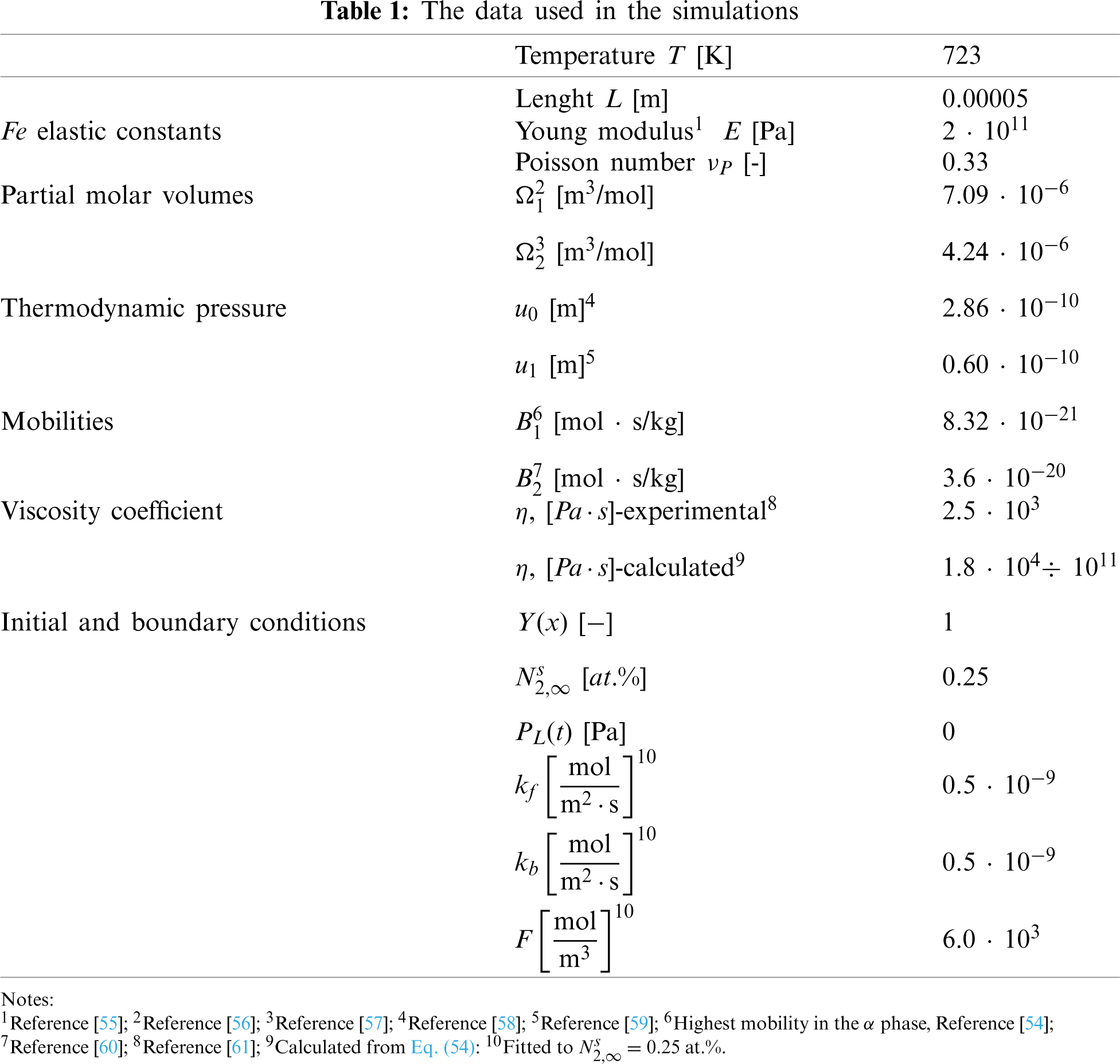
The programming has been performed using the Chesbyshev-Gauss-Lobatto and power grids. In Fig. 1, we show that the results don’t depend on the choice of the grid. Therefore, we have arbitrarily decided to perform the remaining computation using the program based on the power grid.

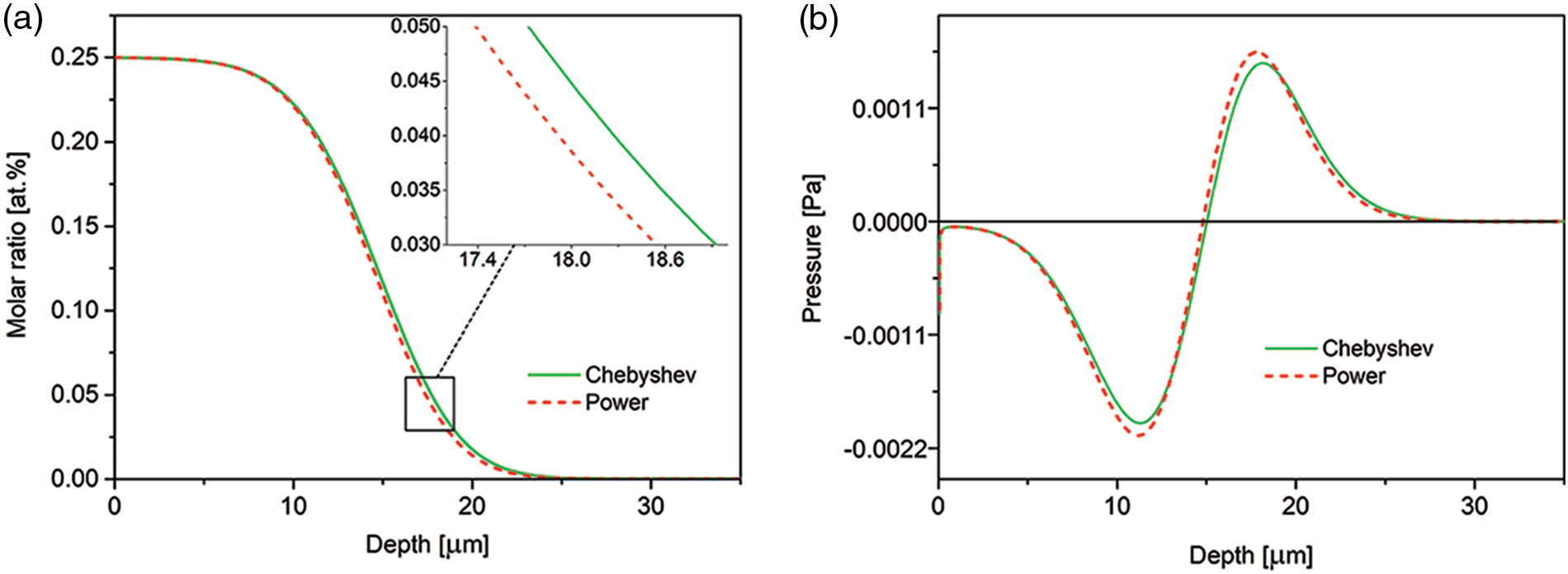
Figure 1: Comparison of the nitrogen concentration-depth profiles (a) and spatial pressure distribution (b), computed using the Chesbyshev-Gauss-Lobatto and power grids. The results after 15 h of the nitriding. The data simulated for the Dirichlet BC and experimental viscosity coefficient

In Fig. 2a comparison of simulations made for the two types of boundary conditions for nitrogen concentration at the open boundary is presented. We consider the Dirichlet and Chang-Jaffé boundary conditions. Although in the case of the Chang-Jaffé condition, the nitrogen concentration at the open boundary is calculated in the self-consistent way, without assuming given values, the both curves clearly overlap. The results also show that the concentration profile after 30 min of the processing exhibits an inflection, which at longer times transforms into a plateau characteristic for the non-Fickian diffusion in the expanded austenite.

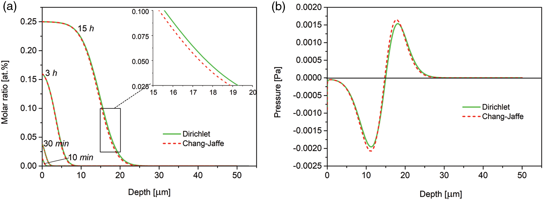
Figure 2: (a) Time evolution of the nitrogen concentration-depth profiles simulated with the use of the Dirichlet and Chang-Jaffé boundary conditions for the nitrogen concentration at the free left boundary Λ1(t); (b) spatial pressure distribution after 15 h of the processing. The data for the experimental viscosity coefficient

An effect of partial molar volume (here partial molar volume of nitrogen) is presented in Fig. 3, where we show the nitrogen concentration and pressure after 15 h of the processing. The assumed values are: Ω2=4.24⋅10−6 m3/mol--according to Jesperson [57] and Ω2 = 1.73 · 10−5 m3/mol--according to ChemGlobe. It is seen that the variation of the Ω2 affects mainly a case depth while the characteristic plateau does not dissappear. This fact confirms the validity of our model.

Figure 3: (a) Time evolution of the nitrogen concentration-depth profiles simulated for the nitrogen partial molar volume Ω2 = 4.24 · 10−6 m3/mol given in [57], and the nitrogen partial molar volume Ω2 = 1.73 · 10−5 m3/mol given in https://chemglobe.org/ptoe/; (b) spatial pressure distribution after 15 h of the processing. The data simulated for the Dirichlet BC and experimental viscosity coefficient

When we assume the Fe mobility equal to that at 723 K [54], B1=1.66⋅10−22 mol⋅s/kg, the results are qualitatively different. The plateau disappears and the sample becomes elongated, Fig. 4. Pressure distribution is also qualitatively different. It is because the computational time is too short for such a small mobility B1. For the plateau to appear, the time would have to be around 1500 h.

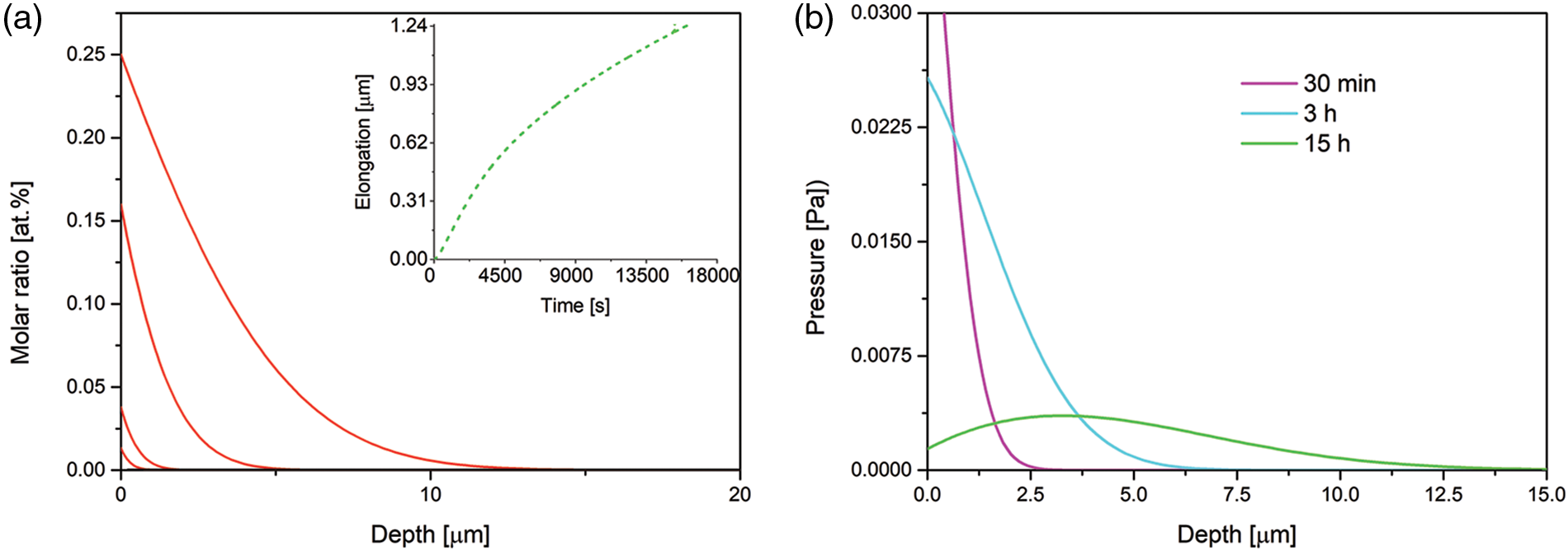
Figure 4: Time evolution of the nitrogen concentration-depth profiles (a) and spatial pressure distribution (b), simulated for B1 = 1.66 · 10−22 mol · s/kg (the Fe mobility in 723 K). The profiles after 10, 30 min, 3 and 15 h of the nitriding. The data simulated for the Dirichlet BC and experimental viscosity coefficient

In Fig. 5, the results for 4 samples of different thicknesses are presented. It is seen that the amount of the nitrogen dissolved and the case depth decrease when the layer thickness increases, Figs. 5e–5f. The observed differences are due to various stress distribution in the samples of various thicknesses. The pressure changing with the depth (pressure gradient) implies an additional driving force for the diffusion. It is seen that the pressure gradient decreases at longer times.

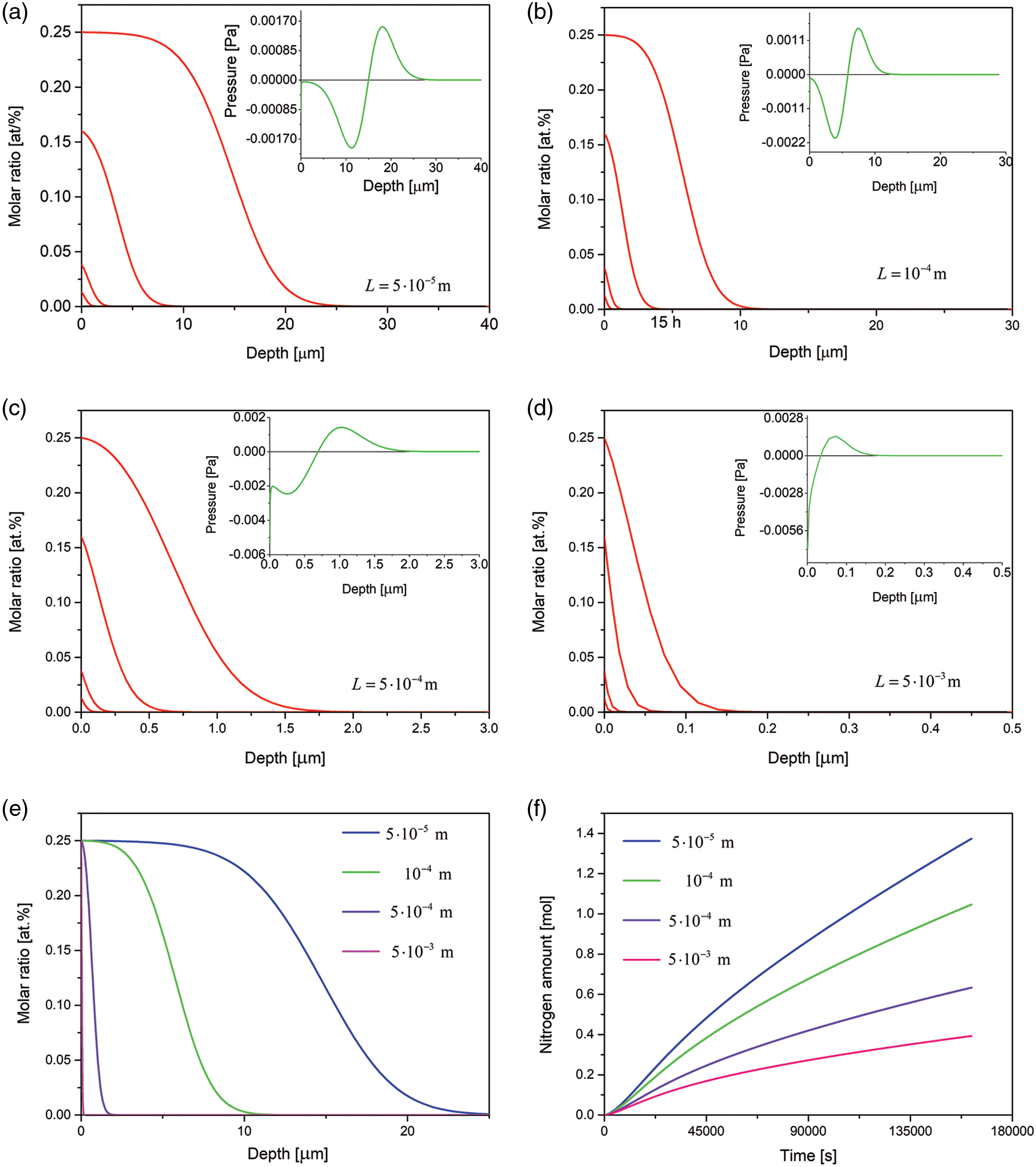
Figure 5: (a–d) Time evolution of the nitrogen concentration together with the spatial pressure distribution (in insets) simulated for the samples of various thicknesses, the respective profiles after 10, 30 min, 3 and 15 h of the nitriding; (e) comparison of nitrogen concentration profiles after 15 h of the nitriding of the samples of various thicknesses; (f) amount of nitrogen dissolved in the samples vs. time. The data simulated for the Dirichlet BC and experimental viscosity coefficient

Only quantitative differences are seen when the final nitrogen concentration at the open boundary is increased from 0.25 at.% to 0.35 at.%, Fig. 6.

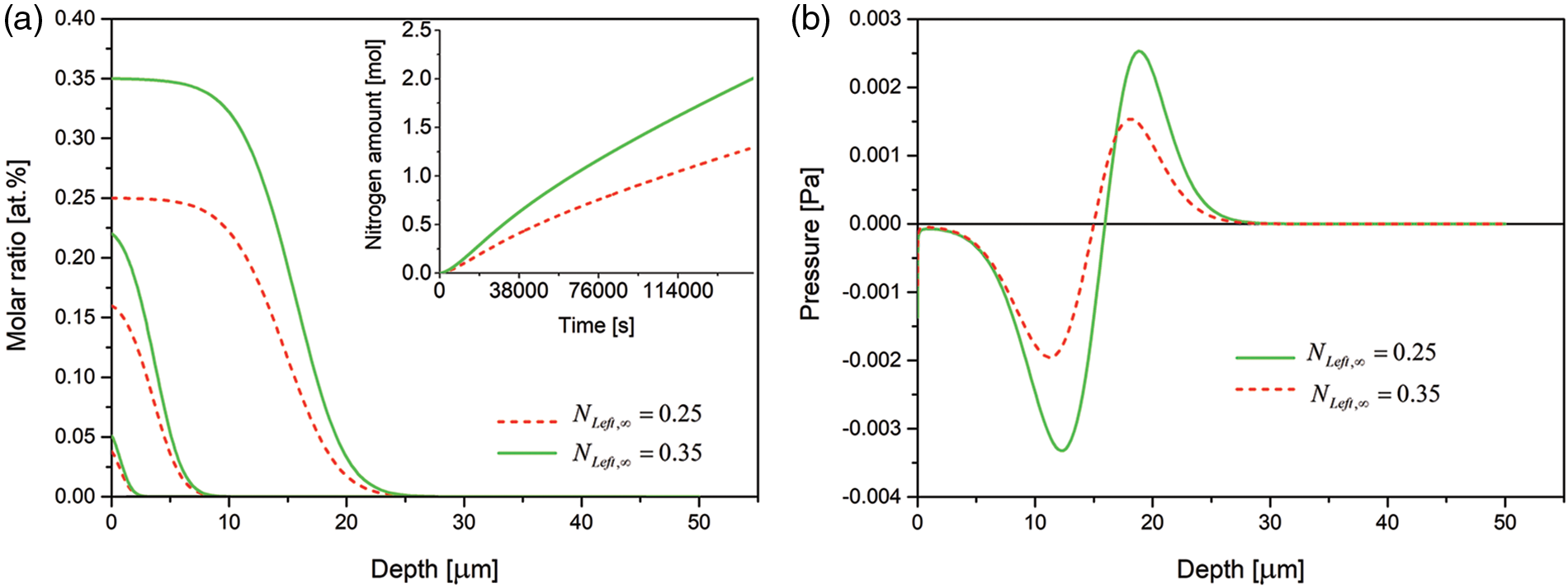
Figure 6: (a) Time evolution of the nitrogen concentration together with nitrogen dissolved (in inset) and (b) spatial pressure distribution for various steady-state nitrogen concentrations at the free left boundary Λ1(t), 0.25 and 0.35 at.%. The respective profiles after 30 min, 3 and 15 h of the nitriding. The data simulated for the Dirichlet BC and experimental viscosity coefficient

The effect of viscosity coefficient is presented in Fig. 7. It is seen that with increasing viscosity coefficient the case depth decreases and less nitrogen is dissolved in the substrate.

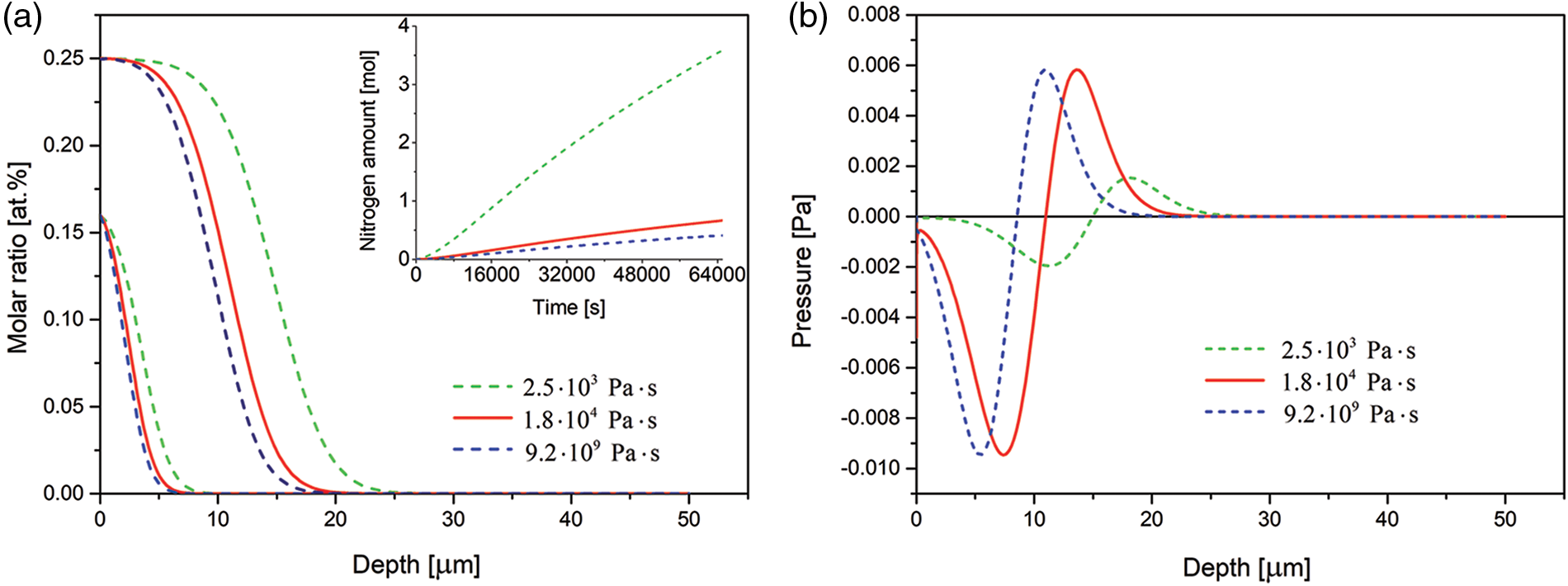
Figure 7: (a) Time evolution of the nitrogen concentration together with nitrogen dissolved (in inset) and (b) spatial pressure distribution simulated for the 3 samples of various viscosity coefficients. The respective profiles after 3 and 15 h of the nitriding. The data simulated for the Dirichlet BC

The presented results show that the appearance of the plateau at the nitrogen concentration profiles is conditioned by the mobilities of the species. It appears when the Fe mobility is higher than that at 723 K. Such processing can be realized in plasma conditions. The sample elongation is not observed. Qualitatively different results are obtained when assuming Fe mobility at 723 K (about 5 orders lower). No plateau appears and the sample becomes elongated. The characteristic plateau-type shape of the N-concentration depth profile has been confirmed by many authors [4,21,28]. Christiansen et al. in [20–22,28] studied the effects of in-depth stress gradients in expanded austenite. The obtained profiles showed a clear plateau followed by a steep nitrogen concentration decrease. Our results agree well with these results. Also, the experimental data measured by electron probe microanalysis (EPMA) in AISI 316 steel after low-temperature nitriding (440°C) for 23 hours at the nitriding potential KN=1.41 bar−1/2 (at which the surface nitrogen concentration is 0.25 at.%) and presented in [22] (Fig. 4) show the validity of the calculated profiles. By comparing the thickness of the nitride zone, our simulation provides an overestimate. The validity can be improved by adopting concentration-dependent diffusivity.

4  Summary and Conclusions

Low and intermediate-temperature nitriding of iron and stainless steel can cause a formation of expanded austenite phase. In this research, a formation of expanded austenite is modeled using the Darken bi-velocity method combined with the Vegard rule, the Maxwell model of viscoelastic solid, and the Gibbs-Duhem equation. It is the first such approach, which takes into account the interdiffusion of all components in the solid alloy. The model is formulated in any dimension and is given by a differential-algebraic system of 5 equations. In the one dimensional case, this system is equivalently transformed to the differential system of 2 equations only, which from analytical point of view is better to be studied. Effective mixed type boundary conditions are given. Such a nonlinear strongly coupled parabolic-elliptic differential initial-boundary Stefan type problem is solved numerically. A series of simulations is made. The results confirm an appearance of the characteristic plateau on the nitrogen concentration-depth profiles which is in agreement with literature data (see for example [20–22,28]). The model can be improved by the way of using concentration dependent diffusivities. It can be concluded that:

•   The nitrogen transport during nitriding is advanced by means of the stress and strain assisted interdiffusion.

•   The stress enhances the diffusion.

•   The interdiffusion can cause an imbalance in the volume transport and a non-uniform stress-free strain.

•   The stress and strain depend on the components’ mobilities, viscosity coefficient and thickness of the substrate.

•   Relaxation of the internal stresses generated by unbalanced diffusion fluxes can become the rate-limiting step for the interdiffusion.

The Maxwell model is usually applied to the case of small deformations. For the large deformations one should include non-linearity, e.g., the upper-convected Maxwell model. It can be further improved by the way of using concentration dependent diffusivities.

The initial boundary value problem presented here can be extended and even used in practical applications.

Funding Statement: This work has been supported by the National Science Center (Poland) Decision No. UMO-2013/11/B/ST8/03758 and by the Faculty of Applied Mathematics AGH UST statutory tasks within subsidy of Ministry of Science and Higher Education (Grant No. 16.16.420.054). Research data are referenced in Section 3.4. They will be available on requirements.

Conflicts of Interest: The authors declare that they have no conflicts of interest to report regarding the present study.

Appendix A

To express the chemical potential gradient ∂μ1∂x as a function of y1, let us notice first that N1=c1c, y1 = Ω1c1, Ω1c1 + Ω2c2 = 1 and c1 + c2 = c. We can write:

c=Ω1+(Ω2−Ω1)y1Ω1Ω2, (55)

N1=Ω1c1Ω1c=y1Ω1c=Ω2y1Ω1+(Ω2−Ω1)y1, (56)

∂N1∂x=Ω1Ω2(Ω1+(Ω2−Ω1)y1)2∂y1∂x. (57)

After introducing (56) and (57) into (39) leads to (40).

Appendix B

We want to find a differential equation on the pressure P. The formulas (38) and (40) imply the relation

∂∂x((B1y1−B2(1−y1)c1c2)RTΩ1y1(Ω1+(Ω2−Ω1)y1)θ1∂y1∂x)+∂∂x((Ω1B1−Ω2B2)y1∂P∂x+Ω2B2∂P∂x)=1η∗P. (58)

It follows from elementary calculations that

B1y1−B2(1−y1)c1c2=B1y1−B2(1−y1)c1Ω1Ω2c2Ω1Ω2=Ω1B1−Ω2B2Ω1y1. (59)

By inserting (59) to (58) we have

RT(Ω1B1−Ω2B2)∂∂x(1Ω1+(Ω2−Ω1)y1θ1∂y1∂x)+(Ω2B2+(Ω1B1−Ω2B2)y1)∂2P∂x2+(Ω1B1−Ω2B2)∂y1∂x∂P∂x=1η∗P (60)

and equivalently

(Ω2B2Ω1B1−Ω2B2+y1)∂2P∂x2+∂y1∂x∂P∂x−1(Ω1B1−Ω2B2)η∗P=−RT(θ1Ω1+(Ω2−Ω1)y1∂2y1∂x2+∂∂x(θ1Ω1+(Ω2−Ω1)y1)∂y1∂x). (61)

In fact Eq. (61) is identical with Eq. (41).

Appendix C

We will show that

Ω1J1+Ω2J2=0. (62)

It follows from (8) that

Ω1J1+Ω2J2=K(t), (63)

by one dimension n = 1. Let Jid=−Bici(∂μi∂x+Ωi∂P∂x) mean the diffusion terms of the fluxes Ji, i = 1, 2 given in (1). Because at the right boundary v(t, Λ2) = 0 and Ω1J1d(t,Λ2)+Ω2J2d(t,Λ2)=0, then K(t) ≡ 0 and in consequence (62) is satisfied.

Appendix D

We will construct implicit finite difference methods for the system (42) with the initial condition (45) and two types of boundary conditions: (46)–(48)-the Robin type, and (46), (47), (53)-the generalized non-local Robin type, respectively. These numerical methods are generated by some linearization and spliting ideas. The date used in simulations are given in Table 1. To avoid a double indexation, we put: y: = y1 and θ: = θ1.

Define a mesh on the set [0, ∞) × Σ(t) = [Λ1(t), Λ2] in the following way. Let τ > 0 stands for the time step of the mesh and define nodal time points tν = ντ, ν∈N∪{0}. Let moreover M∈N be given, Λ1ν=x0ν<x1ν<…<xMν<xM+1ν=Λ2 be at this moment arbitrarily fixed nodal space points and let hmν=xmν−xm−1ν,m=1,…,M+1 mean the space steps of the mesh. Define new nodal space points x¯mν=xm+12hm+1,m=0,…,M. Note that x¯mν−x¯m−1ν=hm+hm+12. Put ℏmν=hmν+hm+1ν2.

For the left end of the domain Σ(t), the approximation of (44) is applied,

Λ1ν+1=Λ1ν−τ2η∗∑m=1M+1hmν(Pm−1ν+1+Pmν+1),Λ10=0. (64)

Two definitions on the space nodal points will be used in computations:

xmν=Λ1ν+(mM+1)s(Λ2−Λ1ν),m=0,…,M+1, (65)

for s = 3/2 or s = 2;

xmν=Λ1ν+1+cos⁡(2M+4−m2M+4π)1+cos⁡(M+32M+4π)(Λ2−Λ1ν),m=0,…,M+1. (66)

Eq. (65) describes the power and Eq. (66), the Czebyshev–Gauss–Lobatto grids.

We define two linear implicit difference schemes: for the ordinary equation on pressure P and for the parabolic equation on concentration y1 in system (42) with the initial-boundary conditions (45)–(48). For each ν, they are algebraical systems of M+1 equations with M+1 unknowns of the form

{ym0=Y(xm),m=0,…,M+1,P00=PL(0),Am−10Pm−10+Am0Pm0+Am+10Pm+10=G(ym0),m=1,…,M,PM+10=PM0, (67)

{C0ν+1=YL(tν+1),Cm−1ν+1ym−1ν+1+Cmν+1ymν+1+Cm+1ν+1ym+1ν+1=ymν,m=1,…,M,CM+1ν+1=CMν+1, (68)

{Pmν+1=PL(tν+1),Am−1ν+1Pm−1ν+1+Amν+1Pmν+1+Am+1ν+1Pm+1ν+1=G(ymν+1),m=1,…,M,PM+1ν+1=PMν+1, (69)

where

Am−10=1ℏm0(S(ym0)hm0−14ℏm0(ym+10−ym−10)),

Am0=−S(ym0)ℏm0(1hm+10+1hm0)+Q,

Am+10=1ℏm0(S(ym0)hm+10+14ℏm0(ym+10−ym−10)),

S(ym0)=Ω2B2Ω1B1−Ω2B2+ym0,

G(ym0)=−RT(θm0Ω1+(Ω2−Ω1)ym01ℏm0(ym+10−ym0hm+10−ym0−ym−10hm0)

+(θm+10Ω1+(Ω2−Ω1)ym+10−θm−10Ω1+(Ω2−Ω1)ym−10)ym+10−ym−104(ℏm0)2)

≈RT(−θm0Ω1+(Ω2−Ω1)ym01ℏm0(ym+10−ym0hm+10−ym0−ym−10hm0))

+RT((Ω2−Ω1)θm0(Ω1+(Ω2−Ω1)ym0)2(ym+10−ym−102ℏm0)2),

Am−1ν+1=1ℏmν(S(ymν+1)hmν−14ℏmν(ym+1ν+1−ym−1ν+1)),

Amν+1=−S(ymν+1)ℏmν(1hm+1ν+1hmν)+Q,

Am+1ν+1=1ℏmν(S(ymν+1)hm+1ν+14ℏmν(ym+1ν+1−ym−1ν+1)),

S(ymν+1)=Ω2B2Ω1B1−Ω2B2+ymν+1,

G(ymν+1)=−RT(θmν+1Ω1+(Ω2−Ω1)ymν+11ℏmν(ym+1ν+1−ymν+1hm+1ν−ymν+1−ym−1ν+1hmν)

+(θm+1ν+1Ω1+(Ω2−Ω1)ym+1ν+1−θm−1ν+1Ω1+(Ω2−Ω1)ym−1ν+1)ym+1ν+1−ym−1ν+14(ℏmν)2)