Computer Modeling in Engineering & Sciences

DOI: 10.32604/cmes.2022.017030

ARTICLE

ResNet50-Based Effective Model for Breast Cancer Classification Using Histopathology Images

Nishant Behar* and Manish Shrivastava

Department of Computer Science & Engineering, GGV, Bilaspur, 495009, India
*Corresponding Author: Nishant Behar. Email: nishant.itggvonline@gmail.com
Received: 26 April 2021; Accepted: 11 August 2021

1  Introduction

The International Agency for Research (IARC), a part of the World Health Organization (WHO), coordinates and conducts both epidemiological and laboratory research into the causes of human cancer; it reported that breast cancer is the most commonly occurring cancer worldwide (11.7% of the total new cases). In the projected burden of cancer in 2040, it was estimated that in 2.3 million new cancer cases worldwide, one in every 8 cancers diagnosed in the year 2020 will turn out to be breast cancer; it is the fifth leading cause of cancer mortality worldwide, with 685,000 deaths in the year 2020. In women, breast cancer ranks first in terms of incidence and mortality in most countries around the world [1]. This high mortality rate can be reduced through timely detection of the disease, in its early stages. The manual detection method, fine needle aspiration (FNA), is a simple and quick cytology procedure to discover cysts or cancer, by examining the fluid characteristics extracted from the suspected area; however, the diagnosis processes are subject to expert inferences on visual anomalies. This pathological challenge, associated with FNA, encourages researchers to discover a new, automatic, quick and consistent method to analyse and detect cancerous cells. The last decade has witnessed steady progress of the convolutional neural network (CNN), which represented significant contribution towards automated detection of tumour images and provides additional support to healthcare experts, allowing them to make accurate decisions. Therefore, research developments are focused on computer-aided diagnostic (CAD) methods for disease prognosis and diagnosis purposes. In CNN, breast cancer diagnosis is carried out by examining the images acquired through different medical instruments like mammograph, breast ultrasound, magnetic resonance imaging (MRI) or the open biopsy process. A typical CAD system has four common steps: (a) input images, (b) pre-processing, (c) feature extraction and (d) classification; after these steps, results are produced. A specialized artificial neural network (ANN) model—CNN—includes all the above-mentioned steps.

ANN techniques have become popular among researchers due to their excellent learning ability and built-in parameter tuning mechanism. As a result, ANN is widely used to examine theoretical and applied science models. To study and determine the behavior of any model, correct mapping between inputs and the target parameters of the model is an essential step. ANN methods play a key role in modifying crucial internal parameters and providing an optimized network weight. Some recent studies have described the use of an ANN method alone or in conjunction with genetic algorithm (GA), particle swarm optimisation (PSO), whale optimization algorithm and sequential quadratic programming (SQP), to simulate well-known multi-disciplinary equations. In the studies [2–6], Emden-Fowler model for its second and third order systems has been solved successfully. In other studies [7,8], Lane-Emden delay differential model was analysed. Several authors have used conventional mathematical simulations like fractional dynamics behaviours using Chebyshev polynomials converted into a linear equations [9], masses on the vertices of equilateral triangle [10] and modelling of human liver with the Caputo-Fabrizio fractional derivative [11] for their experimental models. Furthermore, researchers [12–16] presented mathematical modelling in some different areas and have claimed that their proposed algorithms can be suitably applied in diverse fields. Moreover, ANN has evolved as a promising technique in the healthcare sector for diagnoses and processing medical images.

In our present study, an ANN technique was implemented for adjusting network weights recursively for minimizing detection errors. In the prior reported work [17], researchers have proposed a dataset and applied a two-class computer-based classification; they obtained accuracy within the ranges of 80% to 85%. With this background, this study aims to propose an effective classifier with high classification rate and accurate detection of malignant and benign tumours from breast histopathology images. Some images of benign and malignant tumours are shown in Fig. 1.

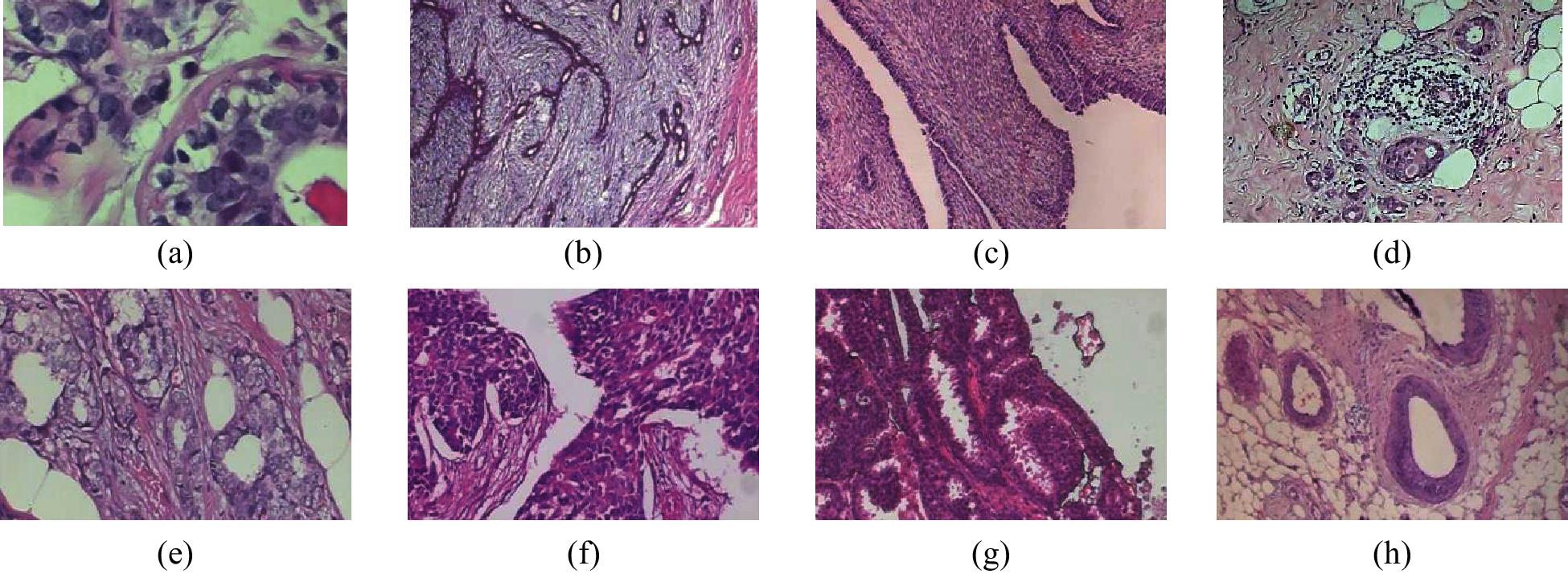
Figure 1: Different breast cancer biopsy images [17]. (a–d) Benign tumour images. (e–h) Malignant tumour images

The prime objective of this study is to provide an effective model, with a high accuracy rate, for the classification of cancerous and non-cancerous images. The remaining sections are organised as follows: Section 2 is dedicated to the literature review, Section 3 introduces the CNN concepts, Section 4 describes research methodology with experimental outcomes and Section 5 concludes the study and unfolds further research opportunities.

2  Literature Review

This literature review includes the research papers that used pre-trained systems for breast cancer classification. Some substantial and relevant studies have been discussed in this section.

In a study, researcher have developed a deep feature-based model (DeCAF) [18], for the classification of breast histopathology images, and the pre-trained BVLC Caffenet model, which is available for free in the café library, was implemented as a feature extractor. Various outputs obtained from different fully connected layers were analysed individually and in different combinations. Logistic regression was used as a base classifier for the evolution of these deep features. The experimental outcome has exhibited a high accuracy rate and better performance than hand-made features for image recognition. In an experimental work [19], a transfer-learning method was employed to classify histopathological images, and a pre-trained CNN was used to encode the local features into Fisher vector (FV). Authors also introduced a new adaptation layer that enhances discriminant characteristics of features and improves classification accuracy. VGG-VD was implemented for accomplishing transfer learning. The study [20] presented a classification scheme to generate and assign confidence score to images of each class. The classification was based on the Kernel principal component analysis (KPCA) ensemble method, and the proposed scheme was successfully tested on two different datasets: (a) breast cancer and (b) optical coherence tomography. This study has also imposed a research challenge to find an optimiser, to reduce the fixed size parameters applied in this work. In the reported work [21], 1.2 million high-resolution images have been categorised in 1,000 different classes through a large, deeper and focused neural network in the ImageNet (LSVRC-2010) competition. This novel model consisted of 60 million parameters, 650,000 neurons and five convolution stages. The fully connected layers applied the SoftMax function. Experiment outcome reported the lowest error rates of 37.5% and 17.0%, respectively. The research work [22] provides an automatic two-step classifier for slide investigation. In the first step, coarse regions were analysed in the whole slide to obtain diverse spatially localised features, after which the detailed analysis of the selected tiled region was completed. This experiment used elastic net classifier and weighted voting classifier for cancer detection on brain image dataset. The research paper [23] presented a probabilistic classifier that combines multiple-instance learning and relational learning. The instance-based learning was used for the classification task, whereas relationship-learning map was used for the changes in the cell formation due to cancer. This approach had been evaluated on breast and Barrett's cancer tissue microarray datasets. In another work, the researcher had developed an accurate, reliable, and multistage method for measuring the neoplastic nuclei size for pleomorphism grading [24]. In the preliminary stage, image quality, staining value and tissue appearance were observed. In a later stage, machine-learning methods were used to score and remove abnormality that existed in nuclear contour, for better segmentation. A study has discussed difficulties associated with multiclass classification due to broad variability, high coherency, and inhomogeneity of colour distribution. In this paper, authors had resolved these issues and proposed a breast cancer multi-classification method, which used a structured deep-learning model [25]. This model includes a training stage, extracting features and optimises inter-class distances. The validation stage was used for parameter tuning, while the testing stage comprised model evaluation. The final accuracy was obtained as 93.2% for multi-class binary classification on the breast biopsy image dataset. A study has addressed an intra-embedding supervised classification method to classify histopathology images; in this innovative work [26], Fisher encodings are embedded with CNN architecture. The results of the work concluded that the proposed method can successfully resolve the issues of high dimensionality and busty visual components, which are associated with FV. This model was evaluated in lymphoma and breast cancer datasets, where highest classification accuracies on different magnification levels were reported on the breast cancer histopathology dataset. An experimental work [27] was focused on the use of colour-textural characteristics of the breast cancer histopathology images, for effective classification. In this work, different classifiers, namely support vector machine (SVM), decision tree, nearest neighbour and discriminant analysis, were included for creating an ensemble classifier. The proposed model was studied on various optical magnification levels, to acquire better discriminative features. A CNN-based approach was applied in [28], where patch-level classifications were carried out on breast cancer biopsy images. The maximum accuracies reported 77.8% for four classes and 83.3% for two classes, for instance, carcinoma/non-carcinoma through the CNN-SVM model. Another approach [29] had examined 74 features and their importance was inferred, based on pixel level, contrast and texture. Additional features were also studied like geometry and context for significant contribution, to achieve a better accuracy rate. In the novel work [30], researchers have applied CNN for correct detection of smoke in a region from video frames.

Based on earlier research work, it can be summarised that the use of machine-learning methods, especially deep learning algorithm, can be efficiently optimised for cancer cell detection, segmentation and classification. Review of literature also highlighted the importance of input image quality, feature extraction and classifier for development of an effective computer-based system. A lot of contributions have already been made in the recent years, but there is always scope for achieving better classification accuracy, which is the basis of our research work.

3  CNN Architecture

Automatic feature extraction is the prime benefit of using CNN. This concept was originated through experimental work done by Hubel et al. [31] in 1968. They had analysed the cortex responses on different light intensities for simple, complex and hypercomplex patterns. Based on this concept, Fukushima [32] had proposed a “Neocognitron” neural network process model to recognise visual patterns, using the “learning-without-a-teacher” concept. This model applies the novel S-layer and C-layer. The S-layer portrayed geometrical features, and the C-layer was applied to down-step the S-output, by responding selectively for a single-stimulus pattern. CNN architecture is more complex due to multiple layers, which implement a convolution operation to extract local and global features, to determine the underlying pattern of an image. Extracted features are extremely useful; they guide the network towards the learning direction and lead to automatic decision-making. CNN model has another important layer—pooling layer—which reduces the dimension received from the previous layer. In a single CNN architecture, there can be many combinations of convolution and pooling layers. These intermediate layers are used to identify spatial visual patterns from images, as shown in Fig. 2. These convolution and pooling layers are discussed in Subsections 3.1 and 3.2, respectively.

Figure 2: Schematic diagram of typical CNN architecture

3.1 Convolution Layer

The key function of the CNN model is executed by its convolve layer, which significantly identifies the different shapes of the input image, using different filters (or kernels). More specifically, one filter can only detect one pattern; therefore, multiple filters are generally used to determine complete image components. To understand the convolution process, for example, an n * n size image and an m * m size filter (such as m = 1, 3, 5…and m < n) are fed to a convolution layer such that the filter slides over the image to form an m * m image region. For this image region, a dot operation takes place between corresponding pixels of the filter and the specific image region. The result of this operation provides most valuable pixel information, which expresses a particular pattern. The mean of all m * m pixels is calculated, which is stored in a single-cell output matrix (i.e., feature map). This process is repeated until the filter slides on every possible location over the image. Once the whole process is complete, the feature map is generated. Two important methods, stride and padding, also affect the feature map result during this convolution process. A stride ‘s’ determines the value of jump or movement of the filter from current location to next location over the image; generally, the values are s = 1, 2 or 3, whereas padding adds some additional rows and columns in an image with the pixel value = 0. Padding ensures the proper representation of corner and edge pixel values in the feature map. This feature maps are fed to the next layer, as illustrated in Fig. 3.

Eq. (1) is expressing the mathematical operation performed during the convolution process. Suppose Xi,j is the height and width of an image region and Fv1,v2 is filter used in a convolution process, where v1 = v2, filter size is Fv1,v2 < X i,j and ∗ is a dot operator, then each movement of the filter over the particular region of image (i.e., m * n) involves two actions: (a) dot operation: the pixel-wise dot operations are performed between the specific pixels of the selected image region and the corresponding pixel of the applied filter and (b) summation: all resultants are summed together to form a single input value, to contribute a cell value in the feature matrix. Following expression with bias, provides the complete feature matrix that can be referred [33].

Inputimage(Xi,j)∗Filter(Fv1,v2)=(∑m=−v1+12v1−12⁡∑n=−v2+12v2−12⁡Xi−m,j−n∗Fm,n)(1)

Figure 3: Illustration of convolve process

The size of convolutional layer can be defined as Eq. (2), where input size (R), Filter size (F), padding (p) and stride (s) are used in a particular layer:

Featuremapoutputsize(o)=(R−F+2p)s+1(2)

3.2 Pooling Layers

Pooling layer is the crucial next stage; it comprises decreasing the matrix size of the convolution layer. Pooling layers are arranged just after one or more convolution layers so that it can retain the most significant values from feature map. Two popular pooling methods are max pooling and average pooling. The max pooling method contains only the maximum value from a specific sub matrix (i.e., m * n) of the feature map; average pooling collects the mean value of the feature submatrix, which can be referred to in Eq. (3) [34].

Pijq=max(m,n)∈Fi,j Pmnq(3)

Here, Fi,j is a complete feature matrix of a particular layer ‘q’, and Emnq are matrix elements on the feature map submatrix (m*n). Once this process is complete for all possible subregions of the feature map, the complete downsized output matrix can be obtained for further processing.

3.3 Classification Layer

3.3.1 The Classifier

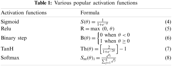
Classification refers to assigning a single label to an unknown sample in the pool of different classes, whereas a classifier is a mathematical function applied to learn the underlying hidden patterns from the training dataset such that the input data can be mapped with their actual label. Once learning is complete, the classifier is used to predict unlabelled data. A fully connected (FC) ANN is usually applied as a classifier, followed by the flatten layer. This FC layer contains collection of nodes, like human brain neurons, and they are arranged in multiple layers of input, hidden and output. All nodes of one layer are linked with every node of the next layer. The final feature vectors are forwarded to this FC network, and input layers of the FC network are fed forward to the subsequent hidden layer. Every node of each layer has some specific weight; it is multiplied with the prior layer output and added with the bias values of its own layer. The last layer determines the most suitable class for the input image, and each node has its own summation and activation function. The activation function is a mathematical process which decides whether a node value needs to be activated (or triggered) or not for the prediction purpose, based on some predefined threshold value. The most popular activation functions are binary step (B), sigmoid (S), relu (R), tanH (Th) and SoftMax (Sm). The following Table 1 summarises some of the functions, with Eqs. (4)–(8).

3.3.2 The Cost Function

The cost function represents the learning ability of a classifier. It represents the gap between predicted and actual class of input dataset; this gap should be minimum. A counter feedback (i.e., backpropagation) process is employed to re-adjust neuron weights of all hidden layers in the opposite direction. After tuning the network weight, the updated cost value is checked, and gaps are analysed again. This learning process is repeated until and unless the optimum value, in the form of global minima, is achieved and the network classifies the maximum correct labels for given dataset. The cost function can be mathematically expressed as Eq. (9)

Cost(C)=1M∑i=1M⁡(Y^i−Yi)2(9)

where X is the set of input samples {X1, X2…XM} and Y is the corresponding true labels {Y1, Y2….YM} of X. The total number of samples are M and the predicted output label (Y^i) for sample ‘i’ is such that Y^i\; =f(Xi).

4  Research Methodology

4.1 Breast Cancer Dataset

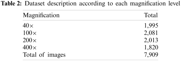
In this study, we have used a BreakHis open dataset, which contains different breast cancer classes in two main categories, benign and malignant. A total of 7,909 images of 40×, 100×, 200× and 400× magnification levels were obtained from 82 patients. Out of these, 2,480 belonged to the benign and 5,429 to the malignant class. Each image has been represented by an 8-bit RGB channel, with the size of 700 × 460 pixels. Total number of images, based on different magnification levels, are summarised in the Table 2.

The benign tumour is further sub-classified into adenosis, fibroadenoma, phyllodes and tubular adenoma. Malignant tumour type is sub-categorised into ductal carcinoma, lobular carcinoma, mucinous carcinoma and papillary carcinoma. In this experimental work, all images have been manually partitioned into benign or malignant; this allows the problem to be formulated into binary classification. Data augmentation has also been applied due to lesser number of training data samples. The complete dataset was divided into training (6327 images), validation (790 images) and test subsets (792).

4.2 Proposed Model

In this experimental work, a multi-layered deep CNN framework Resnet50 was tuned for transferring the learning process. ResNet-50 is a prebuilt model which has been trained on the ImageNet dataset for identifying different images of 1,000 classes. ImageNet pre-trained weights were supplied as initial weights for the proposed deep neural network. The residual layers present in ResNet50 plays an important role, to transfer large gradient values to its prior adjacent layers. Due to this layer, the model can effectively extract complex and relevant patterns and resolve the vanishing gradient problem [35,36]. In our experimental setup, all pre-train model layers are kept open to learn new features from biopsy images. The feature matrices, acquired from CNN layers, were supplied to the fine-tuned FC layer, where the sigmoid function was used in the output layer. Further, the Adam optimiser was applied, with the learning rate 0.00001, for achieving better accuracy. The loss function was set to binary cross entropy. Loss function indicates the difference between the actual and predicted value. Epoch was set to 80. The available data were highly imbalanced in their sample number, so for the data balancing, proper weights for each class were assigned; please refer to Fig. 4. The whole dataset was divided into different subsets as follows: training dataset with 6,327 images to train the model, validation dataset has 790 images for tuning network parameters and test subsets have 792 images to evaluate model performance.

Figure 4: Indicating imbalanced dataset

The data augmentation has been applied additionally to generate flipped, zoom, shearing and scaling training datasets, whereas validation and test datasets have been only scaled. Images have been randomly selected from every category. The proposed architecture delivers an adequate performance with excellent accuracy and other model measures rates. Fig. 5 shows the flow chart of the proposed model.

4.3 Evaluation Parameters and Metrics

The utility of the model is mainly measured by accuracy rate of its classification. The confusion matrix is used to analyse the additional quality parameters like precision, recall and F1 score. A 2 * 2 confusion matrix represents performance measures for binary classification; it is inferenced in Fig. 6. Here, a different cell element contains the true positive (TP), false negative (FN), false positive (FP) and true negative (TN) values. The TP refers to correct prediction of true positive class, FP refers to the cases where there is an actual negative class—but it is determined as a positive class—TN is referred as the negative class correctly predicted and FN shows a positive class incorrectly as a negative class.

The accuracy outcome is an important measure for any CNN model. It represents the ratio of total correct prediction (TP + TN) over all predictions (i.e., TN + TN + FP + FN) generated by the model. Accuracy, precision, recall and the F1 score can be calculated from the equations, Eqs. (10)–(13).

Accuracy(A)=(TP+TN)(TP+TN+FP+FN)(10)

Precision(P)=TP(TP+FP)(11)

Recallortruepositiverate(TPR)=TP(TP+FN)(12)

F1score=2∗(Precesion∗Recall)(Precesion+Recall)(13)

Figure 5: Step-by-step illustration of proposed model process

Figure 6: Representing 2 * 2 confusion matrix for the binary classification

4.4 Experimental Results

This study was setup in Colab Notebook, offered by the google cloud platform, with a Tesla T4 GPU. Python and Keras, were used for the programming and model-tuning purposes. For performance evaluation, the Sklearn library [37] was employed, and conclusion was drawn from confusion matrices. This study consists of six major steps: (a) image pre-processing and data augmentation, (b) feature extraction, (c) network training and FC layer fine-tuning, (d) model accuracy evaluation using validation dataset, (e) finalisation of model and (f) final performance evaluation on accuracies and other parameters using unseen test data set, as presented in Fig. 5.

Image processing is an important step; it enhances the quality of image and prepares input images for network learning. Data augmentation was necessary due to lesser number of available images, which were further divided into train, validation and test datasets. Feature extraction has been carried out through the prebuilt model, Resnet50. The pre-trained weights were loaded initially, and the network layers have been kept trainable, allowing the model to learn new patterns from the provided unseen medical dataset. Fine-tuning was carried out through redefining the FC layer, and hyper parameters have been tuned by multiple runs for the optimum accuracy on training and validation dataset. Model training epochs were set as 80. Once the training was completed, the final accuracy on the test dataset was obtained. The experimental result projected exemplary training accuracy, 99.70%, and validation accuracy as 99.24%. Fig. 7a illustrates a graphical representation of the achieved accuracies for training and test datasets during 80 epochs. Fig. 7b determines model perfection, through the loss ratios obtained for training and validation as 0.190 and 0.0694, respectively.

Figure 7: Demonstration of training and validation samples (a) accuracies and (b) the loss values

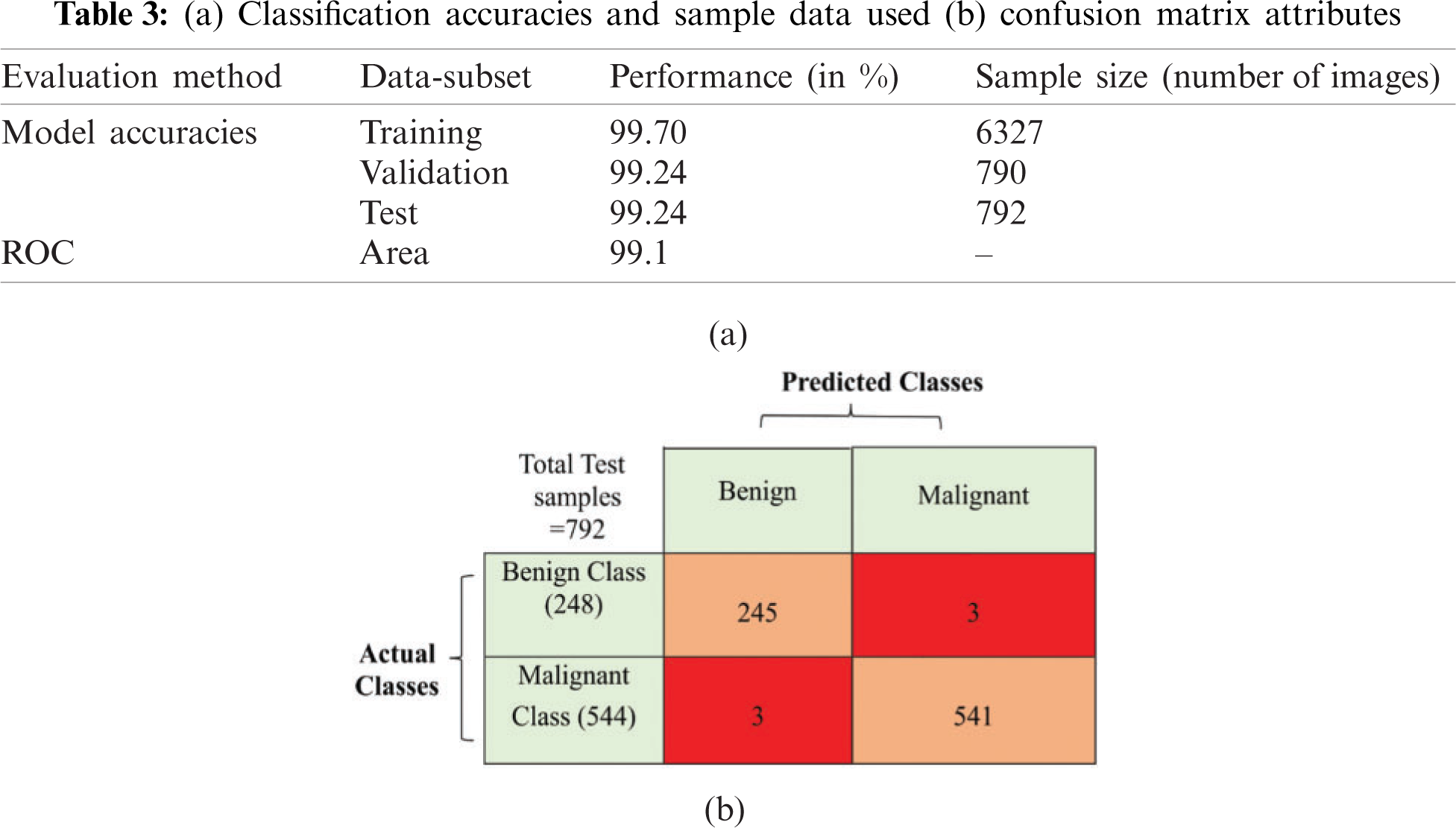
When the model was evaluated through untouched test dataset, encouraging results were found, with 99.24% accuracy and a loss value of 0.0491. Further, for deeper analysis of the model, confusion matrix and other evaluation parameters, such as precisions, recall, F1 score, were also carefully observed; this concluded that the model is correctly classifying each sample of different data subsets; refer to Tables 3a and 3b.

Receiver operating characteristics (RoC) analysis is a well-defined graphical representation to show the trade-off between true positive rate and false positive rate for binary classification tasks [38]. The area under the curve (AUC) is also important to determine model's capability, to distinguish between one class and another. In this experiment, RoC area was found as 99.1% as depicted in Fig. 8. This clearly indicates that the proposed model can classify input images into their correct class.

Figure 8: RoC curve and AUC evolution performed on test dataset

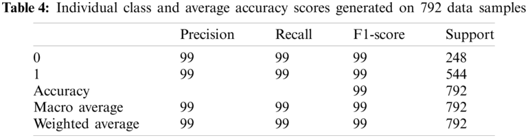
The individual class performance with precision, recall and F1-score is shown in Table 4. In this table, benign class is encoded as ‘0’ and malignant class is represented as ‘1’. Parameter ‘Precision’ depicts the proportion of TP values over total samples predicted for positive inclusion of FP—please refer to Eq. (11). Precision value is an important parameter, as it indicates unbiased and precise model performance for positive class predictions. ‘Recall’ parameter also represents the proportion of positive class over sum of predicted TP and FN samples—please refer to Eq. (12). F1-score represents harmonic mean of precision and recall value—please refer Eq. (13). The term ‘Support’ defines the class samples involved in this calculation. The higher values of accuracy, precision, recall and F1 indicate superior model performance.

The following Table 5 illustrates the comparative performance of the model in similar studies. In this comparison, only two-class classification on the same BreakHis dataset have been considered. The exemplary accuracy, precision and F1 score rate of our proposed model can be noticed. A comparative account of accuracy of model is depicted in Fig. 9.

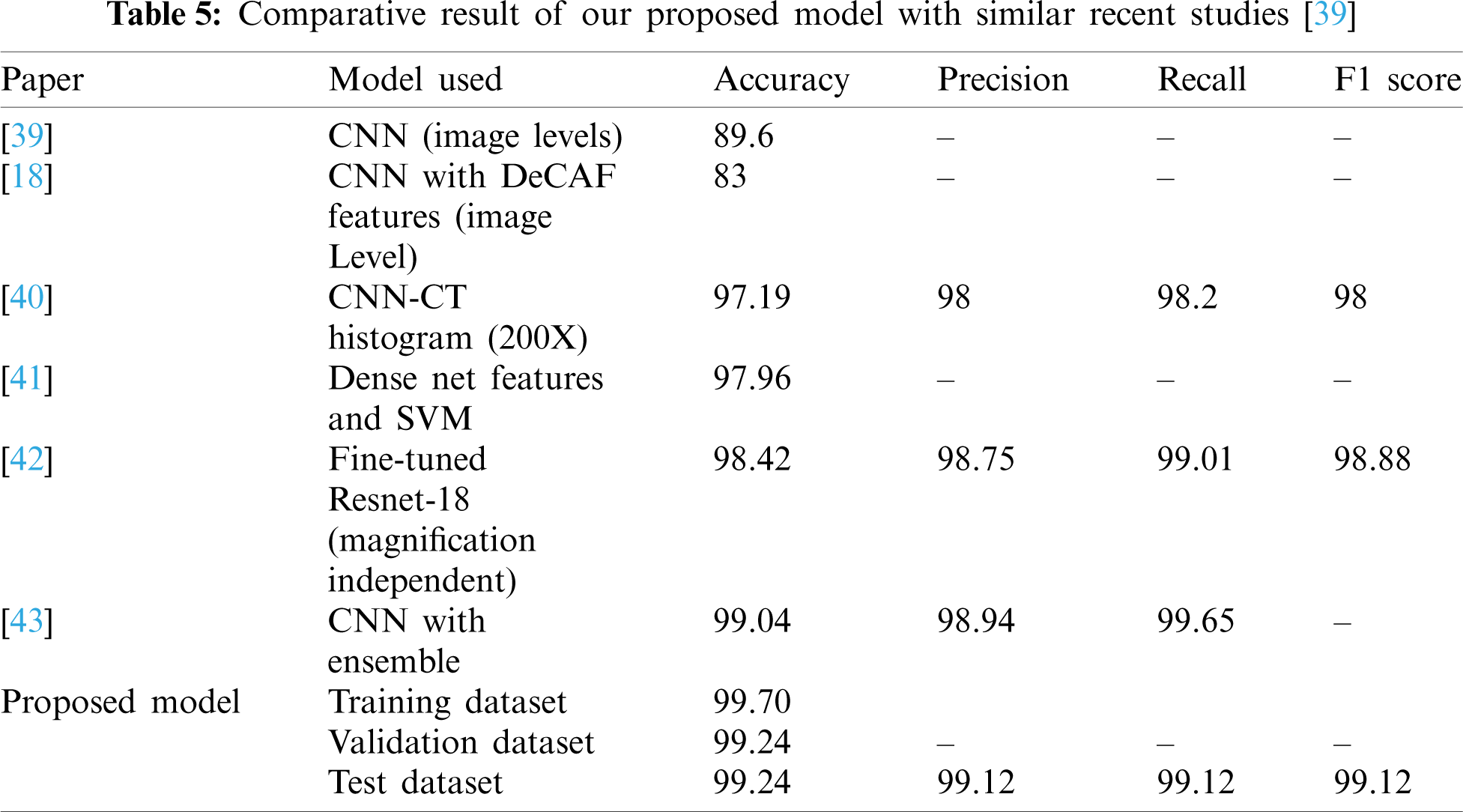
Figure 9: Illustration of accuracy performance of proposed model with latest similar work

5  Conclusion and Future Work

This study discussed the general functioning of the CNN model and proposed a model that was effective in the classification of cancerous and non-cancerous histopathology images taken from the Breakhis dataset. It was quite a challenging task to extract the prominent features due to variability in H&E stain, colour intensities, irregular shapes, high resolution and large sizes of images. Manual analysis of these images are always hard and time-consuming and are subject to the expertise level of specialists. Highly unbalanced and smaller sample images were another associated problem in the study; however, necessary steps, such as data augmentation and proper class weights, were taken to resolve these issues. The strength of our proposed model is based on the network’s learning ability and accurate classification capabilities of the BreakHis dataset. The extracted feature also adequately determines the complex local and global features of histopathology images, and supports the redesigned FC layer learning. For the evaluation of the proposed model, only calculating the accuracy parameter is not enough. Therefore, other performance measures—RoC, precision, recall and F1 score—have also been calculated; this allows true and reliable detection of image classification. The results were encouraging when compared with similar recent works. The regularisation and dropout values can be tuned further for better results; however, the testing results adequately prove that the proposed model is outperforming previous models, and it is appropriate for providing preliminary assistance to the healthcare experts for quick and accurate decision-making. Thus, a reliable and consistent CNN model based on pre-built Resnet50 architecture, which exploits the transfer learning technique, has been developed.

In future, this work will be extended to study one or more model parameters and their optimisation, like network complexity, image channels, computational time and space complexity. Furthermore, experiments for the multiclass classification on same dataset will/can also be carried out.

Acknowledgement: The authors would like to acknowledge, VRI Lab (Spanhol et al.) for providing the Breast Cancer Histopathological Image Dataset on request, for this academic and research purpose.

Funding Statement: The authors received no funding for this study.

Conflicts of Interest: The authors declare that they have no conflicts of interest to report regarding the present study.

This work is licensed under a Creative Commons Attribution 4.0 International License, which permits unrestricted use, distribution, and reproduction in any medium, provided the original work is properly cited.