| Computer Modeling in Engineering & Sciences |
DOI: 10.32604/cmes.2022.018123
ARTICLE
Fault Analysis of Wind Power Rolling Bearing Based on EMD Feature Extraction
1School of Mechanical and Electrical Engineering, University of Electronic Science and Technology of China, Chengdu, 611731, China
2Institute of Electronic and Information Engineering of UESTC in Guangdong, Dongguan, 523808, China
3Yangzhou Yangjie Electronic Technology Co., Ltd., Yangzhou, 225008, China
*Corresponding Author: Debiao Meng. Email: dbmeng@uestc.edu.cn
Received: 30 June 2021; Accepted: 04 August 2021
Abstract: In a wind turbine, the rolling bearing is the critical component. However, it has a high failure rate. Therefore, the failure analysis and fault diagnosis of wind power rolling bearings are very important to ensure the high reliability and safety of wind power equipment. In this study, the failure form and the corresponding reason for the failure are discussed firstly. Then, the natural frequency and the characteristic frequency are analyzed. The Empirical Mode Decomposition (EMD) algorithm is used to extract the characteristics of the vibration signal of the rolling bearing. Moreover, the eigenmode function is obtained and then filtered by the kurtosis criterion. Consequently, the relationship between the actual fault frequency spectrum and the theoretical fault frequency can be obtained. Then the fault analysis is performed. To enhance the accuracy of fault diagnosis, based on the previous feature extraction and the time-frequency domain feature extraction of the data after EMD decomposition processing, four different classifiers are added to diagnose and classify the fault status of rolling bearings and compare them with four different classifiers.
Keywords: Wind turbine; rolling bearing; fault diagnosis; empirical mode decomposition
With the development of wind power generation, there will be more and more large-capacity large-scale units. Due to the geographical distribution of wind energy, wind turbines generally work in relatively harsh environments [1]. The gearboxes of wind turbines are often affected by alternating loads, strong gusts, and large environmental temperature changes [2]. Therefore, during the long-term operation of the wind turbine generator set, failures will inevitably occur. The failure of one piece of equipment may cause a series of reactions, resulting in an abnormal state of the entire system [3,4]. If it is possible to detect the operation of wind turbines, analyze and diagnose faults, and find the problems in time, it can avoid the faults in time.
Wind turbines are composed of blades, gearboxes, generators, frequency conversion systems, primary control, etc. Among them, the most prone to faults and the most affected parts of the fault are mostly in critical parts such as gearboxes and generators. However, the gearbox is the part with the highest failure rate. Common failures of gearboxes generally occur in gears and rolling bearings, and the failure rate of rolling bearings is very high.
Even if the rolling bearing is not much different from the factory conditions, some bearings fail before reaching the theoretical service life, but some bearings have exceeded the theoretical service life but are still intact. If the rolling bearings are regularly repaired, this will result in the inability to use the rolling bearings better. Therefore, the detection, diagnosis, and analysis of the bearing state are beneficial to accurately understand the working condition of the rolling bearing and avoid unnecessary losses caused by unknown accidents.
Rolling bearing detection and diagnosis technology have experienced more than sixty years of development [2]. After Cooley and Tukey proposed the Fast Fourier Transform (FFT) algorithm theory in 1965 [5], the bearing diagnosis technology based on spectrum analysis has been developed rapidly [6]. Developed by Svenska Kullager-Fabriken (SKF) in 1969, a bearing diagnostic instrument called shock pulse meter [7]. Dr. Harting applied for a patent for a “resonance demodulation system” in 1974 [8]. Later McFadden et al. [8] comprehensively summarized the application of this technology in bearing diagnosis. Many Chinese scholars are also committed to the fault diagnosis of wind power bearings. Literature [5] uses the Short-time Fourier Transform (STFT) and generative neural networks methods to diagnose rolling bearing faults. Literature [9] uses the Complementary Ensemble Empirical Mode Decomposition (CEEMD) and Linearly Decreasing Particle Swarm Optimization Probabilistic Neural Network (LDWPSO-PNN) methods to analyze and compare the vibration signals of rotating machinery. Literature [10] uses the Variational Modal Decomposition Fractional Fourier Transform (VMD-FRFT) method to diagnose rolling bearing faults.
This paper takes the rolling bearings as the research object and analyzes the states of rolling bearings. Make full use of signal processing methods such as EMD to research feature extraction and failure analysis. After the signal is obtained for preprocessing, the kurtosis criterion is used to select Intrinsic Mode Functions (IMF), and then envelope spectrum analysis and feature extraction are performed to classify faults. Finally, a rolling bearing fault analysis method based on EMD K-Nearest Neighbor (EMD-KNN) is given.
2 Rolling Bearing Vibration Mechanism and Characteristic Signal Frequency
The factors affecting the vibration of rolling bearings are internal and external. The vibration of rolling bearings can be divided into three categories: (1) Natural vibration; (2) Forced vibration caused by errors in the processing and assembly of parts of each part; (3) The outer and inner ring grooves or the surface of the ball have impact vibration caused by damages such as wear, scratches, pitting and spalling. Generally, the vibration of a rolling bearing is a superposition of the above three types of vibration, so its actual structure is very complicated [11]. Therefore, to conduct an effective fault diagnosis, it is necessary to decompose the vibration signal, strip out irrelevant signals caused by noise, etc., and extract the vibration signal caused by the fault.
Here, the SKF6205 deep groove ball bearing is utilized. Acceleration sensors measure the vibration signals of rolling bearings in different states. This paper uses a drive end bearing with a diameter of 0.17781 mm and a speed of 1797 r/min; the frequency of bearing rotation under this condition is 29.95 Hz; the sampling frequency is 12 kHz.
In normal working mode, the natural frequency of rolling bearing is only related to the material and structure of the bearing itself. So the natural frequency of each part will be calculated by the following formula [11]:
The natural frequencies of the outer and the inner rings are:
where:
The natural frequency of the rolling element is:
where:
It should be noted that using Eqs. (1) and (2) can only obtain the natural frequency in the free state. Generally, the natural frequency value of rolling bearings is in the range of thousands to tens of thousands of hertz, and the size is relatively large. When the rolling bearing is running after a failure, different vibration frequencies will be generated when the fault point contacts and collides with other non-faulty components. This frequency can directly reflect the operating conditions of the rolling bearing. When the fault point is different, its value is also different.
The rotation speed of the inner ring is:
where:
The rotation speed of the outer ring is:
where:
The rotation speed of the cage is:
where:
From Eqs. (3) and (4), the rotation speed of the cage itself can be obtained. The rotation frequency of the cage itself is:
The rotation frequency of the cage relative to the inner ring and the rotation frequency relative to the outer ring are, respectively:
where:
where:
When the inner ring of the rolling bearing fails, the calculation formula of the fault characteristic frequency is:
where: z is the number of rolling elements.
When the outer ring of the rolling bearing fails, the calculation formula of the fault characteristic frequency is:
When the rolling element of a rolling bearing fails, the calculation formula of the fault characteristic frequency is:
where:
Failure analysis analyzes the failure mechanism, type and impact, frequency of occurrence, and development and change laws of the researched object. Only on the basis of fault analysis can the appropriate diagnosis method be determined to carry out effective fault diagnosis. Therefore, fault analysis and fault diagnosis are generally developed at the same time.
With the progress of human society and economic development, the equipment used by people has become more sophisticated and complex [12–14]. So early fault diagnosis methods such as sound and odor have not been able to meet actual needs [9]. The modern development of sensing, measurement technology, and computer-based fault diagnosis technology are developing increasingly prosperous [15–19]. With the in-depth research of many scholars and experts, many emerging fault diagnosis and analysis techniques have been continuously applied to practical engineering [10,20]. As large-scale and large-capacity mechanical equipment, wind turbines have a relatively complete fault diagnosis system. The fault analysis and diagnosis of wind turbines are mainly to detect the operating status of the gearbox. The rolling bearing is a crucial component in the gearbox, so it is necessary to carry out detection status and failure analysis and diagnosis.
The specific diagnosis process has four steps: (1) Signal acquisition: According to the structure and operating characteristics of the equipment, use suitable sensors and suitable measuring point positions to measure the signal of the working state of the rolling bearing. Finally, display and store it; (2) Signal preprocessing: Because the signal collected by the sensor will have certain errors, such as noise and interference, it is not easy to directly obtain the fault characteristics. Therefore, the signal must be preprocessed first. The preprocessing method in this paper is mainly to perform re-sampling; (3) Signal feature extraction: Extract the fault features through signal analysis methods on the preprocessed signal. In this paper, the EMD method is used for signal feature extraction. This way can further judge the working conditions of rolling bearings and enhance the fault characteristics; (4) State detection and decision-making: make decision analysis by analyzing the signal after feature extraction.
3 Fault Frequency Analysis Based on EMD
Decomposing the data used in this article into EMD will get several IMF components and then use the kurtosis principle to select the appropriate IMF components. First, the original signal of bearing vibration is decomposed by EMD to obtain several IMFs [21–23]. Second, the kurtosis value is calculated. The IMF components with a kurtosis value greater than three are retained. Third, the selected IMF components are superimposed. Finally, the envelope spectrum of the signal is drawn.
EMD can decompose complex, nonlinear, and non-stationary signals to obtain multiple IMF through its characteristic time scale [24]. Each IMF corresponds to its characteristic time scale.
As a method of processing signals, Hilbert transform is to convolve a given signal with
where:
After Eq. (13), the Hilbert transform produces a new signal. The amplitude and frequency of this new signal remain constant while shifting the phase of the original signal by 90°. According to the new signal, the analytical signal of y(t) can be constructed:
where:
From this find the instantaneous frequency:
After processing
The kurtosis K reflects the numerical statistics of the vibration signal distribution characteristics, expressed as [25,26]:
where: x is analyzed vibration signal;
In this paper, the kurtosis criterion is used to screen IMF, and IMF components with K > 3 are used for envelope spectrum analysis.
Analyze the bearing in a healthy state. The decomposed IMF components are used to calculate the kurtosis value using MATLAB software. According to the criterion that the kurtosis value is greater than 3, the 9 IMF components after decomposition are screened, so IMF2, IMF3, IMF6, IMF8 are selected. The screened IMF component diagram and envelope spectrum diagram are drawn. The IMF image is shown in Fig. 1.
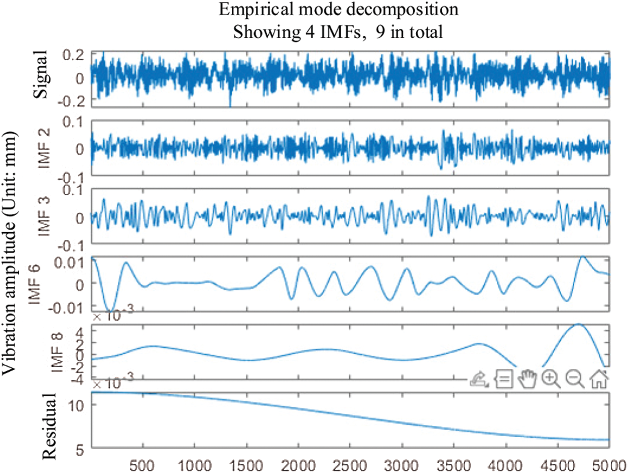
Figure 1: IMF component image of healthy signal
The envelope spectrum is shown in Fig. 2.
In Fig. 2, the theoretical vibration frequency in a healthy state is 29.95 Hz. Some other peak points can also be seen on the graph, which are noise and interference.
Analyze the signal of the bearing inner ring failure. First, according to the criterion that the kurtosis value is greater than 3, the decomposed 10 IMF components are screened. Therefore, the selected components are IMF1, IMF2, IMF4, IMF5, IMF6, IMF8. Second, draw the filtered IMF component diagram and envelope spectrum diagram. The IMF image is shown in Fig. 3.
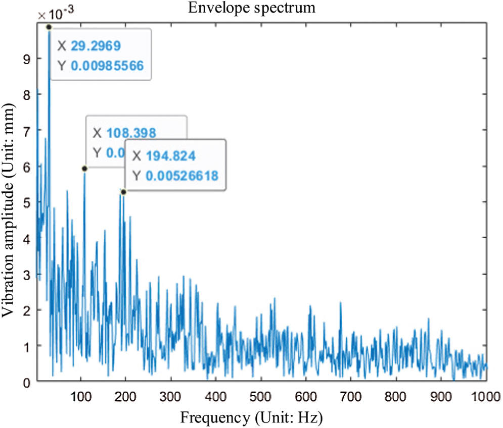
Figure 2: Envelope spectrum of healthy IMF components
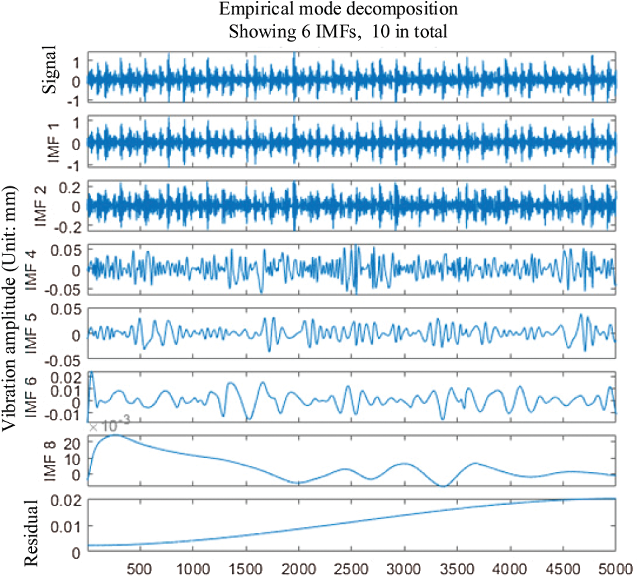
Figure 3: IMF component image of the inner ring fault state signal
The envelope spectrum is shown in Fig. 4.
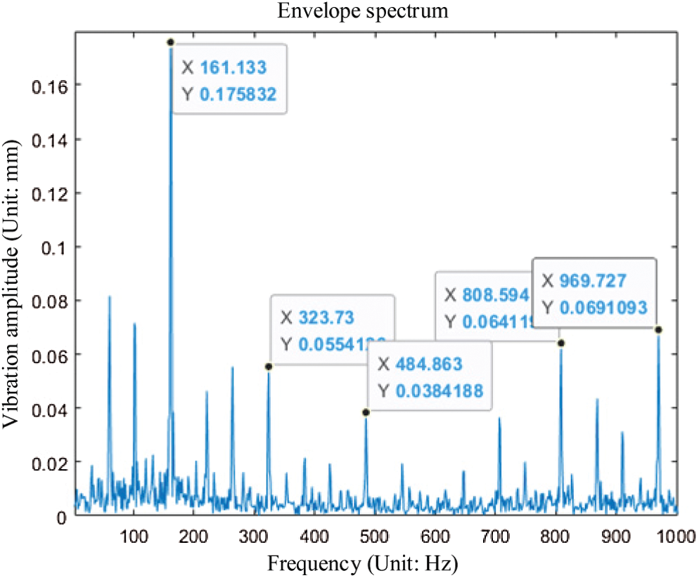
Figure 4: Inner ring fault envelope spectrum
In Fig. 4, the theoretical vibration frequency in a healthy state is 161.83 Hz. Some other peak points can also be seen on the graph, which are noise and interference.
Analyze the original signal of the bearing rolling element failure. First, according to the criterion that the kurtosis value is greater than 3, the decomposed 10 IMF components are screened. Therefore, the selected components are IMF2, IMF3. Second, draw the filtered IMF component diagram and envelope spectrum diagram. The IMF image is shown in Fig. 5.
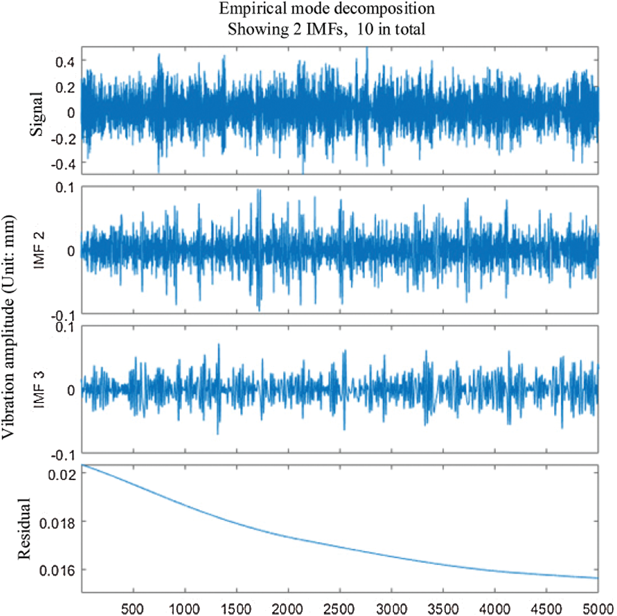
Figure 5: IMF component of rolling element fault state signal
The envelope spectrum is shown in Fig. 6.
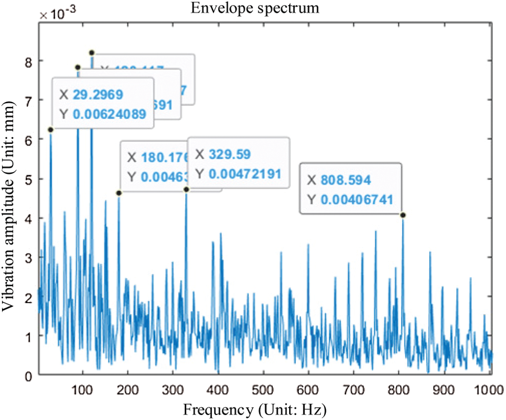
Figure 6: Rolling element fault envelope spectrum
In Fig. 6, it is obvious that the healthy vibration frequency and its frequency multiplier can be seen, but the vibration frequency of the rolling element failure is not found. Therefore, it cannot be thoroughly analyzed and determined to be the rolling element failure.
Analyze the original signal of the bearing outer ring failure. First, according to the criterion that the kurtosis value is greater than 3, the decomposed 10 IMF components are screened. Therefore, the selected components are IMF1∼IMF9. Second, draw the filtered IMF component diagram and envelope spectrum diagram. The IMF image is shown in Fig. 7.
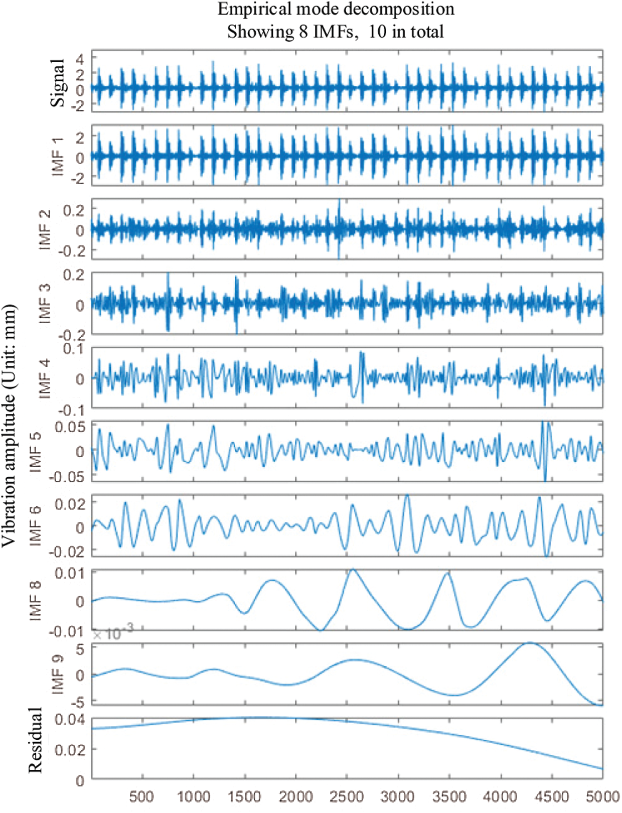
Figure 7: The kurtosis value of each IMF component
The envelope spectrum is shown in Fig. 8.
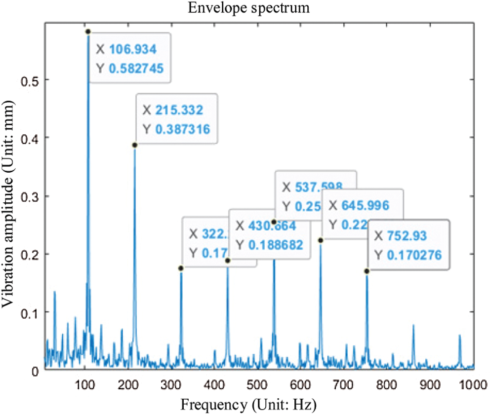
Figure 8: Outer ring fault envelope spectrum
In Fig. 8, it can be found that the fault vibration frequency of the envelope spectrum image of this state is the most noticeable image of the fault vibration frequency. The noise and interference also are less.
4 Fault Analysis of Rolling Bearing Based on EMD-KNN Method
The work of the previous chapter mainly focused on feature extraction, fault analysis, and diagnosis for a single signal. After EMD processing the data, this paper uses the envelope spectrum to analyze the failure of rolling bearings. Although the analysis results of the health status and the failure status of the outer ring are very obvious, the analysis results of the failure status of the rolling elements are disturbed. In the work of this chapter, the input signal is a complex mixed signal. The neural network classifier is added to find the frequency characteristics of each state from the complex signal. In this way, the correctness of the fault analysis and diagnosis can be ensured.
First, preprocess the original data and perform the same preliminary work as the previous chapter to obtain the IMF components selected by the kurtosis criterion. Second, superimpose the IMF components to calculate the time-frequency domain parameters of the superimposed signal. Third, normalize the computed data. Fourth, select four classifiers to train and classify the data. Finally, after comparison, a suitable classifier can be selected.
4.1 Signal Feature Extraction in Time-Frequency Domain
Since the previous work is similar to the previous work of Chapter 3, it will not be repeated here. The superimposed signal of the IMF component is obtained directly for calculation.
4.1.1 Signal Time Domain Characteristic Parameters
(1) Peak difference (
where:
(2) Standard deviation (
where:
(3) Kurtosis value (
where: y is given signal;
(4) Average (
where: N is the number of data points of the signal.
4.1.2 Signal Frequency Domain Characteristic Parameters
(1) Mean square frequency (
where:
(2) Root mean square frequency (
(3) Frequency variance (
where:
(4) Frequency standard deviation (
4.1.3 Calculation Results of Characteristic Parameters
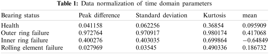
The calculated data is the superposition of the IMF components selected by the kurtosis criterion in Chapter 3. First, select one hundred thousand of the data points. Second, call the reshape function. Third, turn the hundred thousand data into a 5000 × 20 matrix. The matrix represents each state divided into 20 sets, and each set of data has 5000 data points. When repeating the above steps, four 5000 × 20 matrices of four states are obtained. According to Eqs. (18)–(25), calculated in MATLAB software, eight time-frequency domain characteristic parameters will form a 20 × 1 matrix. This matrix is the parameter value of each group of data in each state.
Since each feature parameter has its dimension, it is not convenient to directly join the neural network. Therefore, this article uses the method of data normalization to normalize the data. The data are normalized as shown in Table 1.
4.2 Failure Analysis and Simulation of Rolling Bearings
4.2.1 Vibration Signal Analysis Method of Rolling Bearing
Naive Bayes (NB) [28]: This method is one of the classic learning algorithms. The idea of this algorithm is based on probability prediction. Its theoretical basis is conditional probability, Set of Word (SOW) model, and Bag of Words (BOW) model [29]. The core of the method is Bayes’ rule, and the key of Bayes’ rule is conditional probability. SOW model is to count whether a certain term appears in the document in a given document. BOW model is used to calculate the frequency of a certain term in a given document. In addition, high-frequency words and stop words with very low importance need to be eliminated. Therefore, The BOW model is more accurate and effective.
K-Nearest Neighbor (KNN) [30]: This algorithm has three basic elements: K value, distance measurement, and classification decision rules. If the K value is too small, the accuracy will be reduced. However, if it is too large, irrelevant data will be included, and the classification effect will be reduced. Therefore, a reasonable K value should be selected. The greater the number of variables, the worse the ability to distinguish Euclidean distance; the greater the range of the variable, the variable will play a leading role in the distance calculation. Therefore, the variables must be standardized first. The classification decision rules generally choose the weighted voting method.
Discriminant Analysis Classifier (DAC) [31]: This method is an adaptive segmentation algorithm based on multi-feature discriminant analysis. It is generally used for image segmentation problems. In this method, in order to learn a linear transformation matrix, each input high-dimensional sample is converted into a low-dimensional vector through a linear transformation.
This paper will divide the raw signal data of each of the four vibration states of rolling bearings into 20 groups with 5000 data in each group, a total of 80 groups of data. Among the 20 sets of data in each state, 15 sets are used to train the classifiers, a total of 60 sets; the remaining 5 sets of data in each state are tested to determine the fault diagnosis accuracy and effects of several classifiers.
Training and testing are implemented in MATLAB software. Use the tic toc function for timing and accuracy calculations. The four classifiers are operated separately. Finally, the classification accuracy of the KNN neural network is 100%, which takes 0.449198 s and the Random Forest classifier (RF) neural network takes 2.161731 s. The characteristic of the K-nearest neighbor classifier is to follow the data to judge completely, and there is no specific fixed mathematical model.
In this way, using the other three classifier operations, the final result is shown in Table 2.
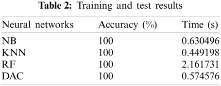
Since the test data is less and the characteristic parameters are more obvious, the accuracy of the four classifiers is 100%. However, it can be seen that the running time of each classifier is different. Among them, the longest time-consuming is RF, which takes 2.161731 s. The shortest time-consuming is KNN, which takes 0.449198 s.
On the premise of this sample of rolling bearing vibration signal data, the classification effect of the K nearest neighbor classifier is better than the other three classifiers. Therefore, the EMD-KNN method not only improves the accuracy of the typical fault diagnosis of rolling bearings but also only uses one operation to obtain the final result.
This paper takes the rolling bearing in the wind turbine generator as the research object, extracts the characteristics of its vibration signals in four different states, processes the signals based on EMD, and uses different methods for fault analysis. The research results of this paper are as follows: (1) The experimental results show that relative to directly observing the original signal, the signal characteristics after processing are more obvious, and it is easier to perform fault analysis and diagnosis. (2) Based on the EMD processed data, the time-frequency domain feature extraction is performed. Four neural network classifiers are added to obtain a more efficient and fast fault analysis method. It shows that fault analysis and diagnosis can be carried out more quickly and conveniently after joining the neural network.
Funding Statement: The support from the Guangdong Basic and Applied Basic Research Foundation (Grant No. 2021A1515012070), the Sichuan Science and Technology Program (Grant Nos. 2021YFS0336 and 2019YJ0712), the Fundamental Research Funds for the Central Universities (Grant No. ZYGX2019J035), and the Sichuan Science and Technology Innovation Seedling Project Funding Project (Grant No. 2020023) are gratefully acknowledged.
Conflicts of Interest: The authors declare that they have no conflicts of interest to report regarding the present study.
1. Liu, Z., Zhang, L. (2020). A review of failure modes, condition monitoring and fault diagnosis methods for large-scale wind turbine bearings. Measurement, 149, 107002. DOI 10.1016/j.measurement.2019.107002. [Google Scholar] [CrossRef]
2. Ilkılıç, C., Aydın, H., Behçet, R. (2011). The current status of wind energy in Turkey and in the world. Energy Policy, 39, 961–967. DOI 10.1016/j.enpol.2010.11.021. [Google Scholar] [CrossRef]
3. Liu, S., Jiang, H., Wu, Z., Li, X. (2022). Data synthesis using deep feature enhanced generative adversarial networks for rolling bearing imbalanced fault diagnosis. Mechanical Systems and Signal Processing, 163, 108139. DOI 10.1016/j.ymssp.2021.108139. [Google Scholar] [CrossRef]
4. Tan, J., Fu, W., Wang, K., Xue, X., Hu, W. et al. (2019). Fault diagnosis for rolling bearing based on semi-supervised clustering and support vector data description with adaptive parameter optimization and improved decision strategy. Applied Sciences, 9, 1676. DOI 10.3390/app9081676. [Google Scholar] [CrossRef]
5. Tao, H., Wang, P., Chen, Y., Stojanovic, V., Yang, H. (2020). An unsupervised fault diagnosis method for rolling bearing using STFT and generative neural networks. Journal of the Franklin Institute, 357, 7286–7307. DOI 10.1016/j.jfranklin.2020.04.024. [Google Scholar] [CrossRef]
6. Huo, Z., Zhang, Y., Shu, L., Gallimore, M. (2019). A new bearing fault diagnosis method based on fine-to-coarse multiscale permutation entropy, laplacian score and SVM. IEEE Access, 7, 17050–17066. DOI 10.1109/ACCESS.2019.2893497. [Google Scholar] [CrossRef]
7. Zhang, C., Yao, W., Deng, W. (2020). Fault diagnosis for rolling bearings using optimized variational mode decomposition and resonance demodulation. Entropy, 22, 739. DOI 10.3390/e22070739. [Google Scholar] [CrossRef]
8. McFadden, P. D., Smith, J. D. (1984). Vibration monitoring of rolling element bearings by the high-frequency resonance technique–A review. Tribology International, 17, 3–10. DOI 10.1016/0301-679X(84)90076-8. [Google Scholar] [CrossRef]
9. Liu, F., Gao, J., Liu, H. (2020). The feature extraction and diagnosis of rolling bearing based on CEEMD and LDWPSO-PNN. IEEE Access, 8, 19810–19819. DOI 10.1109/Access.6287639. [Google Scholar] [CrossRef]
10. Li, X., Ma, Z., Kang, D., Li, X. (2020). Fault diagnosis for rolling bearing based on VMD-fRFT. Measurement, 155, 107554. DOI 10.1016/j.measurement.2020.107554. [Google Scholar] [CrossRef]
11. Chen, Y., Zhang, T., Luo, Z., Sun, K. (2019). A novel rolling bearing fault diagnosis and severity analysis method. Applied Sciences, 9, 2356. DOI 10.3390/app9112356. [Google Scholar] [CrossRef]
12. Liu, X., Liu, X., Zhou, Z., Hu, L. (2021). An efficient multi-objective optimization method based on the adaptive approximation model of the radial basis function. Structural and Multidisciplinary Optimization, 63, 1385–1403. DOI 10.1007/s00158-020-02766-2. [Google Scholar] [CrossRef]
13. Liu, X., Wang, X., Xie, J., Li, B. (2020). Construction of probability box model based on maximum entropy principle and corresponding hybrid reliability analysis approach. Structural and Multidisciplinary Optimization, 61(2), 599–617. DOI 10.1007/s00158-019-02382-9. [Google Scholar] [CrossRef]
14. Zhou, Z., Chen, S., Liu, X. (2020). The design of linear magnetic negative stiffness element for engineering application using rectangular permanent magnets. Journal of Magnetics, 25(2), 172–180. DOI 10.4283/JMAG.2020.25.2.172. [Google Scholar] [CrossRef]
15. Zhu, S. P., Keshtegar, B., Trung, N. T., Yaseen, Z. M., Bui, D. T. (2021). Reliability-based structural design optimization: Hybridized conjugate mean value approach. Engineering with Computers, 37(1), 381–394. DOI 10.1007/s00366-019-00829-7. [Google Scholar] [CrossRef]
16. Zhu, S. P., Keshtegar, B., Bagheri, M., Hao, P., Trung, N. T. (2020). Novel hybrid robust method for uncertain reliability analysis using finite conjugate map. Computer Methods in Applied Mechanics and Engineering, 371, 113309. DOI 10.1016/j.cma.2020.113309. [Google Scholar] [CrossRef]
17. Zhu, S. P., Keshtegar, B., Tian, K., Trung, N. T. (2021). Optimization of load-carrying hierarchical stiffened shells: Comparative survey and applications of six hybrid heuristic models. Archives of Computational Methods in Engineering, 28, 4153–4166. DOI 10.1007/s11831-021-09528-3. [Google Scholar] [CrossRef]
18. Su, X., Li, L., Qian, H., Mahadevan, S., Deng, Y. (2019). A new rule to combine dependent bodies of evidence. Soft Computing, 23(20), 9793–9799. DOI 10.1007/s00500-019-03804-y. [Google Scholar] [CrossRef]
19. Su, X., Li, L., Shi, F., Qian, H. (2018). Research on the fusion of dependent evidence based on mutual information. IEEE Access, 6, 71839–71845. DOI 10.1109/Access.6287639. [Google Scholar] [CrossRef]
20. Li, Y. H., Sheng, Z., Zhi, P., Li, D. (2019). Multi-objective optimization design of anti-rolling torsion bar based on modified NSGA-III algorithm. International Journal of Structural Integrity. 12(1), 17–30. DOI 10.1108/IJSI-03-2019-0018. [Google Scholar] [CrossRef]
21. Nasir, N. N. M., Singh, S., Abdullah, S., Haris, S. M. (2019). Accelerating the fatigue analysis based on strain signal using hilbert–Huang transform. International Journal of Structural Integrity. 10(1), 118–132. DOI 10.1108/IJSI-06-2018-0032. [Google Scholar] [CrossRef]
22. Theotokoglou, E. E., Balokas, G., Savvaki, E. K. (2019). Linear and nonlinear buckling analysis for the material design optimization of wind turbine blades. International Journal of Structural Integrity. 10(6), 749–765. DOI 10.1108/IJSI-02-2018-0011. [Google Scholar] [CrossRef]
23. Yang, J., Huang, D., Zhou, D., Liu, H. (2020). Optimal IMF selection and unknown fault feature extraction for rolling bearings with different defect modes. Measurement, 157, 107660. DOI 10.1016/j.measurement.2020.107660. [Google Scholar] [CrossRef]
24. Huang, N. E., Shen, Z., Long, S. R., Wu, M. C., Shih, H. H. et al. (1998). The empirical mode decomposition and the hilbert spectrum for nonlinear and non-stationary time series analysis. Proceedings of the Royal Society of London. Series A: Mathematical, Physical and Engineering Sciences, 454(1971), 903–995. DOI 10.1098/rspa.1998.0193. [Google Scholar] [CrossRef]
25. Zhao, J., Zhang, Y., Chen, Q. (2020). Rolling bearing fault feature extraction based on adaptive tunable Q-factor wavelet transform and spectral kurtosis. Shock and Vibration, 2020, 1–19. DOI 10.1155/2020/8875179. [Google Scholar] [CrossRef]
26. Wan, S., Zhang, X., Dou, L. (2018). Compound fault diagnosis of bearings using an improved spectral kurtosis by MCDK. Mathematical Problems in Engineering, 2018, 1–12. DOI 10.1155/2018/6513045. [Google Scholar] [CrossRef]
27. Wang, J., Mo, Z., Zhang, H., Miao, Q. (2019). A deep learning method for bearing fault diagnosis based on time-frequency image. IEEE Access, 7, 42373–42383. DOI 10.1109/Access.6287639. [Google Scholar] [CrossRef]
28. Yu, J., Ding, B., He, Y. (2018). Rolling bearing fault diagnosis based on mean multigranulation decision-theoretic rough set and non-naive Bayesian classifier. Journal of Mechanical Science and Technology, 32(11), 5201–5211. DOI 10.1007/s12206-018-1018-7. [Google Scholar] [CrossRef]
29. Zhang, N., Wu, L., Yang, J., Guan, Y. (2018). Naive Bayes bearing fault diagnosis based on enhanced independence of data. Sensors, 18(2), 463. DOI 10.3390/s18020463. [Google Scholar] [CrossRef]
30. Wang, H., Yu, Z., Guo, L. (2020). Real-time online fault diagnosis of rolling bearings based on KNN algorithm. Journal of Physics: Conference Series, 1486(3), 032019. DOI 10.1088/1742-6596/1486/3/032019. [Google Scholar] [CrossRef]
31. Zhou, Y., Yan, S., Ren, Y., Liu, S. (2021). Rolling bearing fault diagnosis using transient-extracting transform and linear discriminant analysis. Measurement, 178, 109298. DOI 10.1016/j.measurement.2021.109298. [Google Scholar] [CrossRef]
 | This work is licensed under a Creative Commons Attribution 4.0 International License, which permits unrestricted use, distribution, and reproduction in any medium, provided the original work is properly cited. |