Computer Modeling in Engineering & Sciences

DOI: 10.32604/cmes.2022.017010

ARTICLE

Attractive Multistep Reproducing Kernel Approach for Solving Stiffness Differential Systems of Ordinary Differential Equations and Some Error Analysis

Radwan Abu-Gdairi1, Shatha Hasan2, Shrideh Al-Omari3,*, Mohammad Al-Smadi2,4 and Shaher Momani4,5

1Department of Mathematics, Faculty of Science, Zarqa University, Zarqa, 13132, Jordan
2Department of Applied Science, Ajloun College, Al-Balqa Applied University, Ajloun, 26816, Jordan
3Department of Physics and Basic Sciences, Faculty of Engineering Technology, Al-Balqa Applied University, Amman, 11134, Jordan
4Nonlinear Dynamics Research Center (NDRC), Ajman University, Ajman, 20550, United Arab Emirates
5Department of Mathematics, Faculty of Science, The University of Jordan, Amman, 11942, Jordan
*Corresponding Author: Shrideh Al-Omari. Email: shridehalomari@bau.edu.jo
Received: 19 April 2021; Accepted: 27 July 2021

1  Introduction

During studying and modeling many basic physical phenomena, such as chemical kinematics, aerodynamics, electrical circuits, ballistics, control models, and missile guidance, a type of differential equations appears that is difficult to solve through traditional numerical procedures, called differential stiffness system, which was first highlighted in the work of Curtiss and Hirschfelder [1–6]. Mathematical stiffness models reflect the different growth rates and various dynamic processes of the considered physical systems. It arises when some of the solution components decay much more rapidly than other components because they contain the term e−λt, λ>0. Anyhow, in the last few years, several analytical methods have been exploited to give approximate solutions for ordinary differential stiff systems and physical models, including residual power series method, homotopy perturbation method, multistep second derivative method, variational iteration method, differential transform method, and block method [7–16]. Among the effective numerical methods that used to handle several types of ordinary differential equations is the reproducing kernel Hilbert space (RKHS) method. In this direction, to see more information, definitions, kinds of operators, and applications of RKHS method in solving differential and integrodifferential equations of different types and orders, the reader is asked to refer to [17–24]. By and large, when trying to apply numerical and analytical methods to solve stiff system, it fails. Indeed, the approximate solutions are valid only for a very small interval with slowly convergent as well as completely diverge in a longer interval. More specifically, consider the following stiff system:

y′(t)=15x(t)−y(t)−15e−t, (1)

subject to the initial conditions

x(0)=y(0)=1,t∈[0,5]. (2)

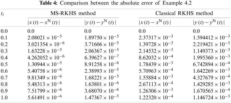
By classical RKHS method to solve this system with 100 nodes, the numerical results will be achieved under the rapid increase of the error as shown in Fig. 1. Simultaneously, increasing the number of nodes leads to the need for large computer memory along with long operating times, and cumulative errors may also affect the accuracy of the solutions. However, to overcome such drawbacks, an advanced numerical algorithm will be formulated based on dividing any temporal interval into small subintervals and then applying the standard RKHS method on each subinterval. This technique is called a multi-step reproducing Hilbert space (MS-RKHS) method. It is worth noting here that there are advanced methods in the literature to address many different engineering and physical problems, for more detail we refer to [25–30] and references therein.

Figure 1: (a) Exact (--) and classic RKHS approximate (---) solutions of system (1), (2); (b) Absolute error

By and large, there are no conventional analytical or semi-approximate methods that produce precise approximate or closed-form solutions for stiff differential systems. Therefore, there has become an urgent need for effective numerical algorithms to find accurate solutions for such models especially for large periods of time. This gives us the incentive, in this work, to explore effective accurate solutions [31–39]. Motivated by the previous discussion, our study aims to design a novel iterative algorithm to generate an analytical solution to stiff models of ordinary differential equations over a large duration through the use of a multi-step technique. To begin with, two reproducing kernel functions are established to generate a complete orthonormal basis in the Hilbert space. Based on reproducing kernel property, linear, bounded, and invertible differential operator is defined to create an analytical solution of the proposed model over a dense partition of the time period. In this direction, the approximate solution converges uniformly to the analytical solution. Error analysis is discussed as well. Lastly, some numerical examples are presented to illustrate the reliability and efficiency of the suggested multi-step approach. This paper is organized in five sections including the introduction. In Section 2, a brief description of the RKHS method is given. In Section 3, the MS-RKHS method is presented. In Section 4, several examples are given. Finally, a short conclusion is presented in Section 5.

2  Reproducing Kernel Hilbert Space Method

A reproducing kernel space is a Hilbert space H of functions defined on an abstract set X so that for each x∈X, the evaluation functional for x,δx(f)=f(x),f∈H, is continuous on H. The Riesz representation theorem gives a unique function K:X×X→C such that:

1.    ∀x∈X,K(.,x)∈H,

2.    ⟨f,K(.,x)⟩=f(x) for all x∈X and for all f∈H,

where K is the reproducing kernel function of H.

The reproducing kernel function possesses many nice properties, including it being unique, positive definite, conjugate symmetric. For the theory and applications of RKHS, we refer to [40–45].

Definition 2.1 [46]: The function space W21[a,b] is defined as

The inner product for u,v∈W21[a,b] is given by ⟨u,v⟩W21=u(a)v(a)+∫abu′(t)v′(t)dt and the norm of u is ‖u‖W21=⟨u(t),u(t)⟩W21.

Theorem 1.1 [46]: The space W21[a,b] is a complete RKHS of the reproducing kernel function Gt(s) so that Gt(s)={ 1−a+t, s≤t,1−a+s, s>t.

Definition 2.2 [47]: The function space W22[a,b] is defined by

with inner product for u,v∈W22[a,b] given by ⟨u,v⟩W22=u′(a)v′(a)+∫abu′′(t)v′′(t)dt, and the norm of u is ‖u‖W22=⟨u(t),u(t)⟩W22.

Theorem 2.2 [47]: The space W22[a,b] is a complete RKHS with reproducing function

Hereinafter, we consider the following stiff system:

x′i(t)=fi(t,x1,x2,…,xm),t∈[a,b],i=1,2,…,m,m∈N, (3)

along with the following initial conditions (ICs)

xi(t0)=ci,t0≥0. (4)

To solve system (3)–(4) using the RKHS method, we first homogenize ICs (4) in light of the following transformation:

yi(t)=xi(t)−ci,i=1,2,3,…,m, (5)

which leads to the following system:

y′i(t)=fi(t,y1+c1,y2+c2,…,ym+cm),yi(t0)=0. (6)

Subsequently, we define the differential operator L:W22[a,b]→W21[a,b] such that Lyi(t)=y′i(t),i=1,2,…,m. Hence, the system (6) can be rewritten as follows:

Lyi(t)=fi(t,y1+c1,y2+c2,…,ym+cm),yi(t0)=0,t0≥0,i=1,2,…,m. (7)

Herein, we have to construct an orthogonal function system of the space W22[a,b]. To do this, consider the countable dense set {ti}i=1∞ of [a,b], and let φi(t)=Gti(t) and ψi(t)=L∗φi(t), where L∗ is the adjoint operator of L. In terms of the properties of the reproducing kernel Gt(.), we obtain

Next, we will use the Gram-Schmidt orthogonalization process on {ψi(t)}i=1∞ to form the orthonormal function system {ψi¯(t)}i=1∞ of W22[a,b].

Let ψi¯(t)=∑l=1iβilψl(t),i=1,2,3,…, where βil are the orthogonalization coefficients which are given by

β11=1‖ψ1‖W22, βii=1‖ψi‖W222−∑p=1i−1⟨ψi(t),ψp¯(t)⟩W222, and βil=−∑p=1i−1⟨ψi(t),ψp¯(t)⟩W22βpl‖ψi‖W2−∑p=1i−1⟨ψi(t),ψp¯(t)⟩W222, for i>l.

The following theorems give the form of the solution of system (6).

Theorem 2.3: If {ti}i=1∞ is dense on [a,b] and the solution of system (6) is unique, then it has the form yi(t)=∑i=1∞∑l=1iβilfi(tl,y1+c1,y2+c2,…,ym+cm)ψi¯(t).

The N-term approximate solution yiN(t) of system (6) is given by the finite sum:

yiN(t)=∑i=1N∑l=1iβilfi(tl,y1(tl)+c1,y2(tl)+c2,…,ym(tl)+cm)ψi¯(t). (8)

Eventually, the solution of system (3) is obtained as xiN(t)=yiN(t)+ci,i=1,2,…,m.

3  Multi-Step Reproducing Kernel Hilbert Space Method

To clarify the MS-RKHS method that used in this work to find approximate solutions of system (3), we divide the interval [a,b] into equal length subintervals [tn−1,tn],n=1,2,…,M, h=b−aM and nodes t0=a,tn=a+nh. Thus, to construct the approximate solution of system (3), we first apply the standard RKHS method to the problem:

to get the approximate solution:

x1iN(t)=∑i=1N∑l=1iβ1ilfi(tl,x11(tl),x12(tl),…,x1m(tl))ψ1i¯(t)+ci. (9)

Second, we apply the standard RKHS method again to the problem:

to get the approximate solution:

x2iN(t)=∑i=1N∑l=1iβ2ilfi(tl,x21(tl),x22(tl),…,x2m(tl))ψ2i¯(t)+x1iN(t1). (10)

Continuing this process at each subinterval and applying the standard RKHS method to the problems:

to get the approximate solutions:

So, the solution of system (3) using the MS-RKHS method is given by

xniN(t)={x1iN(t),t∈[a,t1],x2iN(t),t∈[t1,t2],⋮⋮xMiN(t),t∈[tM−1,b]. (11)

4  Numerical Examples

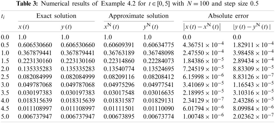
In this section, we will apply the MS-RKHS method described in Section 3 to solve some linear and nonlinear examples of stiff systems. In each example, we compare the exact solution with the approximate one when N = 100. The results are given in tables and graphs. Computations will be performed via Mathematica 10.0 software package.

Example 4.1: Consider the following homogeneous linear stiff system:

y′(t)=−x(t)−97y(t), (12)

subject to the initial conditions x(0)=y(0)=1.

The exact solution of system (12) is x(t)=147(95e−2t−48e−96t) and y(t)=147(48e−96t−e−2t). Table 1 and Fig. 2 show the numerical results for t∈[0,1]. While, If we take t∈[0,5], then the numerical and graphical results presented in Table 2 and Fig. 3 show the efficiency of the multi-step method to solve stiff system (12).

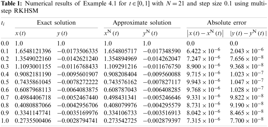
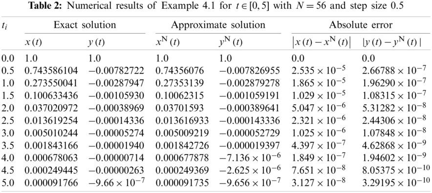
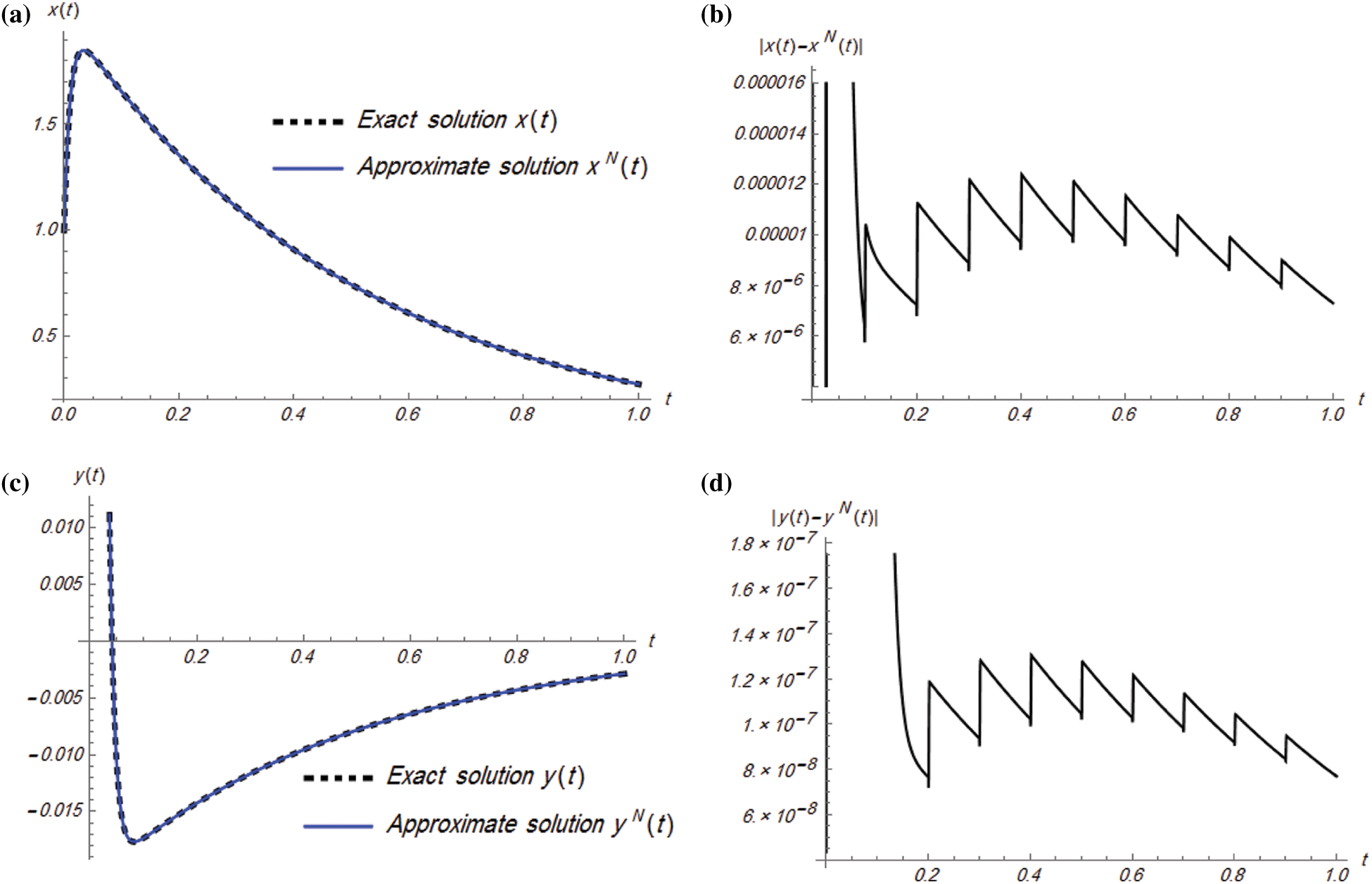
Figure 2: Plots of exact and approximate solutions and absolute error of Example 4.1 for t∈[0,1] with step size 0.1: (a) x(t), (b) |x(t)−xN(t)|, (c) y(t), (d) |y(t)−yN(t)|

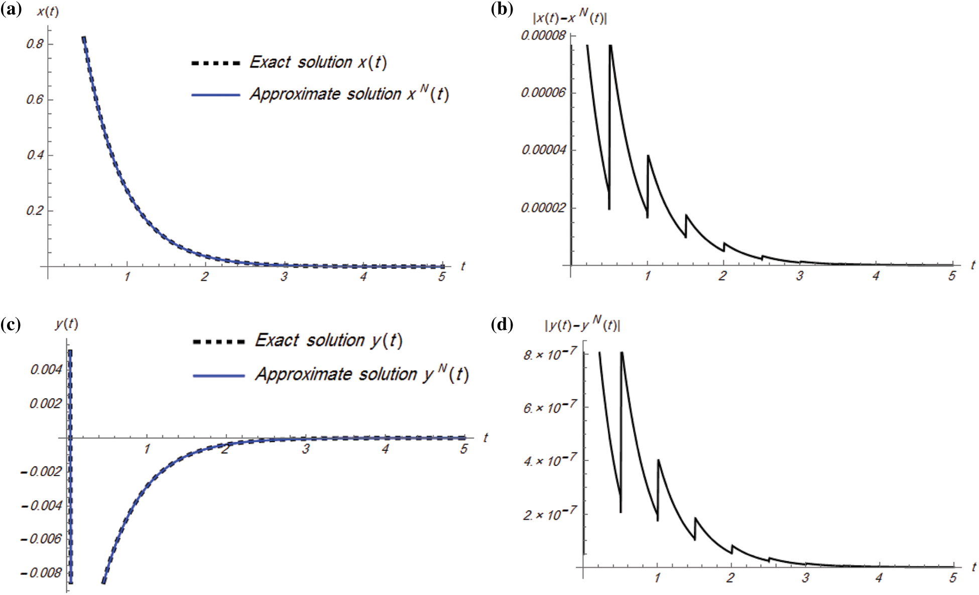
Figure 3: Plots of exact and approximate solutions and absolute error of Example 4.1 for t∈[0,5] with step size 0.5: (a) x(t), (b) |x(t)−xN(t)|, (c) y(t), (d) |y(t)−yN(t)|

Example 4.2: Consider the following nonhomogeneous linear stiff system:

y′(t)=15x(t)−y(t)−15e−t, (13)

subject to the initial conditions x(0)=y(0)=1.

The exact solution of system (13) is x(t)=y(t)=e−t. Numerical and graphical results of system (13) for t∈[0,5] with step size 0.5 are shown in Table 3 and Fig. 4. Furthermore, a comparison between the absolute error results is provided in Table 4 by using the classical RKHS method and MS-RKHS for t∈[0,1] with step size 0.1 and N=100 to illustrate the superiority of the proposed multi-step approach.

Example 4.3: Consider the following nonlinear stiff system:

y′(t)=x(t)−y(t)−y2(t), (14)

subject to the initial conditions x(0)=y(0)=1.

The exact solution of system (14) is x(t)=e−2t,y(t)=e−t. Herein, Table 5 and Fig. 5 show the numerical results for t∈[0,1] with step size 0.1 and N=50.

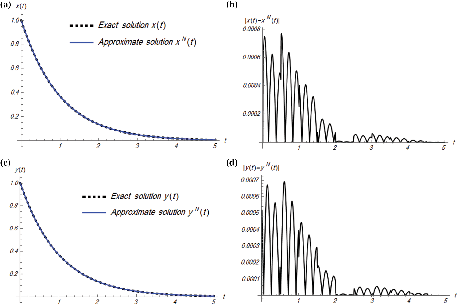
Figure 4: Plots of exact and approximate solutions and absolute error of Example 4.2 for t∈[0,5] with step size 0.5: (a) x(t), (b) |x(t)−xN(t)|, (c) y(t), (d) |y(t)−yN(t)|

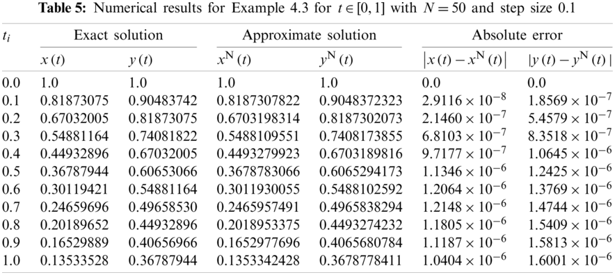
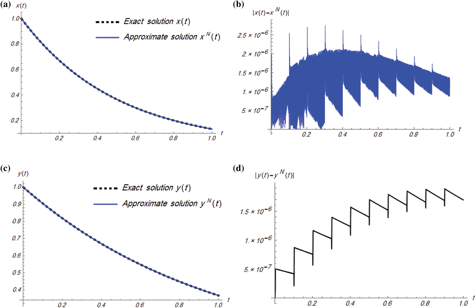
Figure 5: Plots of exact and approximate solutions and absolute error of Example 4.3 for t∈[0,1] with step size 0.1: (a) x(t), (b) |x(t)−xN(t)|, (c) y(t), (d) |y(t)−yN(t)|

Example 4.4: Consider the following stiff system:

z′(t)=20x(t)−19.75y(t)−0.25z(t), (15)

subject to the initial conditions x(0)=1,y(0)=0,z(0)=−1.

The exact solution of system (15) is given as

In the following, some numerical and graphical simulation of Example 4.4 are performed in Table 6 and Fig. 6 for t∈[0,2] with step size 0.2.

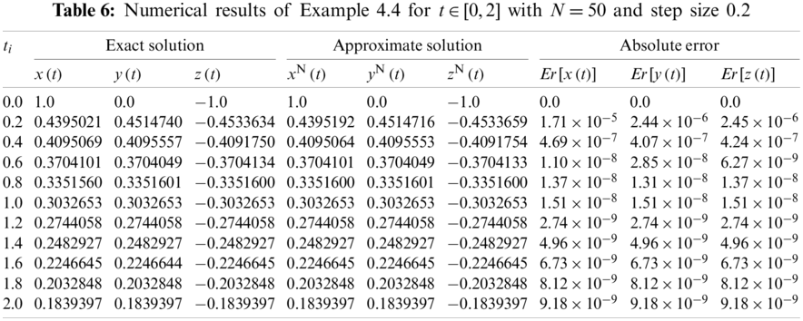
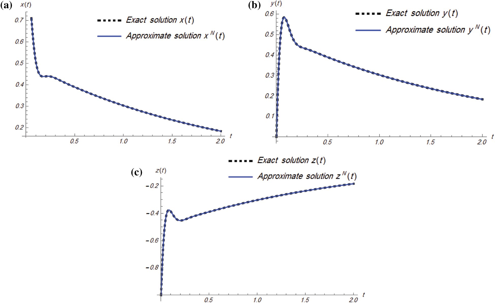
Figure 6: Plots of the exact and approximate solutions of Example 4.4 for t∈[0,2] with step size 0.2: (a) x(t), (b) y(t), and (c) z(t)

5  Conclusion

In this work, a modified multi-step algorithm, the MS-RKHS method, has been lucratively implemented based on the standard RKHS method to obtain approximate solutions of stiff systems of ordinary differential equations. Several examples of linear and non-linear stiff systems have been given to show the efficiency of the proposed method. The achieved results have been presented numerically and graphically as well. By comparing our results with the exact solutions and classical RKHS method, we observe that the MS-RKHS method yields accurate approximations. Moreover, using the MS-RKHS method, the intervals of convergence for the series solution will increase without needing large computer memory, which takes less time to give accurate numerical results. For the near future work, the presented multi-step approach will be applied for solving stiff systems of fractional and partial differential equations along with nonclassical conditions.

Acknowledgement: Authors would like to thank reviewers for their insightful comments and suggestions. The first author is grateful for the support provided by Zarqa University, Jordan.

Funding Statement: The authors received no specific funding for this study.

Conflicts of Interest: The authors declare that they have no conflicts of interest to report regarding the present study.

This work is licensed under a Creative Commons Attribution 4.0 International License, which permits unrestricted use, distribution, and reproduction in any medium, provided the original work is properly cited.