Computer Modeling in Engineering & Sciences

DOI: 10.32604/cmes.2021.016784

ARTICLE

Model Reduction by Generalized Falk Method for Efficient Field-Circuit Simulations

Dedicated to Professor Karl Stark Pister for his 95th birthday

Loc Vu-Quoc1,✉, Yuhu Zhai2 and Khai D. T. Ngo3

1,✉ Aerospace Engineering, University of Illinois at Urbana-Champaign, Illinois, 61801, USA • ✉ vql@illinois.edu
2Princeton Plasma Physics Laboratory, Princeton, New Jersey, 08542-0451, USA • yzhai@pppl.gov
3Electrical and Computer Engineering, Virginia Tech, Virginia, 24061, USA • ktn@vt.edu

Introduction

Except for very simple systems, computer simulations involving coupled field-circuit problems are hindered by the very large number of degrees of freedom involved in the discretized field problem. The evaluation of the exact natural frequencies and mode shapes for large complex systems often requires a large number of numerical operations. The direct engineering significance of this information, however, may be of limited value. For most analyses, one potentially useful approach to overcome this computational difficulty is model-order reduction, where parts of the original large-order model are replaced by models of substantially lower order, yet capable of capturing the behavior of the original subsystem with sufficient engineering accuracy.

Reduced-order models have been developed in many areas of engineering, such as circuits (e.g., [1–4]), power systems (e.g., [5–7]), electromagnetics (e.g., [8 –10]), fluid mechanics (e.g., [11–13]), nonlinear structural mechanics and earthquake engineering (e.g., [14]), nonlinear hydraulic fracturing problems (e.g., [15]), etc., to cite a few. Deep-learning artificial neural networks have been introduced to build on more traditional model-order reduction methods, such as the Proper Orthogonal Decomposition (POD)1, to increase computational efficiency [16–21].

The modal superposition method and the component-mode synthesis method for model reduction in coupled field-circuit simulations require solving a large and expensive eigenvalue problem [22]. Several alternative methods for model reduction without solving an eigenvalue problem are the well-known method in [23] and the WYD (Wilson–Yuan–Dickens) method in [24], both belonging to the general Krylov subspace methods [25, 26]. The basic idea is to find a convenient and inexpensive transformation of coordinates to simplify the equations of motion that are easier to solve. The WYD reduction method–-sometimes called the Ritz reduction method [27] or Ritz vector method [28]–-is based on the direct superposition of Ritz vectors constructed from the spatial distribution of the specified dynamic excitation; the generated Ritz vectors are thus excitation dependent. Another reduction technique called the AWE (Asymptotic Waveform Evaluation) method, a moment-matching technique based on the Padé approximation in [29], was also applied to coupled field-circuit simulation for integrated circuits (ICs) [30]. In the AWE method, the system behavior is approximated with a lower-order model, obtained from a Taylor series expansion around the Laplace transform variable s = 0. The AWE method is efficient to extract the low-frequency behavior of the circuit.

The WYD method is an efficient alternative to the classical mode superposition as discussed in [22]. In the WYD method, the solution is a direct superposition of a special class of Ritz vectors (approximated eigenvectors) generated from the spatial distribution of the excitation source; it eliminates the requirement for exact evaluation of the natural frequencies and mode shapes. It is important to note here that while the WYD method uses the excitation-dependent trial vectors to form a basis to obtain a reduced eigenvalue problem, whose solution leads to the Ritz vectors (or approximated eigenvectors), our methodology based on the Generalized Falk Method (GFM), introduced in [31], bypasses the solution of the reduced eigenvalue problem and the use of the Ritz vectors, but instead uses directly the trial vectors. To minimize the computational effort while obtaining good accuracy, the WYD method uses only Ritz vectors having large participation factors, i.e., Ritz vectors that carry a significant amount of information about the excitation.

The recursive iterative scheme used in the WYD method was shown in [31] to bear a great mathematical similarity to the Lanczos method. If the same starting vector were used in both the WYD and the Lanczos method, then the generated trial vectors from both method are very similar to each others.

Model reduction techniques based on Krylov-subspace iterations, especially the Lanczos method and the Arnoldi method2, are popular tools to tackle the large-scale time-invariant linear dynamical systems that arise in the simulation of electronic circuits, e.g., [32–40], and electromagnetics, e.g., [9, 41]. In [42] and [43], the AWE and Padé-via-Lanczos (PVL) model reduction procedures are extended to the use of electromagnetic analysis. Model reduction based on the Padé approximation may, however, produce positive poles; and is thus numerically unstable [36, 40]. The resulting reduced-order models must be post-processed to eliminate the unstable modes; such post-processing method, which must preserve the moment-matching properties, does not guarantee the elimination of unstable modes [39].

The Generalized Falk Method (GFM) proposed in [31] is shown here (Section 2.2) to be able to avoid unstable positive poles (Section 2.2.3), as the GFM can predict actually higher-order poles. We also show that the GFM is more efficient compare to other Lanczos-type methods. In [37], the block Arnoldi method is implemented via a simple congruence transformation, which guarantees the passivity and thus stability of the generated reduced-order model. Unlike the GFM introduced here, eigen decomposition is still needed, however, in the Passive Reduced-Order Interconnect Macro modeling Algorithm (PRIMA). Similar to the block Arnoldi method, the number of moments matched in PRIMA implementation is essentially the same as that for the block Arnoldi method, which is 50% of those moments matched by the block Lanczos method. The GFM applied to coupled field-circuit problems such as electrothermal simulations, on the other hand, has exactly the same order of accuracy as the Lanczos method since the resulting finite element matrices are symmetric and nonnegative. In particular, the capacitance matrix is positive definite, and thus invertible. For general circuit problems where the capacitance and conductance matrices are not symmetric, the GFM has the same order of accuracy as the Arnoldi method.

In this paper, to study the truncation effect in the proposed GFM, we first introduce the concept of participation factors for the selection of the trial vectors (Section 2.3).

To motivate, real-world applications of the electronic devices analyzed in this paper are presented in a top-down fashion, going from the big-picture system level down to the detailed component level (Section 2.4). There are many applications of semiconductors in power electronic devices used in data centers, electric vehicles, renewable energy (solar, wind, wave and tidal power). An important real-world application system is the Tesla Model S3, for which the wheels are turned by an induction motor driven by a 3-phase AC generated by a motor inverter taking as input the DC from its battery pack; see Fig. 1. At the detailed component level, the design of the Tesla motor inverter relied on IGBTs4 [44 –48].

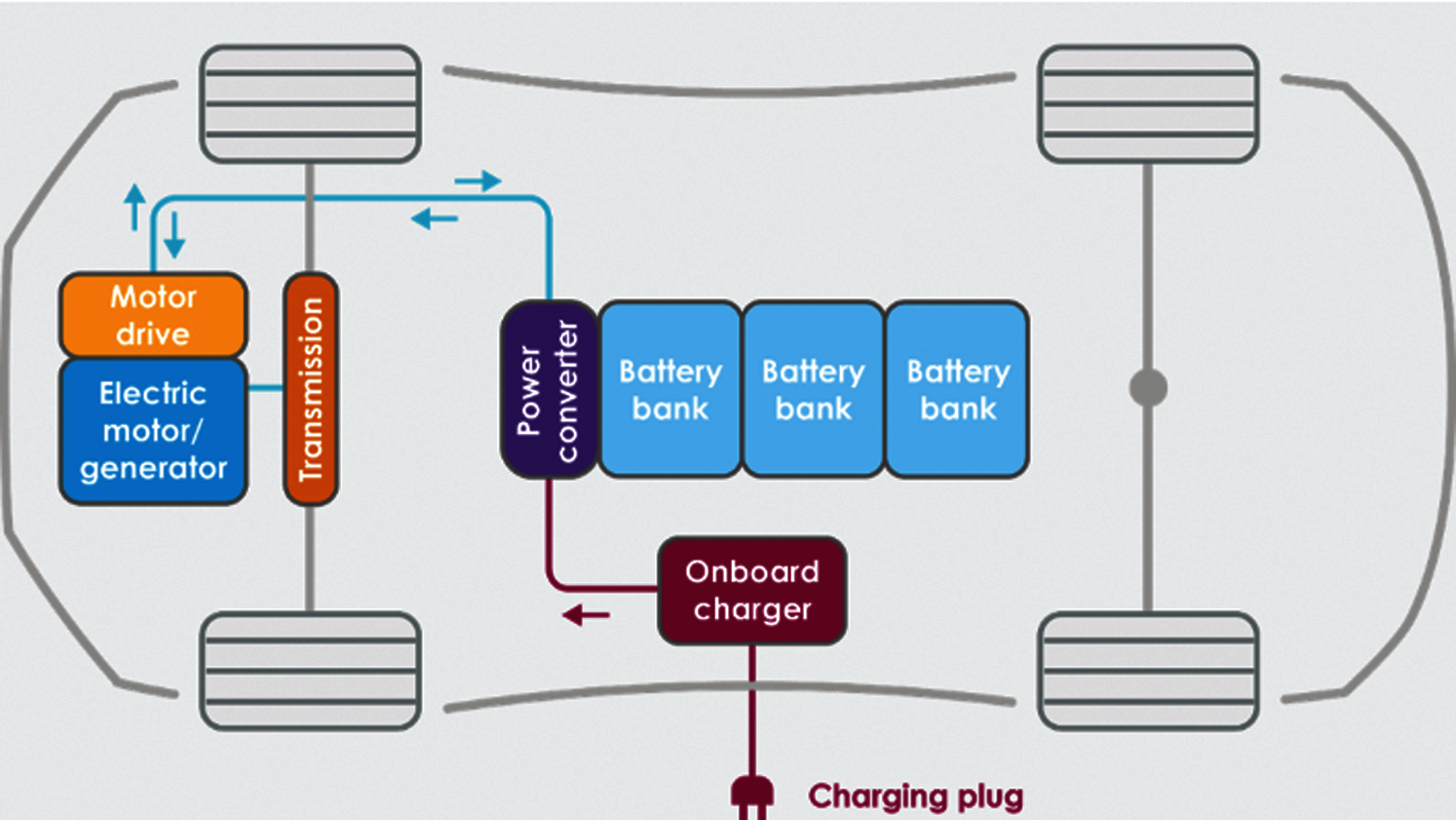
Figure 1: Battery electric vehicle schematic (Section 1). The motor drive and electric motor/generator correspond to the motor inverter and the induction motor in Footnote 3. The on-board charger is an AC-to-DC converter. The power converter transform DC to DC at different level to charge the battery and to provide DC to the motor drive (inverter). https://OpenCourseWare,TUDelft https://(CCBY-NC-SA4.0)

Remark 1.1 In writing this paper, we are mindful of the general readers, not just experts in power electronics. As a result, sufficient motivational applications and explanation for the electronic devices used here are provided. Whenever possible, permanent links to references and supporting documents on the web are provided. Wikipedia articles are provided with specific versions that are permanently fixed with no further edits, such as https://Wikipediaversion09:24,10November2020. While a link such as this https://Onlinepdf may no longer exist in the future, its https://Internetarchive version will never disappear. See also, e.g., Footnote 3.

Then we introduce two model-reduction strategies to further improve the efficiency of coupled field-circuit problems (Section 2.5), such as those encountered in electrothermal simulation or in the analysis of IC interconnects.

To illustrate the proposed model-reduction methodology, we consider a case study of coupled field-circuit problems involving electrothermal simulations; the same methodology can be applied to other coupled field-circuit problems such as IC interconnect analysis (Section 3). We next describe methods to develop simple equivalent circuit networks for the field component of the overall coupled field-circuit system (Section 3.2). We also discuss how to implement these field circuit networks into general circuit simulators (Sections 3.3, 3.4).

Numerical examples involving a full bridge converter5 using IGBTs (Section 4.2) and a Voltage Regulator Module (VRM)6 using MOSFETs7 (Section 4.3) establish the computational ease of use, accuracy, and efficiency of the present methodology; see also [51, 52]. A comparision of CPU times obtained from MATLAB and from the circuit simulator SABER is provided (Section 4.4).

Generalized Falk Method (GFM) and Model Reduction

In this paper, we present two methods to produce reduced-order models based on a combination of the proposed Generalized Falk Method (GFM) and the traditional WYD methods. These new model-reduction techniques are more stable than the traditional Lanczos method, and maintain a satisfactory accuracy. The selection of the trial vectors that form the basis for the transformation of coordinates of the original system to a reduced-order system can be based on the participation factors of these trial vectors to the dynamic response of the system. Once a reduced-order model is obtained, the dynamic response can be computed by direct numerical integration or by modal superposition method [22].

2.1 Case Study for Coupled Field-Circuit Problems

As mentioned above, to illustrate the proposed methodology, we consider electrothermal simulation as a case study of coupled field-circuit problems. The same methodology can be applied to other coupled field-circuit systems such as IC interconnects.

A typical nonlinear electrothermal coupled system can be generally expressed as

u˙=f(u,e,T),P=P(u), (1)

where u is the matrix containing the nodal voltages or currents, e the electrical input, T the temperature, and P the electrical power loss. The nonlinear electrical system is governed by the semiconductor equations (PDE’s) and circuit equations (ODE’s). The electrical power loss is originated from the heat generated inside the semiconductor devices. In practice, the electrical device needs to be treated as a distributed heat source. Here we neglect the distributed heat source, and assume the heat source is a concentrated input load to the thermal domain.

The heat diffusion problem on a domain Ω with boundary ∂Ω=Γ1∪Γ2¯ is governed by the partial differential equation

div(κgradT)=ρcp∂T∂tin Ω,(2)

and the boundary conditions on ∂Ω=Γ1∪Γ2¯:

κgradT⋅n=κ∂T∂n=PAon Γ1, (3)

κgradT⋅n=κ∂T∂n=h(Ta−T)on Γ2, (4)

and initial condition at time t = 0:

T(x,0)=Ta=27∘C,(5)

where T:Ω×R+→R is the temperature (a function of space and time), κ:Ω→R the thermal conductance, ρ:Ω→R the mass density, cp:Ω→R the specific heat, P:Γ1×R+→R the input power from boundary Γ1, A the input-power cross-section area, h the convection coefficient, n the outward normal vector to the boundary, and Ta the ambient temperature. In the above, the set of real numbers is denoted by R, with R+:={t∈R∣t≥0}, denoting the set of non-negative numbers. The domain of the heat sink is denoted by Ω⊂Rs, with s = 1, 2, 3 being the space dimension. The boundary ∂ Ω of the heat sink is decomposed into two parts: Γ1 for the input-power boundary condition Eq. (3), and Γ2 for the convective boundary condition Eq. (4). We assume in the above electrothermal coupled system that it does not include any heat source in the thermal domain Ω.

Employing a Galerkin finite element projection [53, 54] on the PDE Eq. (2), we obtain the following semi-discrete equation for the thermal system:

Cd˙+Kd=f=Ip+Ic, (6)

d(0)=d0, (7)

where C∈Rn×n, with n being the number of element nodes (or temperature unknowns/degrees of freedom or dofs), is the capacitance matrix, K∈Rn×n the conductance matrix, f∈Rn×1 the heat supply matrix, Ip the input power supply from the electrical component, Ic the heat supply coming from the convective boundary condition, and d(t)={di(t)}∈Rn×1 the column matrix of the time-dependent nodal temperatures di(t) at the finite-element (FE) node i, for i = 1,… , n. Let Ni be the shape function associated with node i, then the temperature field over the domain of the heat problem is approximated by T(x,t)≅∑i=1nNi(x)di(t). The capacitance matrix C can be realized by capacitor elements, the conductance matrix K by resistor elements, and the heat supply vector f by current sources, so that thermal effects for semiconductor devices (transistors) like an IGBT or MOSFET can be dynamically incorporated into circuit simulators with thermal connection. The global matrices C, K, f are assembled from the elemental matrices ce, ke and fe.

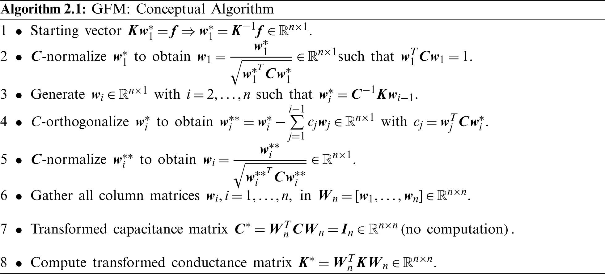
A complex mechanical system can be transformed into a simple one-dimensional mass-spring system by transforming its coordinates (degrees of freedom) using a set of linearly-independent vectors, termed trial vectors, generated by the Falk method [55]. The transformed matrices are diagonal (mass) and tridiagonal (stiffness), which upon scaling represent a one-dimensional lumped system, and have the same eigenvalues as the original system.

2.2 Generalized Falk Method (GFM)

The original Falk method suffers from the loss of orthogonality similar to that found in the original Lanczos method [56, 57], since each trial vector in the Falk method is orthogonalized with respect to only the two previously generated trial vectors. By contrast, in the GFM, each trial vector is orthogonalized with respect to all previously generated trial vectors, with the transformed tridiagonal conductance matrix constructed by formal matrix multiplication [31].

2.2.1 Conceptual Algorithm

To ensure that the generated trial vectors8 contain important information from the static response, the starting trial vector, denoted by w1∗∈Rn×1 in Line 1 of Algorithm 2.1, with n being the total number of dofs, is selected to be the static response when the spatial distribution of the dynamic excitation is applied on the system.

The traditional WYD method leads to an identity capacitance matrix C∗=WnTCWn=In∈Rn×n, with In being the identity matrix and Wn=[w1,…,wn]∈Rn×n a matrix whose columns are the trial vectors wi, but a full conductance matrix K∗=WnTKWn∈Rn×n, thus making the construction of an equivalent circuit complicated [31]. The WYD process can be truncated based on certain measure (to be discussed shortly) to obtain reduced-order models.

On the other hand, the GFM leads to an identity capacitance matrix C∗=In∈Rn×n, and a tridiagonal conductance matrix K∗∈Rn×n. The GFM can also be truncated, and the generated trial vectors can be used to construct reduced-order models. There is a trade-off in the solution of the method to use to reduce the order of a large system in a cost-effective manner, while maintaining high accuracy.

2.2.2 Implementable Algorithm

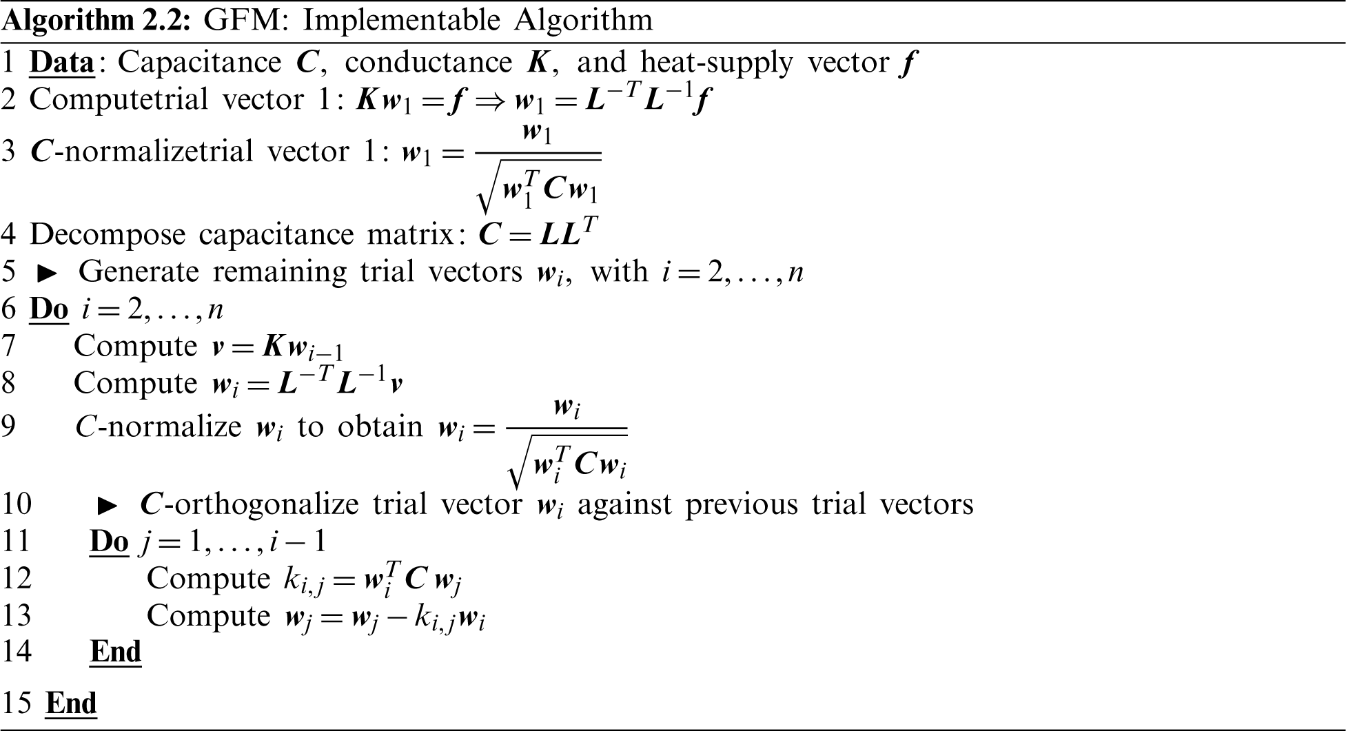
The implementation of the present GFM is presented as a pseudocode in Algorithm 2.2, with particular attention paid to the computational efficiency.

2.2.3 GFM vs. Other Methods: No Unstable Positive Poles

It is well known that direct Padé approximation that forms the basis for methods of type Lanczos does not guarantee that the reduced-order model is passive or stable [36, 37, 58]: It is possible to have unstable positive poles. By contrast, no positive pole is generated when using the GFM in circuit simulation since the higher order poles tend to be accurately predicted.

Unlike the Padé-via-Lanczos (PVL) method, Table 1 clearly shows that the GFM does not generate destabilizing positive poles in the system, which was originally stable. The PVL method was shown in [36], using the simple linear RC-circuit in Fig. 2, to possibly produce a model that was unstable even though the system was described by a symmetric, positive definite matrix. The circuit parameters are R1 = R2 = R3 = R4 = R5 = R = 1.3955 and C1 = C2 = C3 = C4 = C5 = 1. The original system capacitance matrix and conductance matrix are

K=1R[2−1000−12−1000−12−1000−12−1000−11]5×5,C=[1000001000001000001000001]5×5,(8)

and they are reduced from 5× 5 to 3× 3 in the PVL, Arnoldi, and GFM iterations. The GFM does not suffer from positive poles.

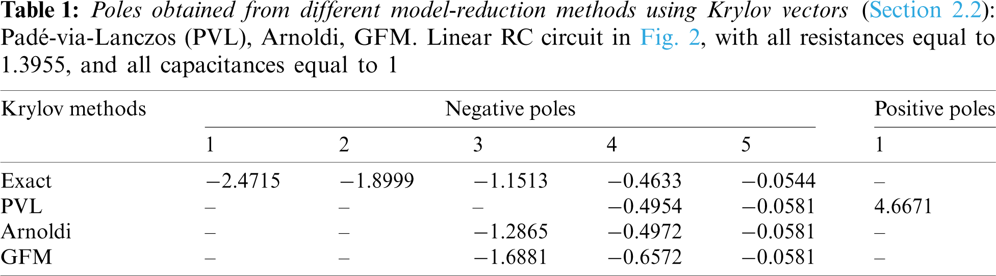
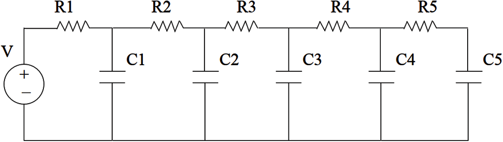
Figure 2: Simple linear RC circuit (Section 2.2). A simple linear circuit with passive elements shows that the Padé-via-Lanczos (PVL) method generates positive poles that are unstable

To detect the positive poles generated from the PVL method and the circuit resistance values R that lead to the positive poles for the circuit in Fig. 2, we swept through a set of values for the resistance R, and plot the poles generated from these three methods. Fig. 3 (left) shows clearly that the PVL method generated unstable poles, whereas the Arnoldi method (Fig. 3, right) and the GFM method (Fig. 4) did not.

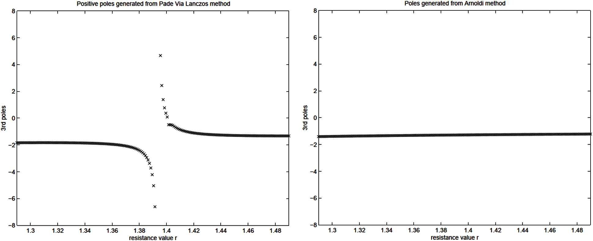
Figure 3: Simple linear circuit (Section 2.2). Values of the 3rd pole as a function of the resistance R, as generated by the Padé-via-Lanczos (PVL) method (left), and by the Arnoldi method (right) for the circuit example in Fig. 2

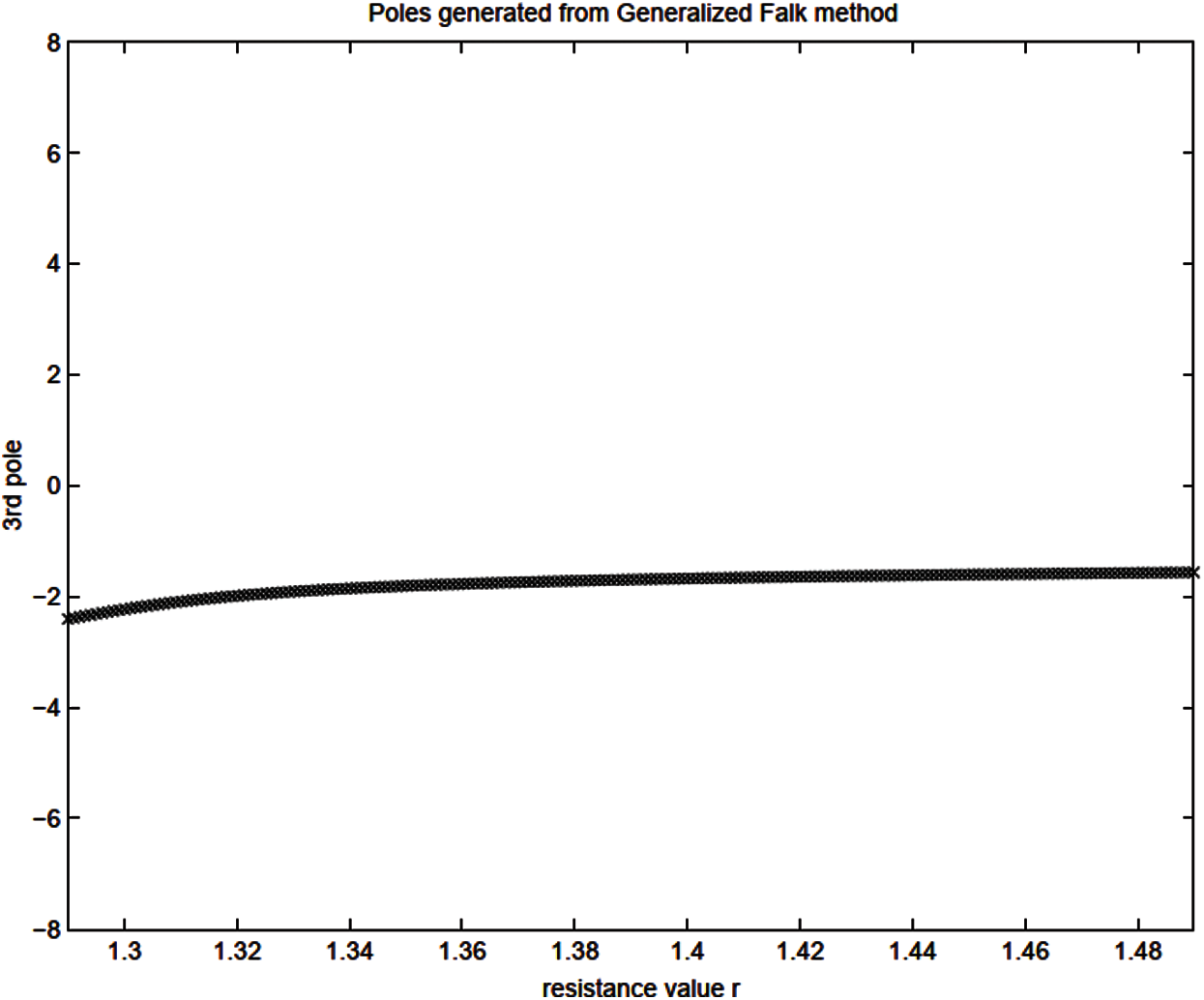
Figure 4: Simple linear RC circuit (Section 2.2). Values of the 3rd pole as a function of the resistance R, as generated by the GFM for the circuit example in Fig. 2

2.3 Participation Factors

To study the truncation effect in our proposed coordinate-transformation methods, we introduce three quantities that will serve as measures to guide the truncation of the basis of trial vectors that are used to construct reduced-order models: The projected load p, the load participation factor β, and the response participation factor α.

The superscripts L, W, F, G over these three quantities will be used to designate their association with the Lanczos, WYD, Falk, and GFM methods, respectively. Let yr(t)={y1(t),…,yr(t)}T∈Rr×1, with r ≤ n being a mnemonic for “retained” after truncation of the full basis and n the dimension of the original system (i.e., the size of the full basis, see Line 3 in Algorithm 2.1), denote the state variables in the new coordinates corresponding to the basis of the trial vectors generically written as {w1,…,wr}∈Rn×r, which can be either Lanczos vectors (L), WYD vectors (W), Falk vectors (F) or Generalized Falk vectors (G). The projected force on the basis of trial vectors is represented by pr(t)={p1,…,pr}T∈Rr×1. The load participation factor β i and the response participation factor αi are defined as

βi(t):=∥wipi(t)∥,αi(t):=∥wiyi(t)∥,(9)

respectively.

2.3.1 Lanczos Method

A projection of the matrix ODE in Eq. (6) onto the Lanczos basis vectors yields the following transformed matrix ODE [27] (see Eq. (43) in Appendix A):

Try˙r+Iryr=ZrTCK−1f=:prL,(10)

where Tr∈Rr×r, with r ≤ n and n being the size of the full basis as mentioned above, is a tridiagonal matrix consists of orthogonalization coefficients given in Eq. (39) and Eq. (41), which are similar to the coefficients cj in Algorithm 2.1, Ir∈Rr×r an identity matrix, Zr:=[w1L,…,wrL]=[z1,…,zr]∈Rn×r the matrix containing the r Lanczos trial vectors (see Appendix A), C∈Rn×n the capacitance matrix, K−1∈Rn×n the inverse of the conductance matrix, and the (truncated) projected load prL={p1L,…,prL}T∈Rr×1 with r retained components of pnL∈Rn×1 is as defined on the right-hand side. The circuit network equivalent to Eq. (10) is discussed in Section 3.2.1.

The coefficients of the full projected load matrix pnL={p1L,…,pnL}T∈Rn×1 can be interpreted as the n components of the original excitation matrix f with respect to the basis vectors that are columns of the matrix KZn∈Rn×n as follows. Before truncation, using the full basis, we can express f as

f(t)=KZnpnL(t)=∑j=1nKzjpjL(t)=K∑j=1nzjpjL(t).(11)

It can be verified that prL is indeed the excitation matrix (right-hand side) in Eq. (10) by premultiplying Eq. (11) by ZrTCK−1, with Zr=[w1L,…,wrL]=[z1,…,zr]∈Rn×r, and by using the C-orthonormality conditions for the column matrices in Zn∈Rn×n or in Zr∈Rn×r

ZnTCZn=In∈Rn×n,ZrTCZr=Ir∈Rr×r,ZrTCZn=[Ir∣0r×(n−r)]∈Rr×n.(12)

We have:

ZrTCK−1f=ZrTCK−1(KZnpnL)=(ZrTCZn)pnL=prL.(13)

Using Eq. (13) with r = n, we can also verify that

f=KZnpnL=KZn(ZnTCK−1f)=K(ZnZnTC)K−1f.(14)

Since ZnTCZn=In⇒ZnTCZnZn−1=Zn−1⇒ZnZnTC=In, thus

f=KK−1f=f.(15)

If we truncate the full basis of the n Lanczos trial vectors, and retain only r of those trial vectors, then:

f≈frL:=K∑j=1rzjpjL.(16)

The error committed in representing f by a truncated series frL is thus:

erL:=∥f−frL∥2.(17)

2.3.2 Wilson–Yuan–Dickens (WYD) Method

The reduced-order ODE in Eq. (6) for the WYD method, (Appendix B) [24], takes the form:

Iry˙r+Kr∗yr=WrTf=:prW∈Rr×1,withKr∗:=WrTKWr∈Rr×r(18)

where Wr:=[w1W,…,wrW]=[w1,…,wr]∈Rn×r contains the WYD trial vectors, with the projected load denoted by prW:=WrTf∈Rr×1 on the right-hand side of Eq. (18). With the full basis (no truncation), the excitation f can be represented in terms of the projected load pnW as follows:

f(t)=CWnpnW(t)=C∑j=1nwjpjW(t).(19)

Premultiplying Eq. (19) by WrT∈Rr×n and using the C-orthonormality conditions

WnTCWn=In∈Rn×n,WrTCWr=Ir∈Rr×r,WrTCWn=[Ir∣0r×(n−r)]∈Rr×n,(20)

We obtain:

WrTf=WrTCWnpnW=[Ir∣0r×(n−r)]pnW=prW.(21)

We can also verify that

f=CWnpnW=CWn(WnTf)=(CWnWnT)f=f.(22)

Since WnTCWn=In⇒WnTCWnWn−1=Wn−1⇒WnWnTC=In, thus

f=CWnWnTf=f.(23)

A truncated representation of the excitation matrix f using r ≤ n WYD (trial) vectors, and the resulting error on such representation can be expressed as

f≈frW:=C∑j=1rwjpjW;erW:=∥f−frW∥2.(24)

For all four methods (Lanczos, WYD, Falk, Generalized Falk), the response dr(t) in the original (physical) coordinates can be computed from the response yr(t) in the reduced trial-vector basis denoted generically here as Wr (for all four methods) as follows:

dr(t)=Wryr(t)=∑i=1rwiyi(t),with r≤n.(25)

In general, it is not necessarily true that the projected load along the first trial vector would have the highest magnitude, and then decreases along subsequent trial vectors (see Fig. 14 for example). The load participation factors βiL:=∥zipiL∥ for the Lanczos method, and βiW:=∥wipiW∥ for the WYD method (see Eq. (9)1 for the definition, which comes from Eq. (16) for the Lanczos method, and Eq. (24)1 for the WYD method) are not reliable indicators for the selection of the trial vectors to be retained for model reduction. In other words, a trial vector with a low value of load participation factor may actually play a key role in the response dr(t). This reason is why we introduce the response participation factors αiL:=∥ziyi∥ and αiW:=∥wiyi∥ (see Eq. (9)2 for the definition, which comes from Eq. (25) for the reconstructed solution), which can be used as indicators to evaluate the importance of the contribution of each trial vector to the response, and to guide the truncation of the trial-vector basis for model reduction.

2.3.3 Falk Method and Stability of Generalized Falk Method (GFM)

The GFM guarantees passivity and stability for efficient simulation of coupled field-circuit problems. We show that the GFM performs better in terms of loss of orthogonality compared to the original Falk method. Even though the Falk trial vectors and the GFM trial vectors are not identical, the final transformed systems have the same mathematical structure, i.e.,

Iry˙r+Kr∗yr=WrTf,(26)

where Wr∈Rn×r, with r ≤ n, denotes the reduced basis formed by either the Falk trial vectors or the GFM trial vectors (Line 6 in Algorithm 2.1). As a result, the transformed stiffness matrices Kn∗ (Line 8 in Algorithm 2.1), even though having the same tridiagonal topology, are also different for different method. Since we normalize the Falk trial vectors and the GFM trial vectors with respect to the capacitance matrix C, i.e., WnTCWn=In (Line 7 in Algorithm 2.1), the projected loads are similar to the case of the WYD method, i.e.,

pnF:=(WnF)Tf,pnG:=(WnG)Tf,(27)

with the excitation matrix f≡ fn decomposed as follows:

f=CWnFpnF=CWnGpnG.(28)

Similarly, the truncated representation of f, and the error committed due to the truncation are given respectively as

frF=C∑j=1rwjFpjF,frG=C∑j=1rwjGpjG. (29)

erF:=∥f−frF∥,erG:=∥f−frG∥. (30)

2.4 Applications of Discrete IGBTs and Model Participation Factors

We begin this section by providing a big picture of how discrete IGBTs are used in real-world engineering systems (Section 2.4.1), followed by an idealized model for electrothermal analysis of a discrete IGBT to deduce the desired participation factors to select modes with high participation factors for model-order reduction (Section 2.4.2).

2.4.1 Real-World Applications of IGBTs

Fig. 5 shows a single-chip power package used in power electronic circuits operating at high frequencies to achieve vastly improved performance in converters, either AC-to-DC or DC-to-DC9. The chip is a discrete IGBT embedded inside a TO-247 package, which provides mechanical support and protection, heat sink for cooling, electrical connection (through the 4 pins in Fig. 5a) and isolation. The IGBT power package with 4 pins in Fig. 5 provides much better energy efficiency during switching compared to earlier models with 3 pins, allowing for higher swithching speed, lower operating temperature, and thus better overall system performance.

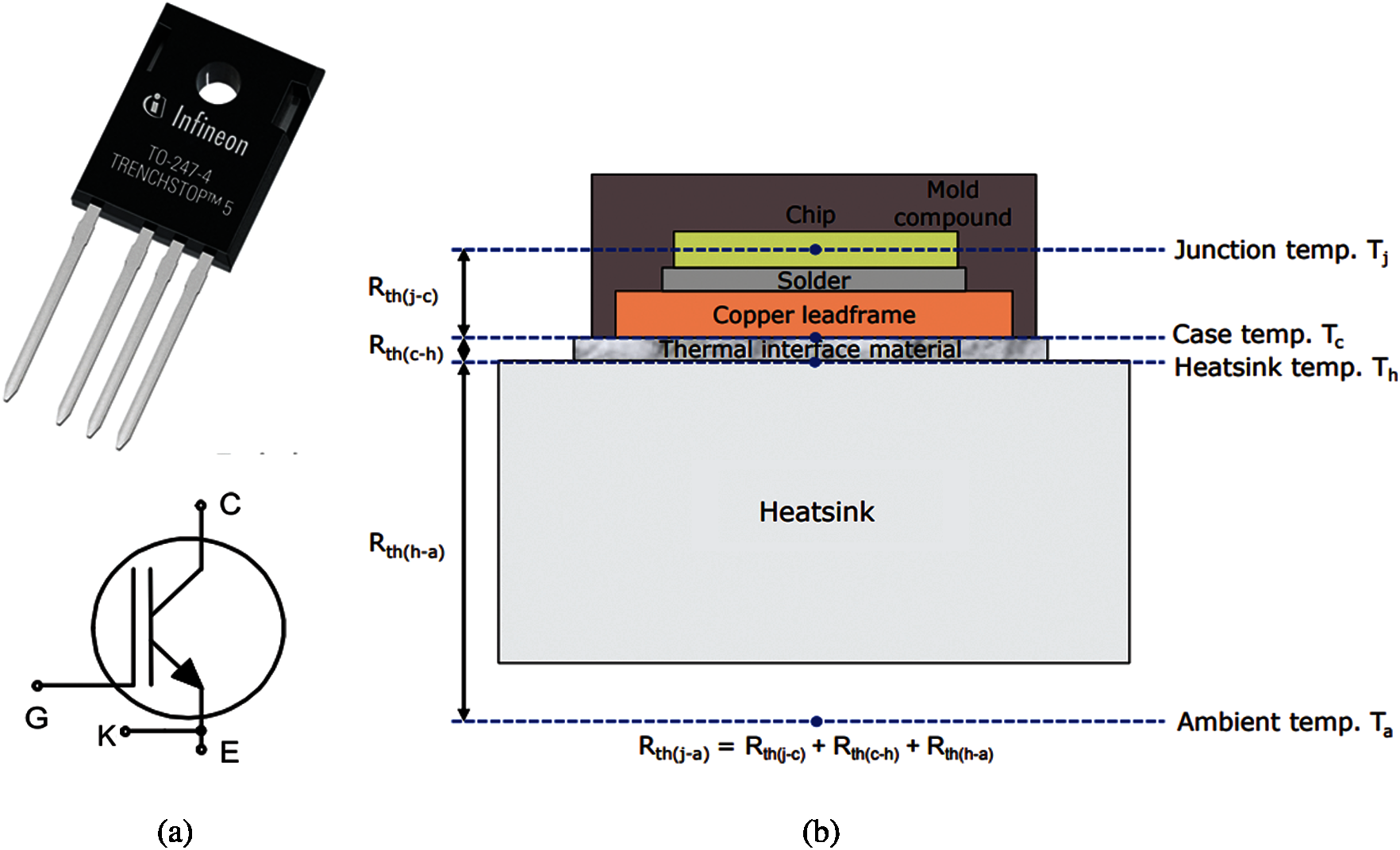
Figure 5: IGBT chip in TO-247 package (Section 2.4.1). (a) Single IGBT (Footnote 4) chip power package with through hole for mounting. Infineon (Brand name) IGZ75N65H5 (product code) device, with the TRENCHSTOP 5 IGBT chip on the Transistor-Outline (TO) 247 package with 4 pins. The dimension of the package, without the pins, is roughly W × L × H = 16 mm× 21 mm× 5 mm. (b) Material layers within the package. For the Tesla Model S electric vehicle, see Footnote 3 on the use of IGBTs with 3 pins, and Fig. 9 for the conceptual schematic of a half-bridge inverter. See Footnote 9

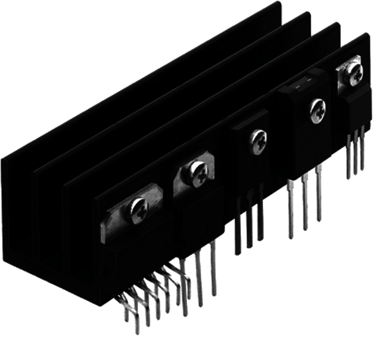
Figure 6: IGBT power packages attached to heat sink (Section 2.4.1). The middle device is a single IGBT chip with 3 pins embedded in a TO-247 package. Each IGBT power package is screwed to the heat sink via its through hole; see Figs. 5 and 7

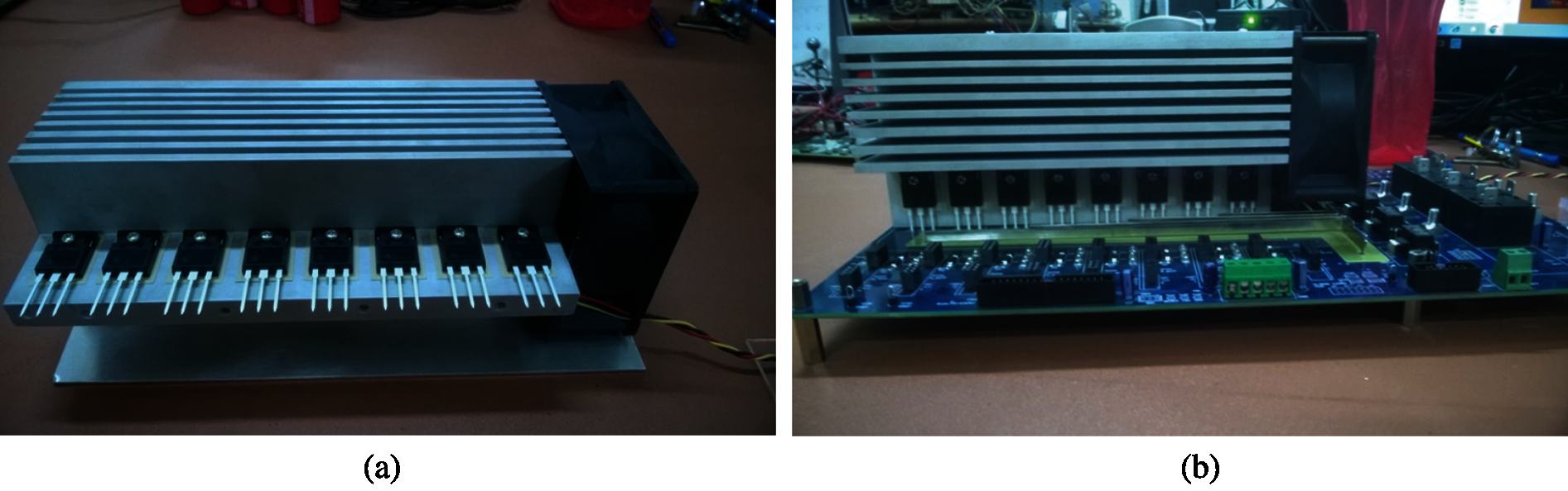
Figure 7: General purpose IGBT stack for power converter/inverter (Section 2.4.1). (a) The aluminum heat sink with 8 discrete (3-pin) IGBT power packages (Fig. 6), which are screwed on via through holes, is cooled by air pushed through by the DC fan (black) on the right end of the heat sink. (b) The assembly in (a) is then mounted on a Power Circuit Board (PCB) for a converter/inverter device; see Footnote 11 [59]. (Figures reproduced with permission of the authors)

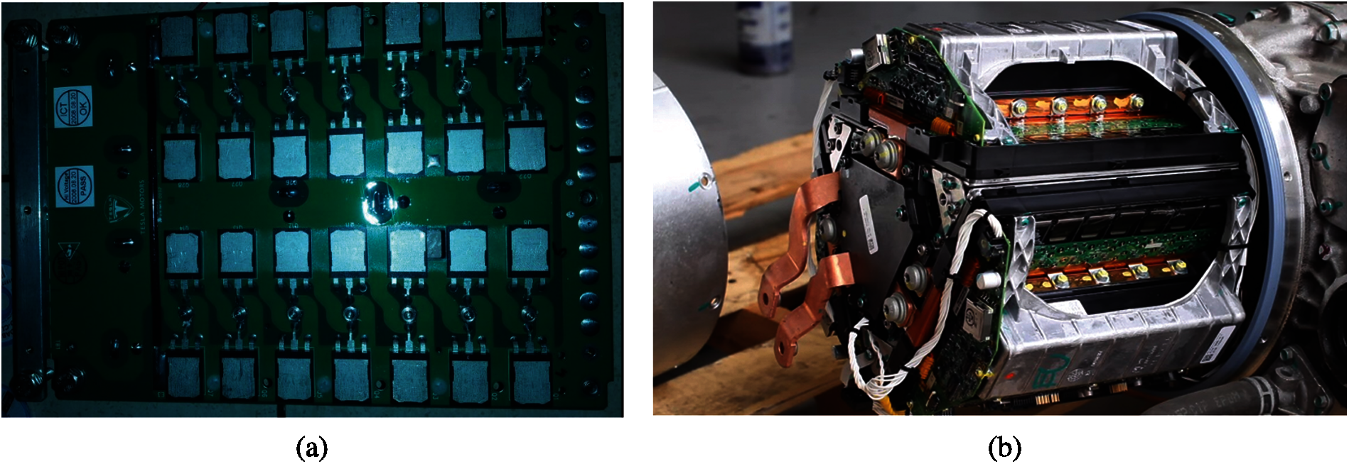
Figure 8: Tesla motor inverter (Section 2.4.1) (a) IGBT array for 2 switches, each with 14 discrete IGBTs in parallel (2 rows of 7 pairs of IGBTs). (b) Motor inverter containing an IGBT array shown in (a) for each of the 3 AC phases. See also Footnote 3 for the big picture of how these components are used in the Tesla S electric vehicle, and Fig. 9 for the generic schematic of a half-bridge inverter, having (a) as a specific implementation. https://Twinkletoesengineering.info

Fig. 6 shows 5 different types of discrete IGBT power packages mounted on a heat sink10. Fig. 7 is a General Purpose IGBT Stack (GPIS) for use in a power converter or inverter11 “rated up to 20 kVA12, and can be used in a variety of power electronic applications such as motor drives, energy storage systems, grid-tied and off-grid renewable energy systems” [59].

Fig. 8 shows a much more advanced motor inverter in the Tesla Model S electric vehicle that uses arrays of IGBTs (Fig. 8a) to convert DC from the battery pack to 3-phase AC, and thus a triangular cross section (Fig. 8b), to drive the induction motor that turns the wheels, Footnote 3.

Fig. 9 is a schematic of a half-bridge inverter in the Tesla patent [45], explaining how the IGBT array in Fig. 8a work to transform DC to the sine wave current for one of the three AC phases.

Fig. 10a shows a different geometry and material layering of the Tesla packaging from the patent application [44], compared to the packaging geometry and material layering in Fig. 5b, but the basic principles were the same.

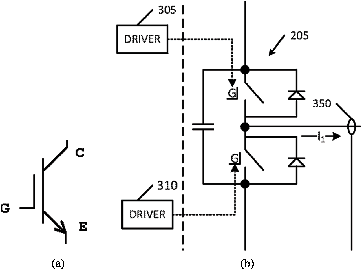
Figure 9: Tesla half-bridge inverter (Section 2.4.1). (a) Schematic of a 3-pin IGBT (Footnote 3 and Footnote 4, Gate G, Collector C, Emitter E), compared to that of a 4-pin IGBT in Fig. 5a. (b) Half-bridge inverter 205, signal from driver 305 goes into the gate G of the upper switch (representing the top two rows, each with 7 IGBTs, in Fig. 8a) to turn it on or off, likewise for driver 310 for the lower switch (bottom two rows of IGBTs in Fig. 8a), output sine wave current I1 for phase 1 of a 3-phase current, current sensor 350 to feed output current I1 back to controller system (not shown). This subfigure is part of Fig. 2 in the Tesla patent [45] (rotated by −90∘ to match the 2 switches in Fig. 8a)

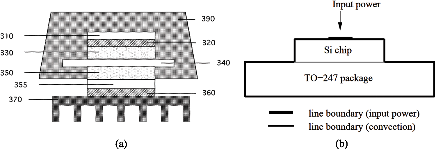
Figure 10: Tesla IGBT packaging and idealized IGBT in TO-427 package (Sections 2.4.1, 3.3, 4.1). (a) Tesla IGBT packaging. (From top to bottom layer.) An encapsulant 390 encases a portion of the device; A silicon die 310 is sintered to a semiconductor device comprising layers 330–350, below sintering layer 320. The semiconductor 340 (IGBT or MOSFET) is interspersed between two copper cladding layers 330 and 350, which lays on top of a direct bonded-copper substrate 355. The whole structure is connected to the heat sink 370 via a sintering thermally-conducting silver layer 360. Tesla inverter US patent application [44]. Fig. 5b for TO-247 packaging. (b) Coupled transistor-thermal model. IGBT chip on heat sink, compared to Figs. 5b and (a), used for electrothermal analysis and proof-of-concept for GFM. See also Fig. 29 in Section 3.3 on SABER implementation

2.4.2 Participation Factors of IGBT Electrothermal Model

We use here an idealized 2-D thermal model problem shown in Fig. 10b to illustrate the properties of the projected load pi, the load participation factor β i, and the response participation factor αi for each of the four methods discussed in the previous section: Lanczos (Figs. 11–13), WYD (Figs. 14–16), Falk (Figs. 17–19), and GFM (Figs. 20–22). The finite-element (FE) discrete model has 368 triangular elements and 215 nodes.

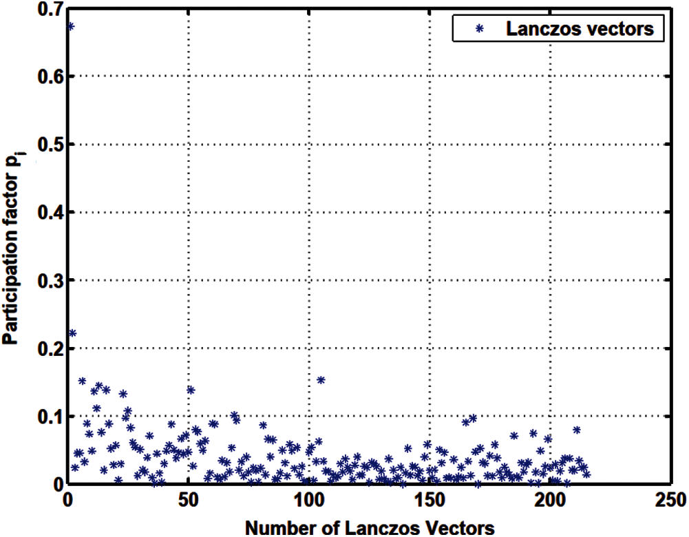
Figure 11: Projected load piL vs. Lanczos vector number (Section 2.4.2)

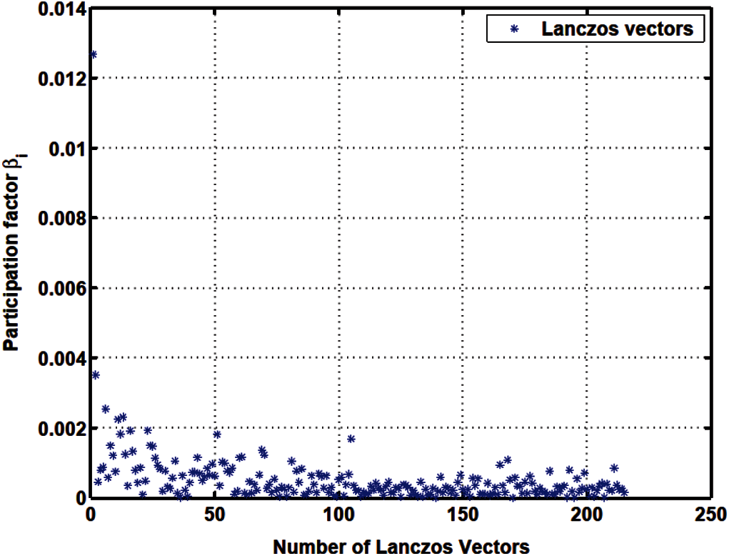
Figure 12: Load participation factor βiL vs. Lanczos vector number (Section 2.4.2)

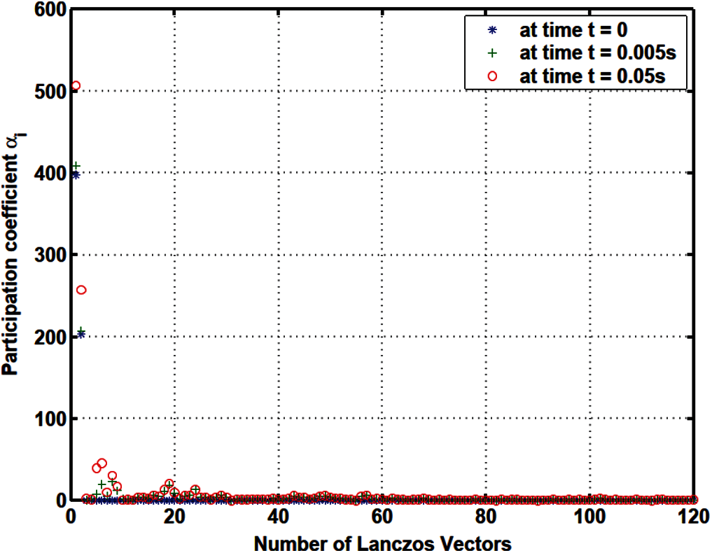
Figure 13: Response participation factor αiL vs. Lanczos vector number (Section 2.4.2): Only first 120 trial vectors among 215 trial vectors are shown

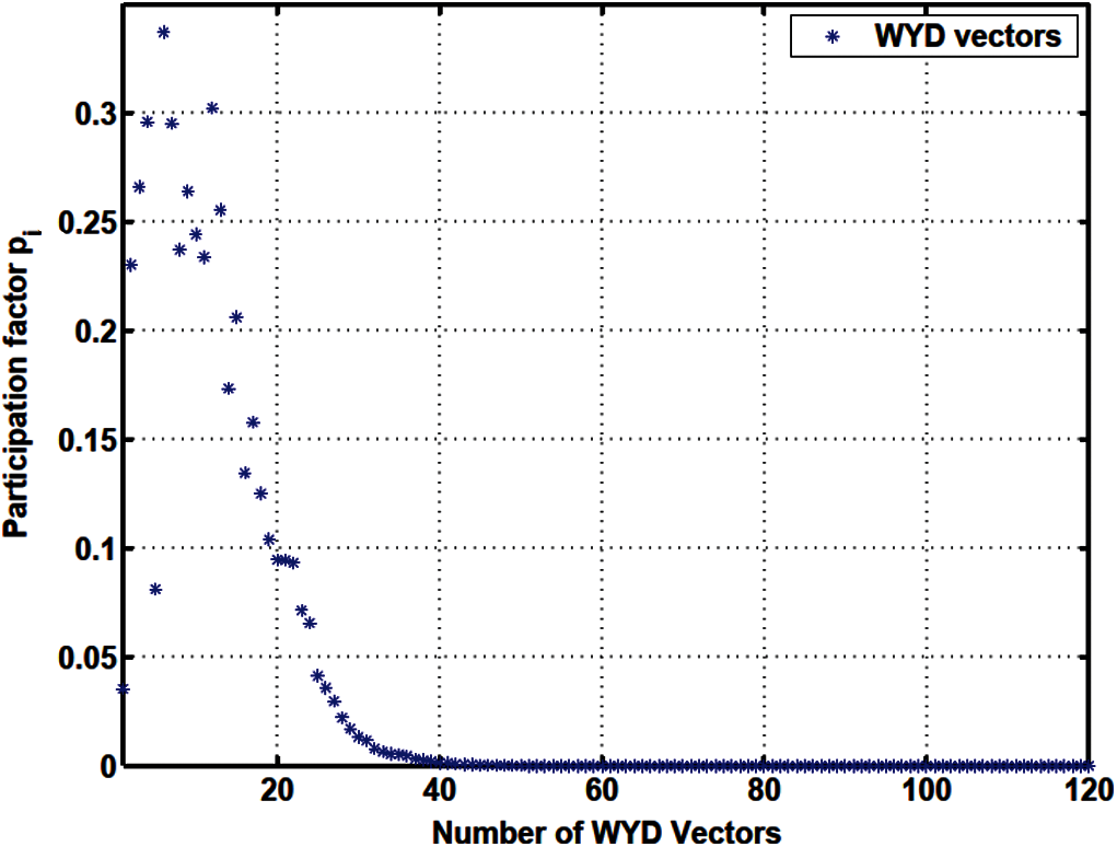
Figure 14: Projected load piW vs. WYD vector number (Sections 2.3.2, 2.4.2): Only the first 120 trial vectors among the 215 trial vectors are shown

The apparent randomness in the projected loads pi and in the load participation factors β i in the Lanczos method (Figs. 11–13) and in the original Falk method (Figs. 17–19), as compared to the smoother projected loads in the WYD method (Figs. 14–16), and in the GFM (Figs. 20–22), is clearly a result of the random starting vectors used in the Lanczos process.

For the WYD method, the projected loads pi and the load participation factors β i start at low values for the static solution, then increase for subsequently generated trial vectors up to some maximum values, then decrease almost monotonically for all subsequent trial vectors. From approximately the 40th trial vector on, the values of pi and of β i in the WYD method are practically zero.

For the GFM, the projected loads pi and the load participation factors β i have significant values concentrated mostly in the first few trial vectors (less than 10).

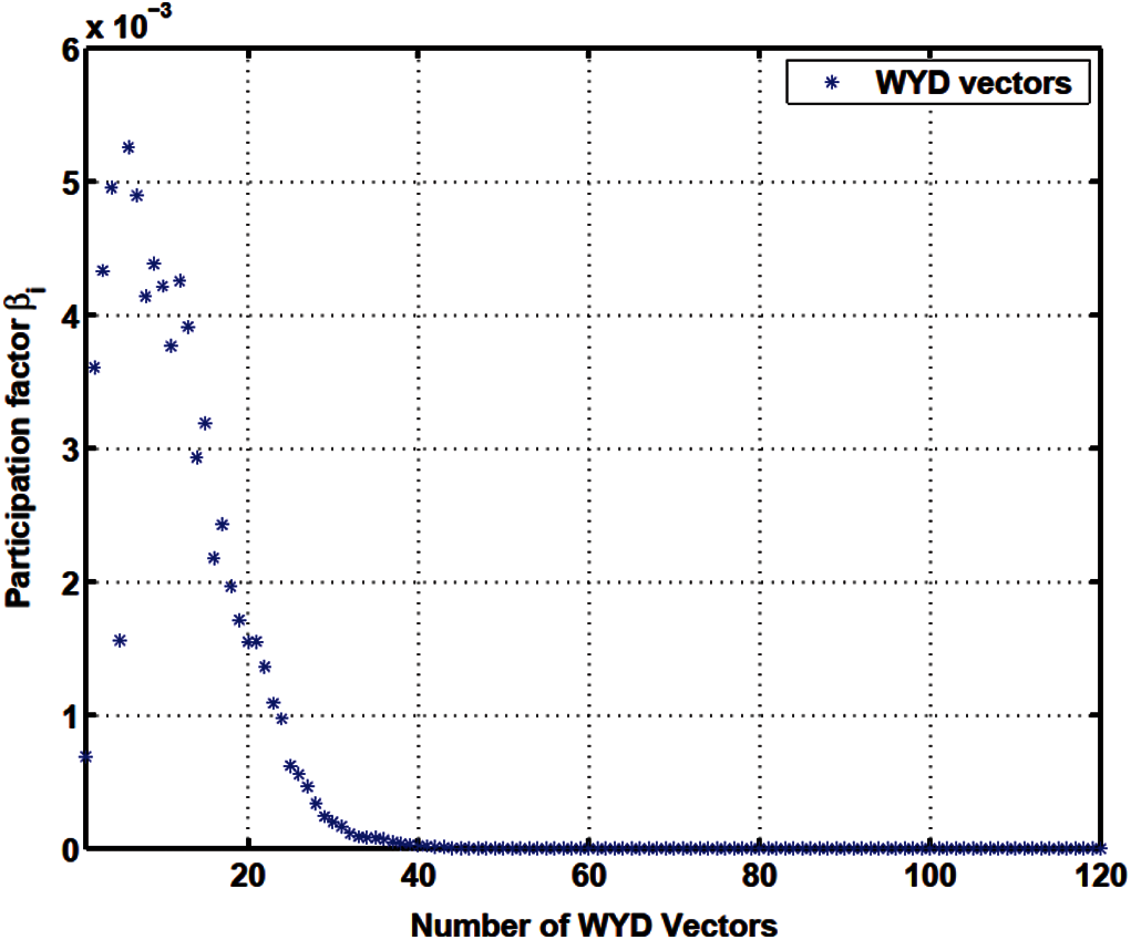
Figure 15: Load participation factor βiW vs. WYD vector number (Section 2.4.2). Only first 120 trial vectors among 215 trial vectors are shown

The response participation factors αi should be used as indicators to select the participating trial vectors for model reduction. For the Lanczos and WYD methods, the response participation factors αi (Fig. 13 for Lanczos, and Fig. 16 for WYD) have significant values concentrated in the first few trial vectors, as opposed to the more spread-out projected loads pi (Fig. 11 for Lanczos, and Fig. 14 for WYD) and load participation factors β i (Fig. 12 for Lanczos, and Fig. 15 for WYD). On the other hand, the response participation factors αi for both the Falk method (Fig. 19) and the GFM (Fig. 22) are spread out over some 50 trial vectors, while the projected loads pi (Fig. 17 for Falk, and Fig. 20 for GFM) and the load participation factors β i (Fig. 18 for Falk, and Fig. 21 for GFM) are more concentrated in the first few trial vectors. It should also be noted that the response participation factor αi in the GFM decrease monotonically and faster as the trial-vector number increases, compared to those in the Falk method in its original form.

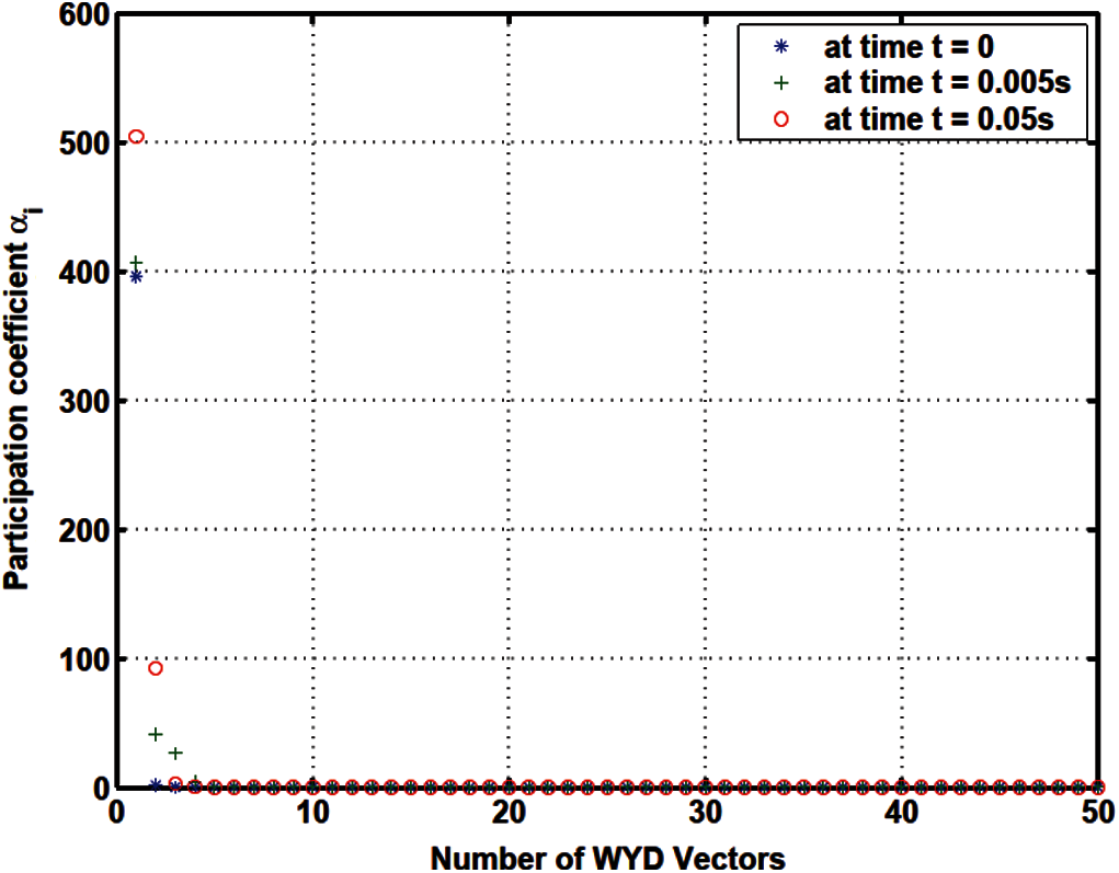
Figure 16: Response participation factor αiW vs. WYD vector number (Section 2.4.2). Only first 50 trial vectors among 215 trial vectors are shown

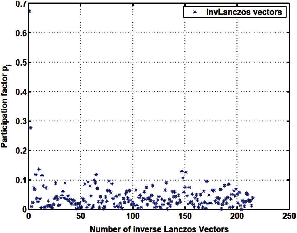
Figure 17: Projected load piF vs. Falk vector number (Section 2.4.2)

Finally, because the transformed matrices have the tridiagonal structure, the reduced-order models in the Lanczos method and in the GFM require less time to solve than that in the WYD method (Fig. 23). The accuracy of these methods are compared in Fig. 24, where the error norm was plotted in terns of the number of trial vectors retained. The WYD method converges fastest, followed by the GFM, then the Lanczos method, and the Falk method. The GFM method converges faster than the Lanczos method, e.g., the error for the GFM with 10 retained trial vectors is equivalent to that of the Lanczos method with 30 to 40 retained trial vectors, as indicated by the red line in Fig. 24. A comparison of Figs. 23 and 24, together with all previous Fig. 11 to Fig. 22, thus reveals a clear niche for the GFM.

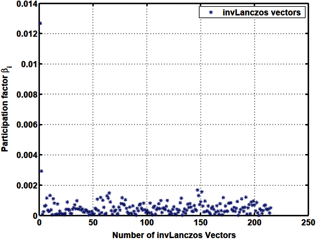
Figure 18: Load participation factor βiF vs. Falk vector number. (Section 2.4.2)

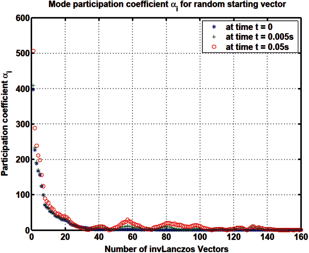
Figure 19: Response participation factor αiF vs. Falk vector number (Section 2.4.2). Only the first 160 trial vectors among the 215 trial vectors are shown

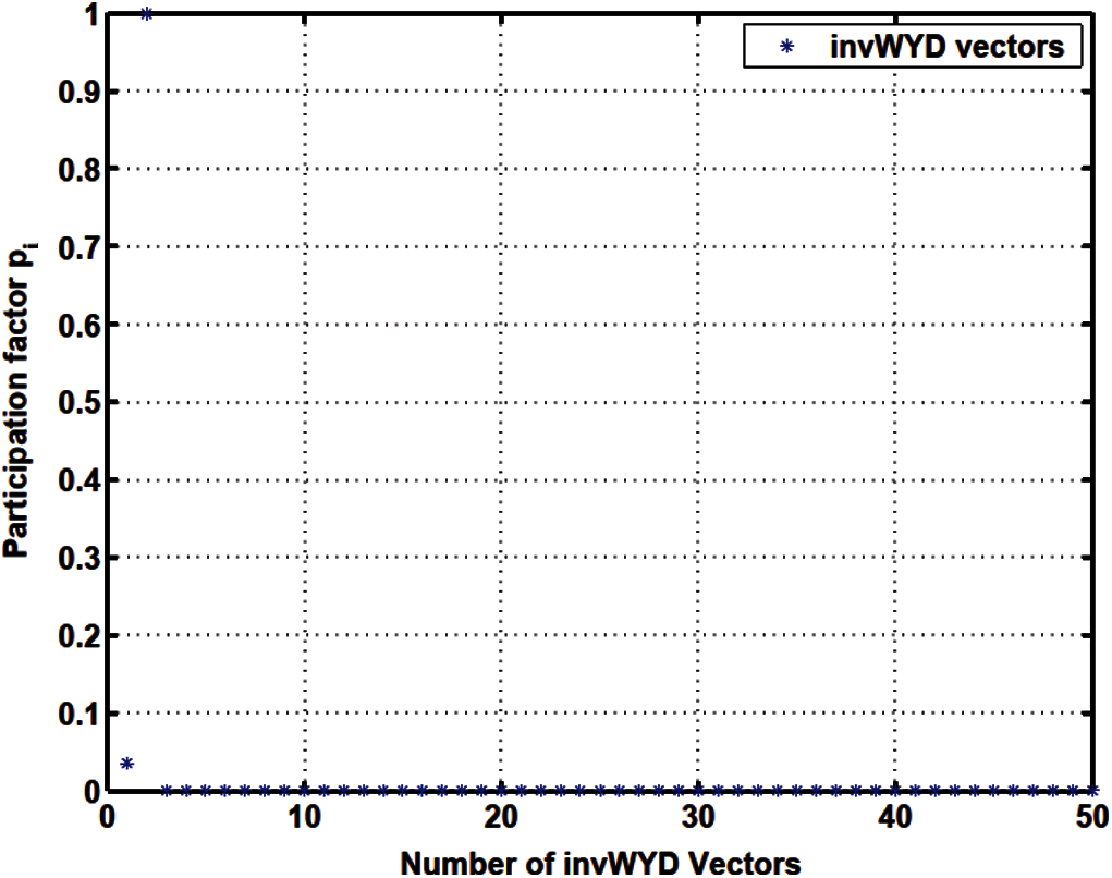
Figure 20: Projected load piG vs. GFM number (Section 2.4.2). Only the first 50 trial vectors among the 215 trial vectors are shown

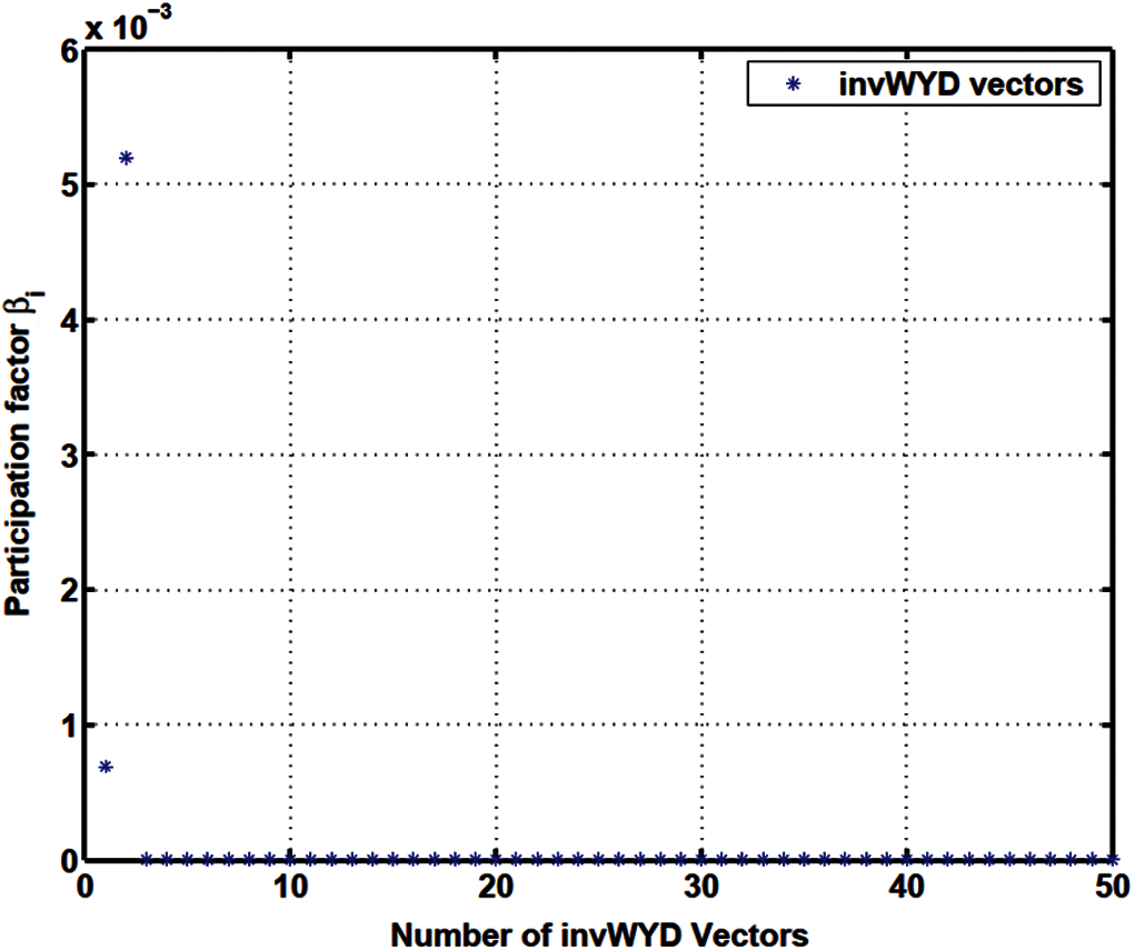
Figure 21: Load participation factor βiG vs. GFM vector number (Section 2.4.2): Only first 50 trial vectors among 215 trial vectors are shown

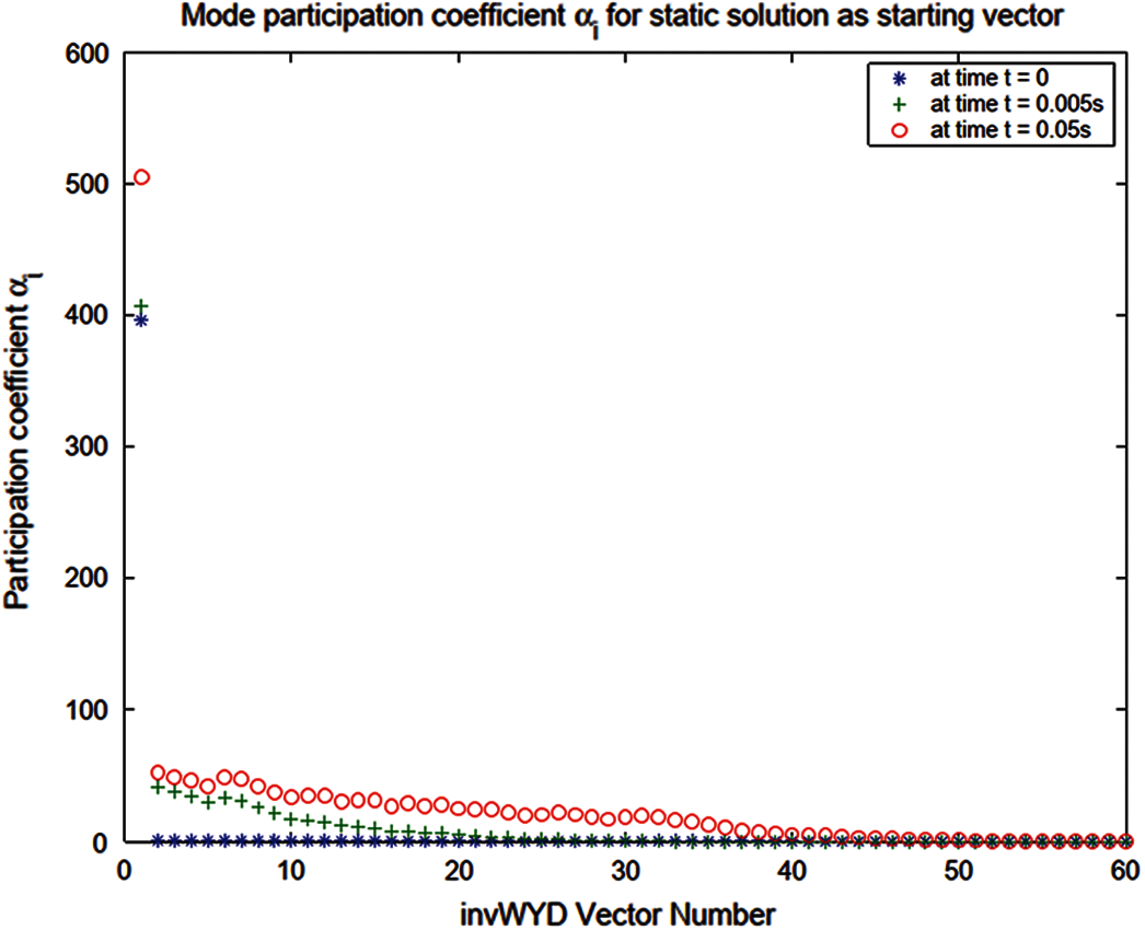
Figure 22: Response participation factor αiG vs. GFM vector number (Section 2.4.2): Only first 60 trial vectors among 215 trial vectors are shown

Also note that for the heat conduction problem the response participation factors αi vary with time, but their magnitude relative to each other remain the same, see Fig. 13 (Lanczos), Fig. 16 (WYD), Fig. 19 (Falk) and Fig. 22 (GFM).

2.5 Two Model-Reduction Strategies

Based on the algorithms presented above, several model-reduction strategies using a combination of the above four methods can be introduced. Two strategies are suggested below.

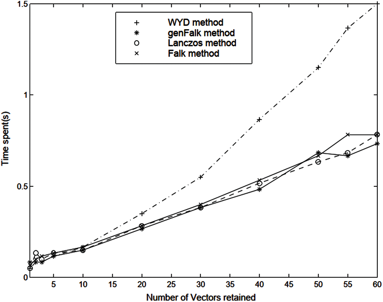
Figure 23: Simulation time for various reduced models vs. trial-vector number (Section 2.4.2)

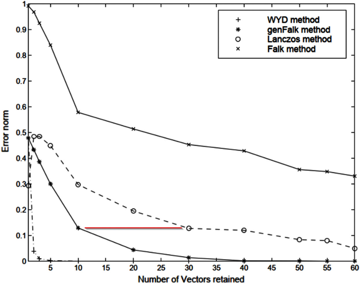
Figure 24: Comparison of error norm vs. trial-vector number (Section 2.4.2)

The first strategy consists of (i) using the WYD method to obtain a reduced-order model by truncating the generation of the WYD trial vectors, followed by (ii) the use of the GFM to transform the resulting reduced-order model to a very simple form (identity capacitance, tridiagonal conductance, Fig. 25), as discussed in the previous sections. Actually, we can even obtain a further reduced-order model by truncating the generation of the GFM trial vectors.

Recall that such truncation can be based on the use of the response participation factor αi discussed above. At the end of this two-stage model-reduction strategy, we obtain a reduced-order model with an identity capacitance matrix and a tridiagonal conductance matrix, which is represented by a simple 1-D equivalent circuit, as discussed in the next sections.

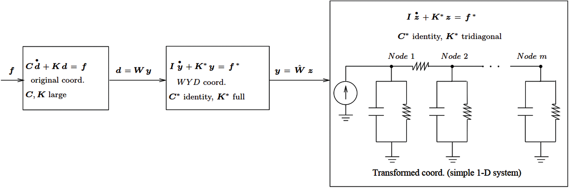
Figure 25: Two-step model reduction strategy (Section 2.5). Strategy 1: The first Step consists of using the WYD method, whereas the second Step relies on the GFM method. Strategy 2: The first Step is based on the Lanczos method, and the second Step on the original Falk method

The second model-reduction strategy is based on the Lanczos and the original Falk methods. The first strategy based on the WYD and GFM methods is more stable than the second strategy based on the Lanczos and Falk methods, especially if the eigenspectrum has close eigenvalues.

Coupled Circuit-Thermal Simulation with Transformed Systems

3.1 Transistor-Thermal Model

In our case-study of electrothermal simulation of circuits with semiconductor devices (e.g., discrete IGBTs or MOSFETs), the circuit network model, the semiconductor device models, and the equivalent thermal circuit network modeling the heat sinks are all coupled together, and solved in a circuit simulator. The electrothermal semiconductor models use the instantaneous device temperature (temperature at the silicon chip surface dnode) to evaluate the temperature-dependent properties of silicon and the temperature-dependent model parameters. These temperature-dependent values are then used by the physics-based semiconductor device models to describe the instantaneous electrical characteristics and the instantaneous dissipated power. In [22 , 54], we proposed a methodology to develop equivalent thermal circuit networks based on a finite-element discretization of the heat-diffusion equation over the domain of the heat sink. Once a thermal network component is developed, and connected to the electrical networks of power electronic systems to provide complete electrothermal models that can be conveniently used in any circuit simulator, it can be used over and over again in many other electrothermal circuit simulation problems.

3.2 Equivalent Circuits for Thermal Part

The methodology developed in [15, 22] could lead to complex thermal networks that present some challenge to implement in circuit simulators such as SABER. If we could transform the original discrete field model into a simple equivalent model, having simple circuit representation that can be easily implemented in any circuit simulator, then we would have considerably simplified the building of the models in coupled field-circuit simulation problems. Indeed, as already mentioned above, the coordinate transformation methods developed in the previous sections can transform any complex thermal model into an extremely simple (1-D) model represented by the “1-D” circuit shown in Fig. 26 (Lanczos) and Fig. 27 (GFM).

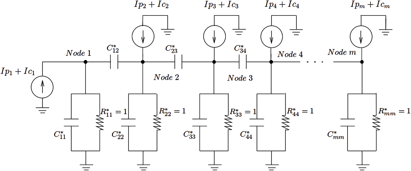
Figure 26: Equivalent circuit by Lanczos method (Section 3.2.1)

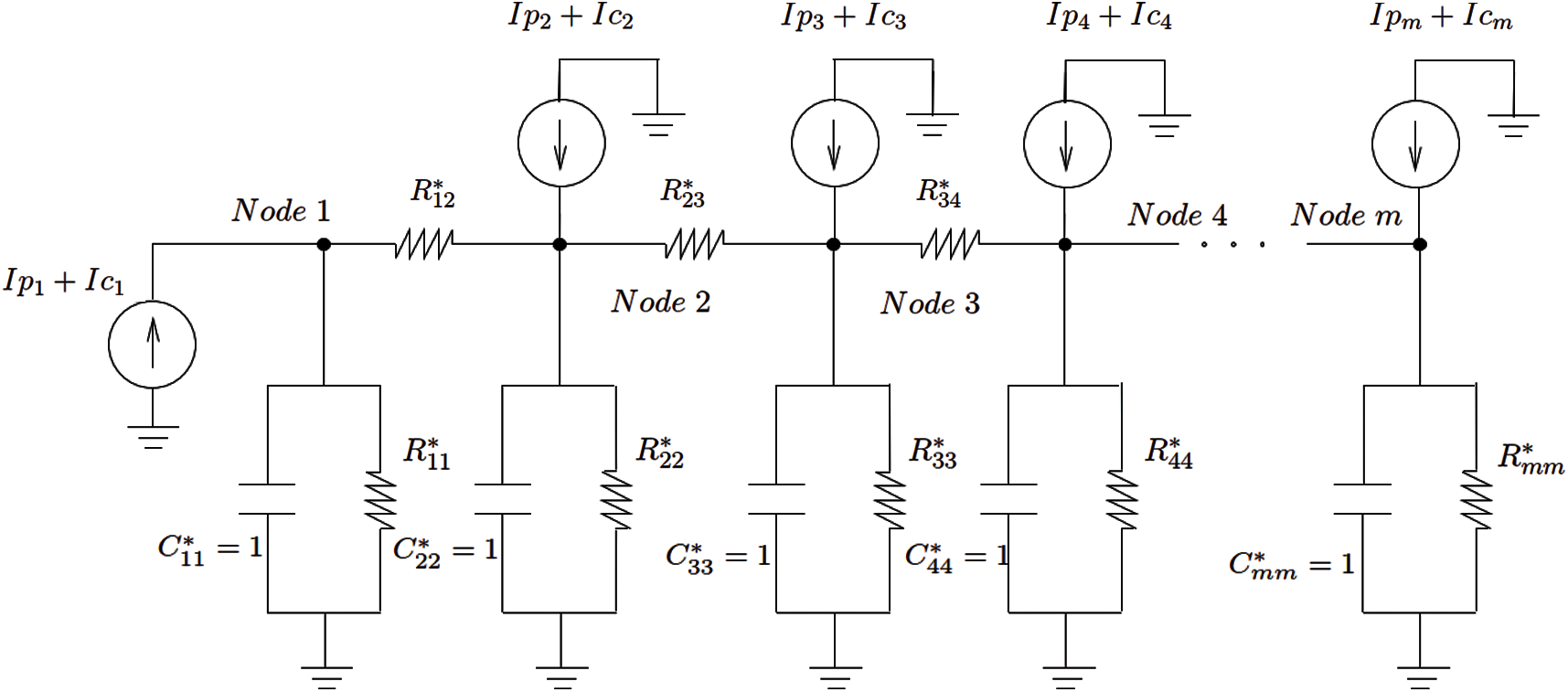
Figure 27: Equivalent circuit by GFM (Section 3.2.2)

Remark 3.1 As presented in [31], the prescribed initial condition Eq. (7) in the new coordinates is computed as follows:

d(0)=Wy(0)⇒y(0)=WTCd(0),(31)

which can be used as input into the circuit simulator SABER, or other any other circuit simulators, as initial nodal voltages. From the physical standpoint, the initial condition can be obtained as the static solution

Kd(0)=f(0)=Ic(32)

where the ambient temperature Ta in the forcing term f(0)=Ic dictates the initial condition. In a circuit simulator, the initial condition as represented by Eq. (32) above is obtained through an initial steady-state solution, prior to the transient solution stage. The modeling of the initial condition in Eq. (5) in our thermal simulation is based on the input initial voltage at each node. From a physical standpoint, before any simulation, SABER solves the steady-state solution first as initial condition. The user then only needs to input the ambient temperature, but does not need to impose the initial voltage at each node. For a general mathematical heat-conduction problem, this is a particular case to bypass the process of reading in an initial condition.

3.2.1 Equivalent Circuit by Lanczos Method

Based on the method for constructing equivalent circuit networks from symmetric matrices in [54], a symmetric global matrix can be decomposed into several elemental matrices, and each elemental matrix represented by a circuit component. A symmetric capacitance matrix C can be realized by a capacitor network, whereas a symmetric conductance matrix K can be realized by a resistor network. After a Lanczos coordinate transformation, the new capacitance matrix Tr becomes tridiagonal, and the conductance matrix K* becomes an identity matrix, Eq. (10) and Appendix A. As a result, in the 1-D equivalent circuit, there is one capacitor in parallel with one resistor between each node and the ground. The capacitance Cii = ci, i −1 +cii + ci, i+1, where ci, i −1, ci, i −1, and ci, i −1 are the coefficients of Tr. The resistor Rii = 1. Between two adjacent nodes i and j, there is a “mutual capacitance” Cij, whose values are the off-diagonal coefficients of Tr, as shown in Fig. 26 (Lanczos), where Ip corresponds to the input power, and Ic the heat-convective boundary conditions, see Eq. (6).

3.2.2 Equivalent Circuit by GFM

Unlike the Lanczos method, the GFM yields an identity capacitance matrix C* and a tridiagonal conductance matrix K*, Eq. (26) and Algorithm 2.1Instead of having the capacitors between two adjacent nodes, we now have the resistors, as shown in Fig. 27. As a result, we have

In addition, there is no capacitor between adjacent nodes since C* is an identity matrix. The resistor between two adjacent nodes is

Again, in Fig. 27, Ip corresponds to the input power, and Ic the heat-convective boundary condition, see Eq. (6).

3.3 Implementation in Circuit Simulators

We have written a MATLAB code to automatically generate element templates13 of the 1-D field networks14 in Fig. 26 (Lanczos transformation) and Fig. 27 (Generalized Falk transformation) for the SABER circuit simulator using the MAST Hardware Description Language15. Models of field packages can be built from these element templates.

A 2-D thermal problem employed in [22] was used to test the simplified circuit networks. Fig. 28 shows the flowchart of our MATLAB code to implement a thermal component model. A finite-element code written in MATLAB for 2-D thermal analysis will generate a 2-D mesh, perform finite element analysis and coordinate transformation by the methods we presented above. The transformed system (transformed capacitance matrix C*, transformed conductance matrix K* and transformed load vector f*) and the trial vectors (W) generated by the coordinate transformation methods will be used to construct the equivalent circuit model (SABER netlist file) and the above mentioned element templates.

Since SABER electrothermal model was constructed to have only one thermal terminal, therefore, we will define only one thermal terminal in our thermal component model by defining the nodal temperature (across variable) and the power input (through variable) at that node as system variables. In general, after coordination transformation, the input power supply in the original idealized physical model as shown in Fig. 10b will distribute out to every node in the transformed model. In other words, the transformed excitation (f*) will have nonzero component in all directions. Therefore, CCCS’s (Current Controlled Current Sources) in the equation section16 of our element templates are used for the power loss from the thermal terminal of the electrothermal model (excitation in the physical coordinate) to control excitations in all other nodes (transformed coordinate).

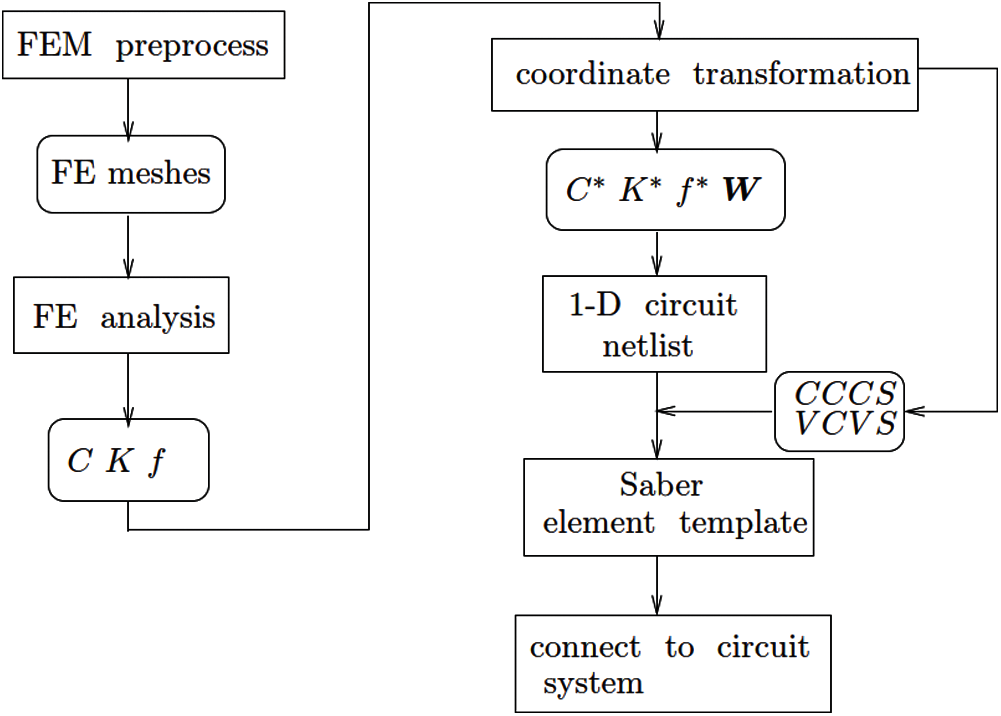
Figure 28: Implementation flowchart. (Section 3.3). MATLAB code flowchart to implement a thermal component model. In the SABER circuit simulator, the Current Controlled Current Sources (CCCS) are used in the element template to connect to the thermal terminal of electrothermal models, and the Voltage Controlled Voltage Sources (VCVC) to obtain the nodal temperatures in the transformed coordinate system, for later recovery back into the physical coordinate system

A typical SABER thermal component template is written as follows:

template heat2d_mesh1 tnode

thermal_c tnode

{

thermal_c y1, y2, y3, y4, y5,…    # local connection point

number p1 = 3.89146e + 01, h1 = 2.30179e-01,

p2 = 4.03557e + 02, h2 = 1.12042e − 01,

…

w1 = 3.89146e + 00,     # trial vector component

w2 = 4.43737e + 01,

…

var i ip     # controlling current

equations

{

p(tnode) += ip

ip: tc(tnode) = w1*tc(y1)+ w2*tc(y2)+…# (VCVS)

p(y1) −= p1*ip + h1     # (CCCS)

p(y2) −= p2*ip + h2     # (CCCS)

…

}

c_th.c1 p:y1 m:0 = 1, 6.96555e + 00

g_th.g1 p:y1 m:0 = 3.75182e − 01

…

netlist which describes the transformed 1-D RC network

}

where : p(tnode) is the across variable at the power input node that will be defined as template thermal terminal, which is physically the temperature at that node. The variable : ip is the through variable at the defined terminal. The variable : ip should also be defined as system variable since all power input at the nodes of the transformed coordinates will be controlled by the CCCS’s via the input power : ip (variable P in Eq. (3), Table 2) at the thermal terminal of the physical coordinates as shown in Fig. 29. From Eq. (18) and Eq. (6), the transformed force can be expressed as

WTf=WTIp+WTIc=p+h.(33)

The above expression is given in matrix form as follows:

WTf=[w1Tw2T…wmT][Ip1Ip2…Ipm]P+[w1Tw2T…wmT][Ic1Ic2…Icm]=[p1p2…pm]P+[h1h2…hm.].(34)

The controlling input power : ip (“P” in Eqs. (3) and (34), Table 2) is used in the CCCSs as follows:

WTf=[p1p2…pm]P+[h1h2…hm]=p+h.(35)

The nodal temperature of the defined thermal terminal will be recovered from the transformed coordinates to the physical coordinates by a VCVS written in the above equation section of the element template. Basically, it is the coordinate-transformation equation at that node:

dnode=∑j=1mwjyj=w1y1+w2y2+…+wmym(36)

where y={y1,y2,…,ym}T is the temperature at the defined thermal terminal in the transformed coordinates.

Table 2 gives the correspondence between the system variables used in our formulation and those used in our MATLAB or SABER implementation.

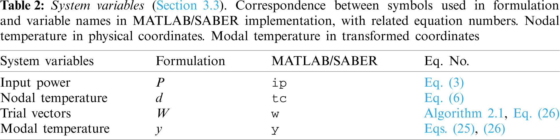
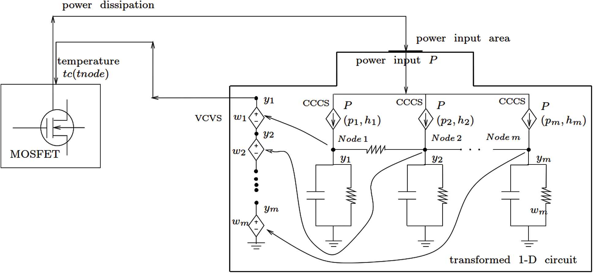
Figure 29: Implementation of the 1-D equivalent circuit in SABER (Section 3.3). See Fig. 10b for the idealized physical domain, Fig. 30 for the overall schematic of equivalent electrothermal circuit network, and Table 2

3.4 Connection to Other Circuit Components

The input power to the thermal system is supplied from the thermal terminal of the electrothermal semiconductor model via the defined thermal terminal of the thermal component model template. The thermal terminal of the semiconductor electrothermal model is thus connected to only the thermal terminal of the thermal component model. By defining the power flowing into the thermal terminal of the thermal component model as system variable, the calculated nodal temperature is dynamically coupled to the semiconductor model.

In Fig. 30, the original complex equivalent thermal circuit network is first transformed by the trial vector basis as d = Wy, Eq. (25), into a 1-D simple equivalent circuit network by our proposed methodology, and the transformation in SABER is implemented by the CCCS’s and VCVS as explained above. The nodal temperature in the transformed coordinates is solved by the SABER built-in efficient numerical solver. The solved nodal temperatures in y in the transformed coordinates is then recovered back to the physical coordinates d using the same trial vectors. Fig. 29 shows the schematic representation of the implementation of the 1-D equivalent circuit into SABER.

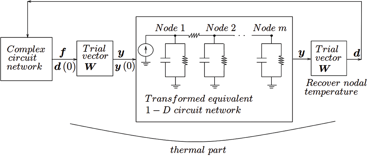
Figure 30: Schematic of equivalent electrothermal circuit network (Section 3.3). The thermal part becomes a simple 1-D circuit network after coordinate transformation. See Fig. 29 for implementation in SABER circuit simulator

Numerical Examples with Model Reduction and Transformation

In this section, we apply the model reduction strategies presented above to extract the reduced-order circuit models for the field component in coupled field-circuit problems to illustrate the efficiency of the proposed methodology. Simulation times for both full-order models and for the reduced-order models are presented for comparison.

4.1 Coupled Transistor-Thermal Models, Verification

The transistor-thermal models obtained from our model-reduction strategies can be verified by considering the 2-D problem in Fig. 10b, showing an Silicon (Si) chip (IGBT or MOSFET) on an idealized TO-247 package. The finite element mesh of this device contains 368 linear triangular elements and 215 nodes.

Used in the analysis are both (1) the full-order model and (2) the reduced-order model obtained by using a combination of WYD method followed by the GFM or the original Falk method. To generate the reduced-order transformed model, a tolerance of TOL = 1E −3 based on the truncation of projected load p defined in Section 2.4, was prescribed in the WYD algorithm, and automatically resulted in a model with 51 nodes, reduced down from 215 nodes. A power of P = 10 W is inputted at the top of the transistor chip, and is distributed uniformly over an area A = 0.1 cm2 (parameter a in Table 4). The circuit simulator SABER and MATLAB were used to implement all developed models, with details of how the full-order model was implemented in SABER described in [54].

Fig. 31 shows a comparison of the transient temperature obtained using the full-order model with m = 215 unknowns, and using a reduced-order model with different numbers r = 11, 31, 41, 51 of retained GFM trial vectors. There is a complete agreement between the two models (full and reduced order) for the temperature at the top of the Si transistor chip.

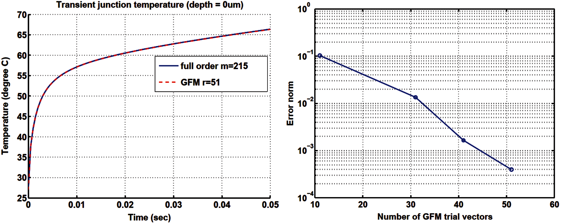
Figure 31: Transient temperature in a pn junction (Section 4.1). GFM reduced-order model vs. full-order model (left). GFM method: Temperature error vs. number of GFM vectors (right)

4.2 Full-Bridge Converter, Electrothermal Simulation

Considerable attention has been focused on switched-mode technology to regulate power supply because it is possible to achieve lossless power conversion to meet the continuing and increasing demand of power electronic devices with reduced size and weight, and with increased efficiency. To turn on and off the flow of energy, and thus achieve regulation, duty-cycle control is employed in switching elements. It has the added advantage when applied to off-line applications of giving significant size reduction in the voltage transformer and energy storage elements, The size of voltage transformer and energy-storage elements in off-line applications can be significantly reduced using switched-mode technology. Such size reduction is another advantage of this technology, in addition to regulating energy flow [48].

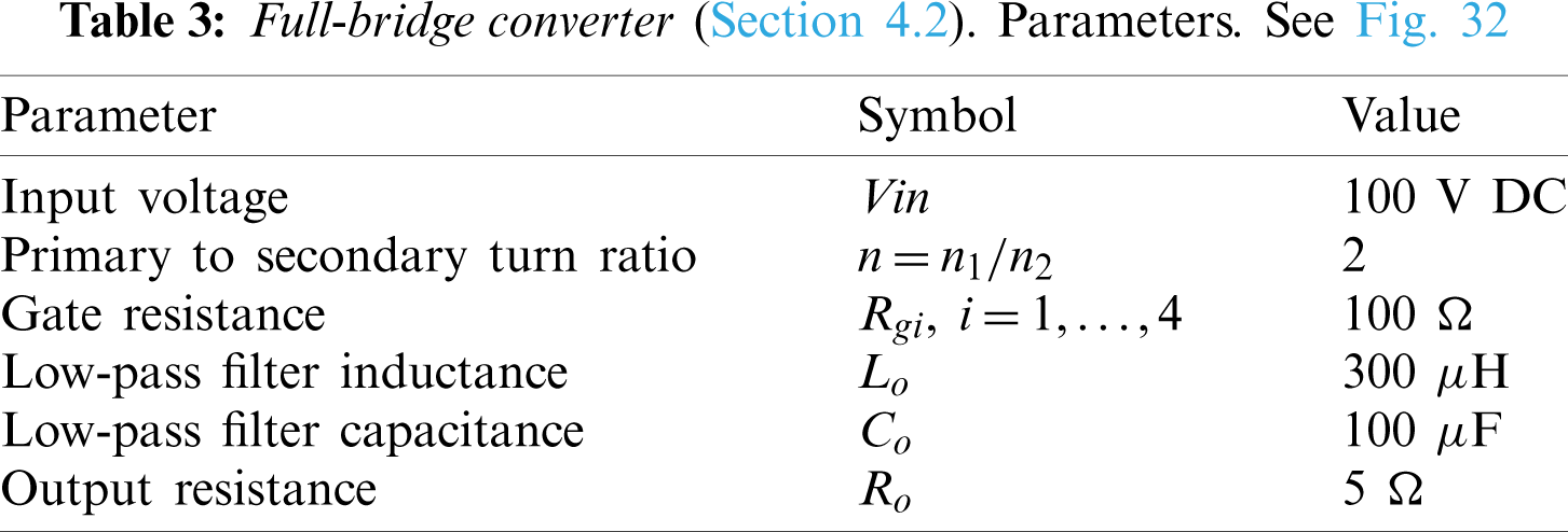
The full-bridge converter is typically used in switching power supplies at power levels of approximately 750 W and greater. A full-bridge buck converter17 with four discrete IGBTs and an isolated transformer, shown in Fig. 32, is simulated with the circuit simulator SABER [22]. The voltages that drive the four discrete IGBTs in the full-bridge buck converter in Fig. 32 are shown in Fig. 33, where the on-time is Ton = 15 μs, the dead-time Δ = 10 μs when all switches are turned off, and the switching-time (or the impulse period) Ts = 50 μs. In the first impulse, lasting for on-time Ton, i.e., the interval 0 < t < Ton, the two discrete IGBT1 and IGBT4 allow current to pass through, while the voltage Vin is inputted into the primary winding of the transformer. The secondary winding of the transformer is center-tapped18, with each half having a voltage of nVin, with n being the ratio of the primary turn over the secondary turn. The positive side of the potential is indicated by a polarity mark (dot). The diode D5 in Fig. 32 is placed to allow the clockwise current flow, from positive pole (indicated by the polarity mark) to negative pole, but prevents the counterclockwise current flow, and is thus called forward-biased. Even though the diode D6 appears to be in the same direction of diode D5, it only allows the counterclockwise current to flow, and is called reverse-biased. Across the filter, the input voltage is therefore nVin, with the filter inductor current i(t) flowing through the diode D5. During the dead-time in the interval Ton < t < Ton + δ, all four discrete IGBTs are switched off, and thus the transformer voltage is Vo = 0 (output voltage). During the time interval Ton + δ < t < Ts − δ, the discrete IGBT2 and IGBT3 and the diode D6 allow current to flow through.

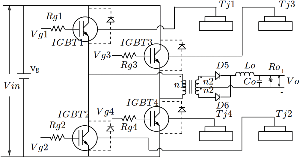
Figure 32: Full-bridge converter (Section 4.2). As a switching device, a full-bridge converter uses four discrecte IGBTs. See Fig. 33 for the time histories of the driving voltages Vg1 to Vg4 for IGBT1 to IGBT4, respectively. See also Tables 3 and 4 for the parameters used

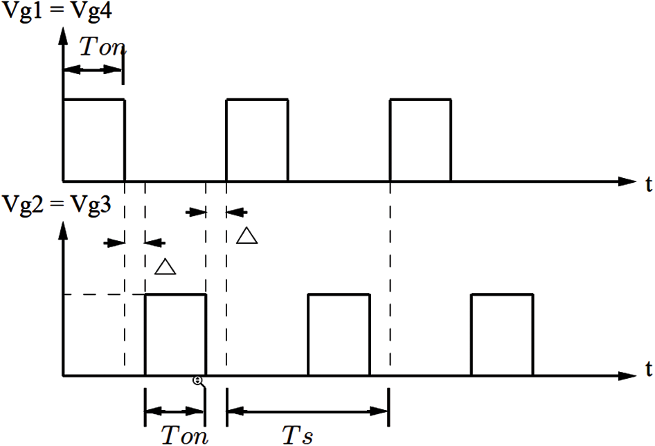
Figure 33: Full-bridge converter (Section 4.2). Waveforms of the driving voltages for the full-bridge converter in Fig. 32 as a switching device. The voltage time history Vg1(t)=Vg4(t) are for the two discrete IGBT1 and IGBT4, and Vg2(t)=Vg3(t) are for IGBT2 and IGBT3

For the full-bridge buck converter in Fig. 32, the parameters were selected as shown in Table 3 so to ensure that a thermal run-away19, which cannot be predicted using a conventional circuit simulator with fixed temperature, would happen.

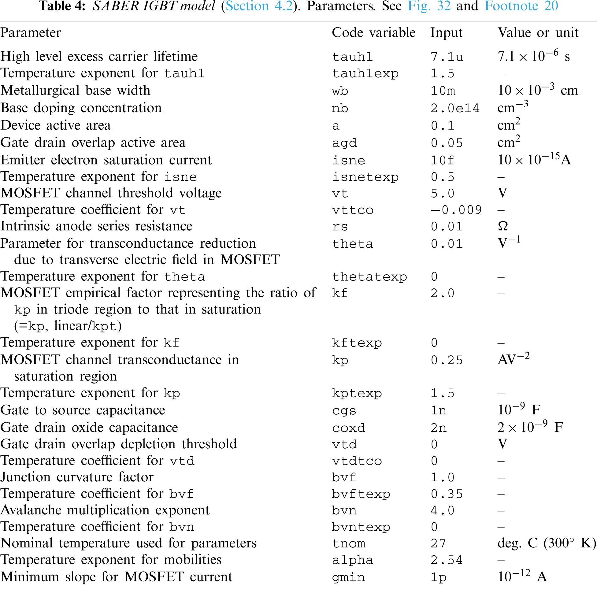
In the circuit simulator SABER, the parameters for the electrothermal IGBT model are shown in Table 4, based on the values suggested in [61 , 62]20. The simulation results of the short-circuit test of the IGBT model using the parameters in Table 4 are similar to those in [63]. The GFM transformed model used here also established the efficiency in coupled transistor-thermal simulations.

Remark 4.1 Since an IGBT is a cross between a bipolar junction transistor (BJT)21 and a MOSFET, there are parameters for MOSFET in Table 4, even though this table is for IGBT parameters, [62]. Before the 1970s, when MOSFET was invented, BJT was the only device used in power electronics. BJT requires high base current to turn on, and slow to turn off, and is subjected to thermal runaway. Unlike BJT, for which the switching is current controlled, MOSFET is voltage controlled, and can limit or stop thermal runaway, and thus became the go-to device in power switch design. IGBT, introduced in the 1980s, has the high-current handling of BJT, and the ease of voltage-control of MOSFET. Generally, IGBT is chosen for low-frequency ( < 20 KHz) and high-voltage ( > 1000 V) applications, whereas MOSFET is chosen for high-frequency ( > 200 KHz) and low-voltage ( < 200 V) applications. In between, either device can be used, depending on application requirements, such as cost, size, speed, thermal specifications22.

The reduced-order model obtained by using a combination of WYD method followed by the GFM23, produced a speed-up factor of close to 9 for the transient-simulation time, compared to the original 2-D-equivalent-circuit thermal full model, as shown in Table 5.

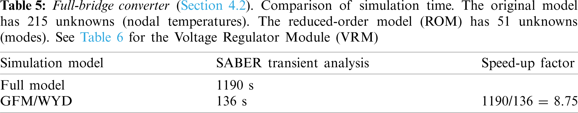
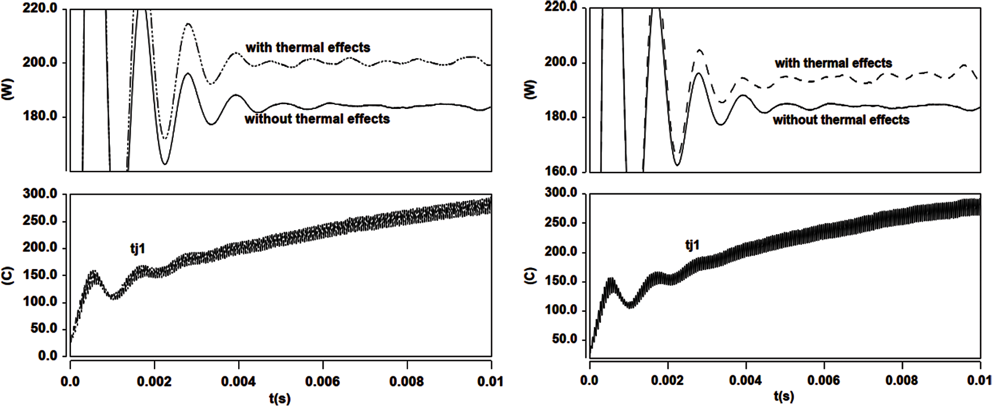
Figure 34: Full bridge converter (Section 4.2). Output power and temperature vs. time. Full-order model (left) vs. GFM reduced-order model (right)

The temperatures Tj1 and Tj2 of the discrete IGBT1 and IGBT2, with heat sink provided by the TO-247 packages, vs. simulation time, together with the time history of the converter output power (Vo * Io), are given in Fig. 34, with and without thermal effects. The result without thermal effects is obtained from the simulation where the Si-chip temperature is fixed to be the ambient temperature. The results clearly show the output power difference between the simulation with thermal effects and that without thermal effects. Such output-power difference would be neglected if we did not incorporate the electro-thermal coupling in the power switching devices into the simulation.

Remark 4.2 In power electronics, the meaning of the term “load” could be confusing. It is best to think of two types of loads: Current load and resistance load. In general, the term “load” is often used to designate “current load”, which is related to output power. Thus “higher load” often means “higher current load”, and thus higher output power. Further, with the relation V = RI, increasing current load corresponds to decreasing resistance load, under constant voltage.

Remark 4.3 A discrete IGBT can be modeled by a resistor, an inductor, and a DC voltage source in series, together with a current switch, controlled by a logical signal, gate on g > 0 or gate off g = 024. In general, for large output voltage, the voltage drop from input to output in IGBT is small. The reason for a small voltage drop across an IGBT device is because this device is roughly equivalent to a voltage source (in series with a resistor and an inductor). Smaller voltage drop in IGBT means larger voltage output which means less power losses. That is why IGBT devices are usually used in higher power applications.

Remark 4.4 Switched-mode semiconductor devices (i.e., IGBT and MOSFET) are employed in high-efficiency power converters. When a semiconductor device operates in the off state, its current is zero and hence its power dissipation is zero. When the semiconductor device operates in the on (saturated) state, its voltage drop is small and hence its power dissipation is also small. In either event, the power dissipated by the semiconductor device is low [48].

4.3 Simulation of a Voltage Regulator Module (VRM)

The ability to work at lower voltage and higher current is required of modern microprocessors to meet the demand of faster and more efficient data processing. Moreover, each modern processor is packed with increasingly more devices, and operates at increasingly higher frequencies. Voltage regulator modules (VRMs) are special on-board power supply modules that minimize the effects of parasitics in interconnections, and can provide highly accurate regulation of supply voltage, as a centralized power system cannot realize these goals. In microprocessors capable of operating at lower voltage and higher current, a VRM located near the load on the motherboard is required [65]. The DC-to-DC converter in a distributed power system produces an intermediate voltage appearing at the computer backplane. Locally regulated low voltages are generated by high-density DC-to-DC converters on each card. Because there is not a lot of space on a crammed motherboard, it is important that on-board converter modules, such as the VRM, be of high power density and high efficiency. A serious design challenge is to have the power conversion perform at high switching frequency to provide fast transient response and to satisfy the requirements of high power density and high efficiency. Each Si chip has an operating output-voltage range, with some tolerance outside of which the chip would fail (blow up). Moreover, there is a voltage range, inside the operating-voltage range, within which the Si chip would be most efficient. For these reasons, the regulated voltage is designed to be fixed.

Fig. 35 shows the circuit schematic of a synchronous rectifier buck-converter used as VRM. The load, represented by the resistor R (i.e., the microprocessor) is powered up from a power supply with regulated output voltage Vg (or Vin). The circuit simulator SABER with our own equivalent circuit model for the idealized TO-247 thermal field component shown in Fig. 10b was employed to simulate the VRM in Fig. 35 [66] with the driving voltage waveforms25 shown in Fig. 36, and with the operating frequency set at 500 kHz. The major VRM components were (Fig. 35 from left to right): Input voltage Vin = Vg = 60 V, MOSFET 1 main switch SW-2XIRF7811, MOSFET 2 synchronous rectifier SR-4XIRF7811, inductor L = 500 nH, output-filter capacitor C = 100 μF, load resistance R = 15 Ω26.

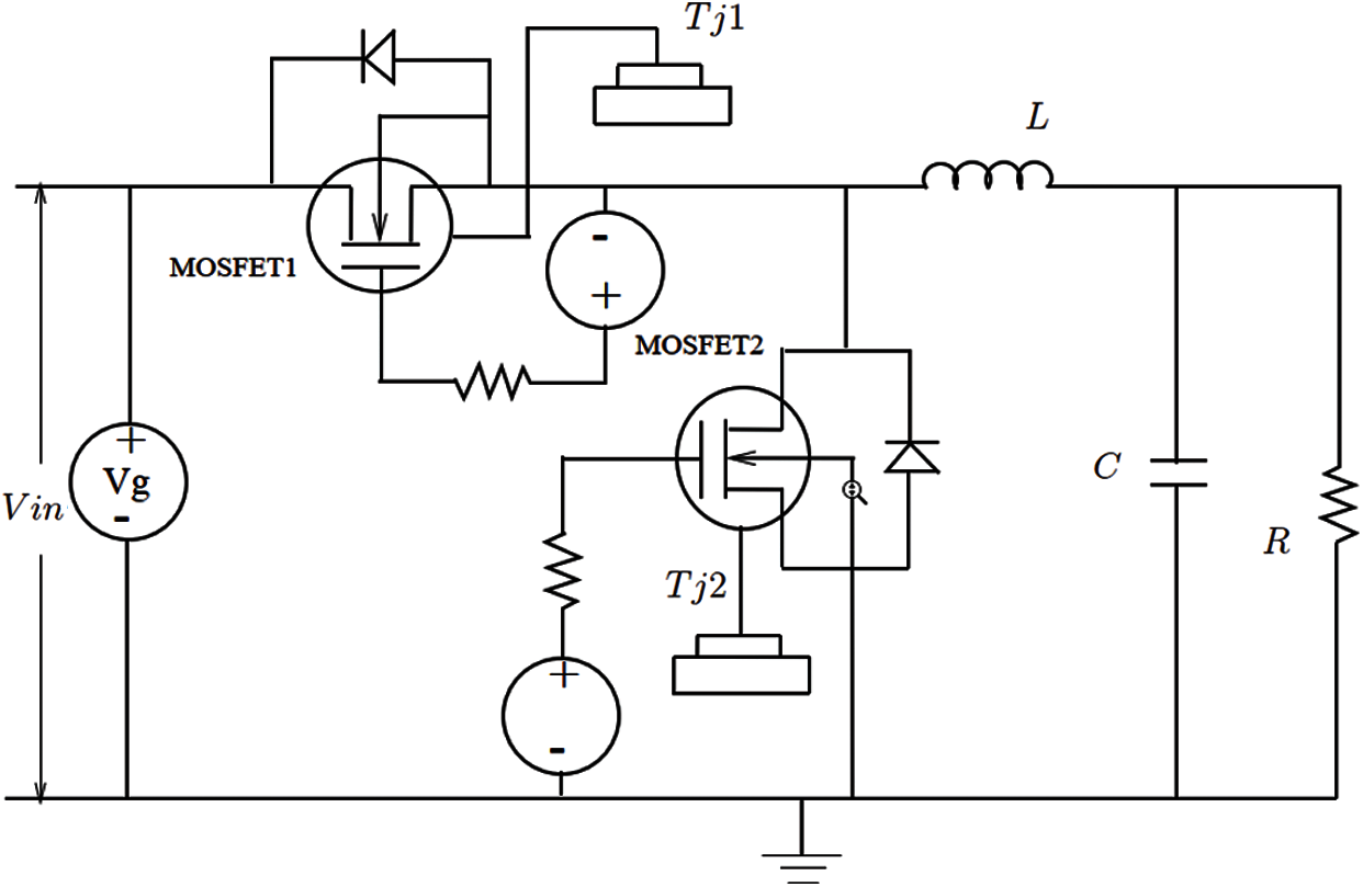
Figure 35: Voltage Regulator Module (VRM) (Section 4.3). Buck converter with synchronous rectifier, with MOSFET1 being the main switch, and MOSFET2 the synchronous rectifier. See Fig. 36 for the time histories of the driving voltages for these MOSFETs. The output voltage Vo is across the resistance R on the right

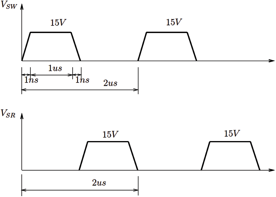
Figure 36: Voltage Regulator Module (VRM) (Section 4.3). Buck converter, driving voltage wave-form excitations VSW (Synchronous Switch, MOSFET1, Fig. 35) and VSR (Synchronous Rectifier, MOSFET2, Fig. 35)

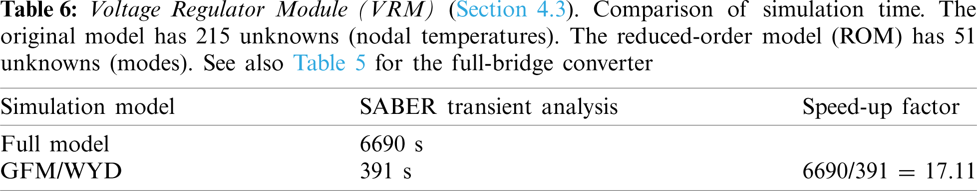
Using the GFM transformed model of the VRM27, the transient simulation time was reduced by 17 times (i.e., the speed-up factor), compared to that of the full two-dimensional thermal model, as documented in Table 6.

Remark 4.5 Most published results in the VLSI-CAD literature to demonstrate simulation speed-up have been in the frequency domain, essentially using methods of the Lanczos type based on the moment-matching technique. Many widely cited papers (e.g., [29, 68]) showed speed-up ratios essentially restricted to the linear part of the circuit (interconnects). On the other hand, the way we computed the speed-up ratio is different: We do not restrict the comparison to the reduced field problem (heat sink) alone, but include the complete field-circuit network in the calculation. If we restricted our calculation of the speed-up ratio to the heat sink alone, we would obtain a much higher speed-up ratio (with orders of magnitude in improvement). The speed-up ratio in our circuit examples, which involved highly nonlinear components (IGBT, MOSFET), was based on the reduction of total simulation time, and not on just the reduction of simulation time for the heat sink (field component), as mentioned above.

4.4 Comparison of CPU Times for Different Methods

In this section, we provide a comparison of the CPU times spent by the full-order models and by two reduced-order models implemented in the circuit simulator SABER.

For a fair comparison between the full-order model and the 1-D transformed models, we need to clock the transformation time in MATLAB. Table 7 shows the MATLAB CPU time spent to generate the transformed 1-D thermal network used in the above simulations. Once the 1-D model had been generated, it can be reused for other design/redesign applications. Such reuse capability is especially advantageous for large complex coupled field-circuit systems.

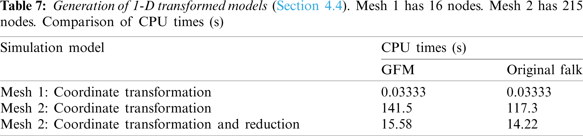
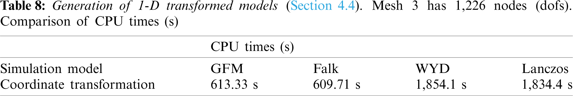
The transformation times for a model of the heat sink (field component) with 1,226 dofs using four different Krylov-based transformation methods considered here, i.e., GFM, original Falk method, WYD method, and Lanczos method, are given in Table 8. The results clearly show that the original Falk method and the GFM are more advantageous than the WYD method and the Lanczos method. The reason is because there is no inversion of the system conductance matrix K in the Falk method and the GFM, in contrast to the WYD method and the Lanczos method.

The results in Fig. 37, obtained from FE Mesh 2 for the buck-converter VRM, show that there was a significant increase in the bulk-drain total energy dissipation of the MOSFET with simulation time, for both the full-order model and the GFM model.

The Si-junction temperature rise and the converter regulated output voltage vs. simulation time are given in Fig. 38. Again, the result without thermal effects is obtained from simulations where the Si-junction temperature is fixed at the ambient temperature. The regulated voltage difference increases with time. Such increase also indicates power dissipation due to thermal effects.

The results show that accounting for the field-circuit coupling is essential for accurate simulations. By applying our proposed model reduction strategies based on the GFM, the speed-up ratio can go up to about 9 for the full bridge converter example (Table 5) and 17 for the VRM example (Table 6), which is highly competitive compared to the traditional Lanczos method.

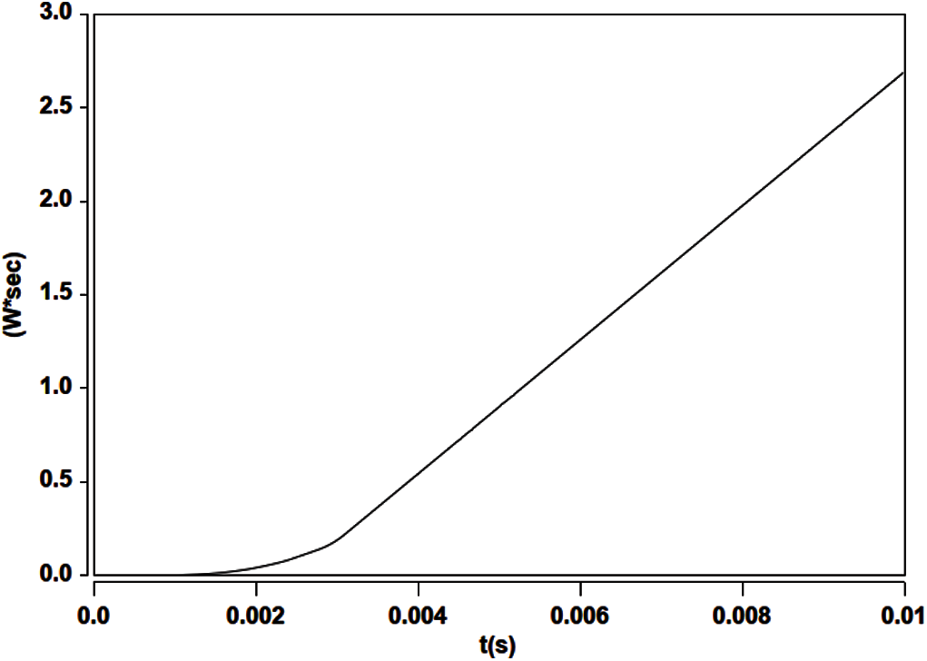
Figure 37: VRM: Total energy dissipation in MOSFET vs. time, using GFM (Mesh 2)

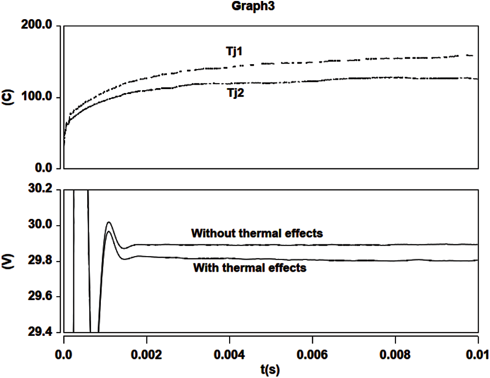
Figure 38: VRM: Si-junction temperature and output voltage vs. time, using GFM (Mesh 2)

Closure

To study truncation effects in the generalized Falk method (GFM) of coordinate transformation, we introduce the concept of response participation factors αi for the selection of trial vectors for model reduction, and show that these response participation factors are more effective than the load participation factors β i traditionally employed. We also compared the simulation times to generate the trial vectors and the error norm committed on the load representation for various coordinate-transformation methods. Unlike the Lanczos method, the GFM does not produce unstable positive poles in circuit simulation, and is more efficient compared to the Lanczos method and the Arnoldi method in the case where a lumped capacitance matrix is used in electrothermal simulation, a case study to illustrate the effectiveness of the proposed methodology for general coupled field-circuit problems, in particular IC interconnects.

At the end of the combined two-stage model-reduction strategy, we obtain a reduced-order model with an identity capacitance matrix and a tridiagonal conductance matrix represented by a simple 1-D equivalent circuit. For the field components in overall coupled field-circuit systems, we develop simple equivalent field circuit networks, which are then implemented in circuit simulators.

Numerical examples of coupled field-circuit problems involving a full-bridge converter with four IGBTs as switching devices and a Voltage Regulator Module with two MOSFETs showed a remarkable efficiency of the proposed coordinate-transformation methods and model-reduction strategies.

1 Proper Generalized Decomposition was used for model-order reduction in nonlinear hydraulic-fracture problems in [15].

2 The Lanczos method is applicable to Hermitian matrices, and is a special case of the Arnoldi method, which is applicable to non-Hermitian matrices.

3 See, e.g., the video “How does an Electric Car work? Tesla Model S” https://Youtube, from time 3:56, where the motor inverter and the induction motor correspond to the motor drive and the electric motor/generator in Fig. 1, respectively. See also “In a Tesla Model S, there is no IGBT packaging trick”, https://Website(Internetarchive), where the brand name on the 3-pin IGBT chip in TO-247 package is International Rectifier (IR), with the circle between the letters I and R being the diagram of a diode drawn vertically; see https://Wikipediaversion09:24,10November2020. International Rectifier was acquired by Infineon (Fig. 5) in 2015. See also p. 17 of the IR 2013 annual presentation to investors https://Onlinepdf (https://Internetarchive) and the video “Pioneers in Clean Technology-Marc Tarpenning-Tesla Motors” https://Youtube at time 1:02:51 when Tarpenning, a Tesla founder, mentioned the new, efficient IGBT by IR, which responded to the need to switch power at 400 V and 1000 Amp for the Tesla.

4 IGBT = Insulated-Gate Bipolar Transistor, “a three-terminal power semiconductor device primarily used as an electronic switch which, as it was developed, came to combine high efficiency and fast switching”; see https://Wikipediaversion11:35,28November2020. See Figs. 5–10 in Section 2.4.

5 A full-bridge converter transform a direct current (DC) at a certain voltage to a DC at a different voltage for use in many electronic devices. See, e.g., the video “Full Bridge Converter-Basics of Switching Power Supplies”, [49], for an explanation of hard switching, soft switching, and phase-shift full-bridge converter.

6 “A voltage regulator module (VRM), sometimes called processor power module (PPM), is a https://buckconverter that provides a microprocessor the appropriate supply voltage, converting +5 V or +12 V to a much lower voltage required by the CPU, allowing processors with different supply voltage to be mounted on the same motherboard. On personal computer (PC) systems, the VRM is typically made up of power MOSFET devices, see https://Wikipediaversion22:07,31December2020. For application of VRM in data centers, see [50].

7 MOSFET = Metal-Oxide-Semiconductor Field-Effect Transistor, is a kind of transistor in which electric field controls current flow, and the device is fabricated by controlled oxidation of silicon semiconductor; see https://Wikipedia23:12,27November2020.

8 Even though the terms “vector” and “column matrix” are used here interchangeably here, the latter is preferred when it adds to clarity.

9 See Fig. 1 in the document ‘TRENCHSTOPTM 5 IGBT (Footnote 4) in a Kelvin Emitter Configuration. Performance Comparison and Design Guidelines’. Application Note Revision 1.0, 2014-10-16, https://Onlinepdf, https://Internetarchive. See also ‘Explanation of discrete IGBTs’ datasheets’. Application Note V1.0, 2015-09-18. https://Onlinepdf, https://Internetarchive. ‘IGBT TRENCHSTOP 5 technology IGZ75N65H5 650 V high speed series 5th generation-Data sheet’, https://Onlinepdf, https://Internetarchive.

10 See ‘Extruded heat sink for PCB mounting’ by Astrel https://Website. https://Internetarchive.

11 A converter transforms AC to DC, whereas an inverter transforms DC to AC.

12 The unit “kVA” or 1,000 Volt-Amperes (VA) is the “apparent power”, proportional to real power measured in “watt” (W) by a “power factor”. “The apparent power equals the product of root mean square voltage and root mean square current. In DC circuits, this product is equal to the real power in watts. Volt-amperes are usually used for analyzing AC circuits. The volt-ampere is dimensionally equivalent to the watt. VA rating is most useful in rating wires and switches (and other power handling equipment) for inductive loads”, https://Wikipediaversion13:20,06January2021.

13 A template is the mathematical description of a subsystem and is contained in a text file. The characteristic equations implemented in a template can be any combination of linear or non-linear algebraic or differential equations.

14 The field networks are the thermal networks in the case study of electrothermal simulations.

15 The MAST Hardware Description Language is the modeling language, originally developed by Analogy, Inc., that allows users to create device simulation models that can be defined in mathematical terms, in any technology, using the native equations and units, without having to resort to electrical equivalents [60].

16 The equation section contains the terminal (connection point) equations of the model, which are often equivalent to the characteristic equations. The relationships involving the through and across variables must be defined in this section [60].

17 The word “buck” came from the fact that the inductor in the circuit always “bucks” or acts against the input voltage. See ‘Buck DC/DC Converters,’ Power Supply Technology, Mouser Electronics https://Website.

18 See the definition of “center-tapped transformer” as a design to allow for two separate voltages with a common connection in https://Multiple-windingtransformers.

19 When an electronic equipment continues to generate heat at a rate faster than the heat can be dissipated, a phenomenon called “thermal run-away”, the equipment would often fail or a fire would break out.

20 See also the default values for the parameters of the n-type IGBT model in the Mathworks Spice circuit simulator. https://Website. https://Internetarchive. SABER numerical inputs use the metric prefix as suffix, e.g., “10f” stands for “10 femto = 10×10−15”; see ‘Metric prefix’, https://Wikipediaversion08:11,19February2021. Among the four references–-[61–64]–-only the conference paper [61] mentioned the coefficients Kp and Kf with the corresponding code variables kp and kf in Table 4.

21 See ‘Bipolar junction transistor’, https://Wikipediaversion15:45,26February2021.

22 See ‘IGBT or MOSFET: Choose wisely,’ by C. Blake and C. Bull, International Rectifier. https://Onlinepdf. https://Internetarchive.

23 The same results were obtained from the original Falk method compared to those from the GFM.

24 See, e.g., ‘IGBT: Implement insulated gate bipolar transistor’, Simscape Electrical version R2020b, Mathworks, https://Website.

25 The results for the VRM are simulations designed to show the difference between model with thermal effects and that without thermal effects. The parameters selected may not be practical. Too small input voltage did not make a significant difference between the cases with and without thermal effects. We changed these parameters to push the electro-thermal model to temperature limits. The input voltage 60 V is for the buck-converter circuit as a whole, not only for the MOSFETs. For more on VRM, see also [67].

26 Shown in Fig. 34 were the junction temperature results using the transformed model. These results were the same for the full model.

27 The same results were obtained using the Falk method in its original form.

Funding Statement: The authors thank the research support of the National Science Foundation.

Conflicts of Interest: The authors declare that they have no conflicts of interest to report regarding the present study.

References

 1.  Lombardi, L., Tao, Y., Nouri, B., Ferranti, F., Antonini, G. et al. (2019). Parameterized model order reduction of delayed PEEC circuits. IEEE Transactions on Electromagnetic Compatibility, 62(3), 859–869. DOI 10.1109/TEMC.2019.2919909.

 2.  Hiruma, S., Igarashi, H. (2020). Model order reduction for linear time-invariant system with symmetric positive-definite matrices: Synthesis of cauer-equivalent circuit. IEEE Transactions on Magnetics, 56(3), 1–8. DOI 10.1109/TMAG.2019.2962665.

 3.  Hasanpour, S., Baghramian, A., Mojallali, H. (2019). Reduced-order small signal modelling of high-order high step-up converters with clamp circuit and voltage multiplier cell. IET Power Electronics, 12(13), 3539–3554. DOI 10.1049/iet-pel.2019.0298.

 4.  Cangellaris, A. C., de Zutter, D. (2004). Special issue on model-order reduction methods for computer-aided design of RF/microwave and mixed-signal integrated circuits and systems-guest editorial. IEEE Transactions on Microwave Theory and Techniques, 52(9), 2197–2198. DOI 10.1109/TMTT.2004.834619.

 5.  Dong, X., Griffo, A., Wang, J. (2020). Multiparameter model order reduction for thermal modeling of power electronics. IEEE Transactions on Power Electronics, 35(8), 8550–8558. DOI 10.1109/TPEL.2020.2965248.

 6.  Acle, Y. G. I., Freitas, F. D., Martins, N., Rommes, J. (2019). Parameter preserving model order reduction of large sparse small-signal electromechanical stability power system models. IEEE Transactions on Power Systems, 34(4), 2814–2824. DOI 10.1109/TPWRS.2019.2898977.

 7.  Wang, Z., Li, Y., Li, Z., Zhao, C., Gao, F. et al. (2019). Reduced-order DC terminal dynamic model for multi-port AC-DC power electronic transformer. Energies, 12(11), 2130. DOI 10.3390/en12112130.

 8.  Nicolini, J. L., Na, D. Y., Teixeira, F. L. (2019). Model order reduction of electromagnetic particle-in-cell kinetic plasma simulations via proper orthogonal decomposition. IEEE Transactions on Plasma Science, 47(12), 5239–5250. DOI 10.1109/TPS.2019.2950377.

 9.  Zimmerling, J., Druskin, V., Zaslavsky, M., Remis, R. F. (2018). Model-order reduction of electromagnetic fields in open domains. Geophysics, 83(2), WB61–WB70. DOI 10.1190/geo2017-0507.1.

10. Zhai, Y., Vu-Quoc, L. (2007). Analysis of power magnetic components with nonlinear static hysteresis: Proper orthogonal decomposition and model reduction. IEEE Transactions on Magnetics, 43(5), 1888–1897. DOI 10.1109/TMAG.2007.892691.

11. Cordesse, P., Remigi, A., Duret, B., Murrone, A., Ménard, T. et al. (2020). Validation strategy of reduced-order two-fluid flow models based on a hierarchy of direct numerical simulations. Flow, Turbulence and Combustion, 105(4), 1381–1411. DOI 10.1007/s10494-020-00154-w.

12. Alfaro-Isac, C., Izquierdo-Estallo, S., Sierra-Pallares, J. (2020). Reduced-order modelling of equations of state using tensor decomposition for robust, accurate and efficient property calculation in high-pressure fluid flow simulations. The Journal of Supercritical Fluids, 165, 104938. DOI 10.1016/j.supflu.2020.104938.

13. Wang, Y., Ma, H., Cai, W., Zhang, H., Cheng, J. et al. (2020). A POD-Galerkin reduced-order model for two-dimensional Rayleigh–Bénard convection with viscoelastic fluid. International Communications in Heat and Mass Transfer, 117(41), 104747. DOI 10.1016/j.icheatmasstransfer.2020.104747.

14. Wang, J., Fang, M., Li, H. (2020). An adaptive substructure-based model order reduction method for nonlinear seismic analysis in opensees. Computer Modeling in Engineering & Sciences, 124(1), 79–106. DOI 10.32604/cmes.2020.09470.

15. Wang, D., Zlotnik, S., Dez, P. (2020). A numerical study on hydraulic fracturing problems via the proper generalized decomposition method. Computer Modeling in Engineering & Sciences, 122(2), 703–720. DOI 10.32604/cmes.2020.08033.

16. Mohan, A., Gaitonde, D. (2018). A deep learning based approach to reduced order modeling for turbulent flow control using LSTM neural networks. https://arxiv.org/abs/1804.09269.

17. Lee, M. W., Dowell, E. H. (2020). Improving the predictable accuracy of fluid Galerkin reduced-order models using two POD bases. Nonlinear Dynamics, 101(2), 1457–1471. DOI 10.1007/s11071-020-05833-x.

18. Sugar-Gabor, O. (2020). Parameterised non-intrusive reduced-order model for general unsteady flow problems using artificial neural networks. International Journal for Numerical Methods in Fluids, 93(5), 1309–1331. DOI 10.1002/fld.4930.

19. Zhong, H., Xiong, Q., Yin, L., Zhang, J., Zhu, Y. et al. (2020). CFD-based reduced-order modeling of fluidized-bed biomass fast pyrolysis using artificial neural network. Renewable Energy, 152, 613–626. DOI 10.1016/j.renene.2020.01.057.

20. Das, A., Khoury, A., Divo, E., Huayamave, V., Ceballos, A. et al. (2020). Real-time thermomechanical modeling of PV cell fabrication via a pod-trained RBF interpolation network. Computer Modeling in Engineering & Sciences, 122(3), 757–777. DOI 10.32604/cmes.2020.08164.

21. Vu-Quoc, L., Humer, A. (2022). Deep learning applied to computational mechanics: A comprehensive review, state of the art, and the classics. Computer Modeling in Engineering & Sciences (to appear).

22. Hsu, J. T., Vu-Quoc, L. (1996). A rational formulation of thermal circuit models for electrothermal simulation-part II: Model reduction techniques. IEEE Transactions on Circuits and Systems Part I: Fundamental Theory and Applications, 43(9), 733–744. DOI 10.1109/81.536743.

23. Lanczos, C. (1950). An iteration method for the solution of the eigenvalue problem of linear differential and integral operators. Journal of Research of the National Bureau of Standards, 45(4), 255–282. DOI 10.6028/jres.045.026.

24. Wilson, E. L., Yuan, M. W., Dickens, J. M. (1982). Dynamic analysis by direct superposition of Ritz vectors. Earthquake Engineering and Structural Dynamics, 10(6), 813–821. DOI 10.1002/(ISSN)1096-9845.

25. Remis, R. F. (2004). Low-frequency model-order reduction of electromagnetic fields without matrix factorization. IEEE Transactions on Microwave Theory and Techniques, 52(9), 2298–2304. DOI 10.1109/TMTT.2004.834577.

26. Wu, H., Cangellaris, A. C. (2004). Model-order reduction of finite-element approximations of passive electromagnetic devices including lumped electrical-circuit models. IEEE Transactions on Microwave Theory and Techniques, 52(9), 2305–2313. DOI 10.1109/TMTT.2004.834582.

27. Xu, J. (1989). An improved method for partial eigensolution of large structures. Computers & Structures, 32(5), 1055–1060. DOI 10.1016/0045-7949(89)90407-0.

28. Bertolini, A. F. (1998). Review of Eigen solution procedures for linear dynamic finite element analysis. Applied Mechanics Review, 51(2), 155–172. DOI 10.1115/1.3098994.

29. Pillage, L. T., Rohrer, R. A. (1990). Asymptotic waveform evaluation for timing analysis. IEEE Transactions on Computer-Aided Design of Integrated Circuits and Systems, 9(4), 352–366. DOI 10.1109/43.45867.

30. Verghese, N. K., Lee, S. S., Allstot, D. J. (1993). A unified approach to simulating thermal and electrical substrate coupling interaction in IC’s. Proceedings of 1993 International Conference on Computer Aided Design, pp. 422–426. IEEE.

31. Vu-Quoc, L., Zhai, Y. H., Ngo, K. D. T. (2004). Efficient simulation of coupled circuit-field problems: Generalized Falk method. IEEE Transactions on Computer-Aided Design of Integrated Circuits and Systems, 23(8), 1209–1219. DOI 10.1109/TCAD.2004.832640.

32. Floros, G., Evmorfopoulos, N., Stamoulis, G. (2020). Frequency-limited reduction of regular and singular circuit models via extended Krylov subspace method. IEEE Transactions on Very Large Scale Integration Systems, 28(7), 1610–1620. DOI 10.1109/TVLSI.2020.2994534.

33. Li, M., Chen, R. (2016). Method of moments wide-band simulations of the microstrip circuits with second-order Arnoldi reduced model. Electronics Letters, 52(10), 841–842. DOI 10.1049/el.2015.2771.

34. Zeng, X. A., Yang, F., Su, Y. F., Cai, W. (2010). NHAR: A non-homogeneous Arnoldi method for fast simulation of RCL circuits with a large number of ports. International Journal of Circuit Theory and Applications, 38(8), 845–865. DOI 10.1002/cta.611.

35. Li, Z., Shi, C. J. R. (2006). A quasi-Newton preconditioned Newton-Krylov method for robust and efficient time-domain integrated circuit simulation. IEEE Transactions on Computer-Aided-Design of Integrated Circuits and Systems, 25(12), 2868–2881. DOI 10.1109/TCAD.2006.882483.

36. Silveira, L., Kamon, M., Elfadel, I., White, J. (1999). A coordinate-transformed Arnoldi algorithm for generating guaranteed stable reduced-order models of RLC circuits. Computer Methods in Applied Mechanics and Engineering, 169(3–4), 377–389. DOI 10.1016/S0045-7825(98)00164-9.

37. Odabasioglu, A., Celik, M., Pileggi, L. T. (1998). PRIMA: Passive reduced-order interconnect macromodeling algorithm. IEEE Transactions on Computer-Aided Design of Integrated Circuits and Systems, 17(8), 645–653. DOI 10.1109/43.712097.

38. Kerns, K. J., Yang, A. T. (1998). Preservation of passivity during RLC network reduction via split congruence transformations. IEEE Transactions on Computer-Aided Design of Integrated Circuits and Systems, 17(7), 582–591. DOI 10.1109/43.709396.

39. Bai, Z., Feldmann, P., Freund, R. (1997). Stable and passive reduced-order models based on partial Padé approximation via the Lanczos process. Technical Report 97/3-10, Bell Laboratories, Lucent Technologies, 700 Mountain Avenue, Murray Hill, NJ 07974-0636.

40. Feldmann, P., Freund, R. W. (1995). Efficient linear circuit analysis by Padé approximation via the Lanczos process. IEEE Transactions on Computer-Aided Design of Integrated Circuits and Systems, 14(5), 639–649. DOI 10.1109/43.384428.

41. Zimmerling, J., Wei, L., Urbach, P., Remis, R. (2016). A Lanczos model-order reduction technique to efficiently simulate electromagnetic wave propagation in dispersive media. Journal of Computational Physics, 315(4), 348–362. DOI 10.1016/j.jcp.2016.03.057.

42. Bracken, J. E., Sun, D., Cendes, Z. (1999). Characterization of electromagnetic devices via reduced-order models. Computer Methods in Applied Mechanics and Engineering, 169(3–4), 311–330. DOI 10.1016/S0045-7825(98)00160-1.

43. Cangellaris, A. C., Zhao, L. (1999). Passive reduced-order modeling of electromagnetic systems. Computer Methods in Applied Mechanics and Engineering, 169(3–4), 345–358. DOI 10.1016/S0045-7825(98)00162-5.

44. Liu, W., Ramm, R. J., Tepe, A. D., Campbell, C. K., Sasaridis, D. (2018). US patent application No. US20180114740A1.

45. Kroeze, R., Campbell, C., Kalayjian, N. R. (2014). Fast switching for power inverter. US patent No. US8760898B2.

46. Un-Noor, F., Padmanaban, S., Mihet-Popa, L., Mollah, M. N., Hossain, E. (2017). A comprehensive study of key electric vehicle (EV) components, technologies, challenges, impacts, and future direction of development. Energies, 10(8), 1217. DOI 10.3390/en10081217.

47. Reimers, J., Dorn-Gomba, L., Mak, C., Emadi, A. (2019). Automotive traction inverters: Current status and future trends. IEEE Transactions on Vehicular Technology, 68(4), 3337–3350. DOI 10.1109/TVT.2019.2897899.

48. Erickson, R. W., Maksimovic, D. (2020). Fundamentals of power electronics. 3rd (ed.). Switzerland AG: Springer Nature.

49. Toshiba Electronic Devices & Storage Corporation, Full Bridge Converter-Basics of Switching Power Supplies-Video Gallery. https://Originalwebsite.

50. Ahmed, M. H., Lee, F. C., Li, Q. (2020). Two-stage 48 V VRM with intermediate bus voltage optimization for data centers. IEEE Journal of Emerging and Selected Topics in Power Electronics, 9(1), 702–715. DOI 10.1109/JESTPE.2020.2976107.

51. Ammous, A., Ghedira, S., Allard, B., Morel, H., Renault, D. (1999). Choosing a thermal model for electrothermal simulation of power semiconductor devices. IEEE Transactions on Power Electronics, 14(2), 300–307. DOI 10.1109/63.750183.

52. Ammous, A., Ammous, K., Morel, H., Allard, B., Bergogne, D. et al. (2000). Electrothermal modeling of IGBT’s: Application to short-circuit conditions. IEEE Transactions on Power Electronics, 15(4), 778–790. DOI 10.1109/63.849049.

53. Hughes, T. J. R. (1987). The finite element method. Englewood Cliffs, NJ: Prentice-Hall.

54. Hsu, J. T., Vu-Quoc, L. (1996). A rational formulation of thermal circuit models for electrothermal simulation-Part I: Finite element method. IEEE Transactions on Circuits and Systems Part I: Fundamental Theory and Applications, 43(9), 721–732. DOI 10.1109/81.536742.

55. Falk, V. S. (1955). Die abbildung eines allgemeinen Schwingungssystems auf eine einfache Schwingerkette. Ingenieur-Archiv, 23(5), 314–328. DOI 10.1007/BF00537495.

56. Paige, C. C. (1972). Computational variants of the Lanczos method for the eigenproblem. Numerical Algorithm, 10(3), 373–381. DOI 10.1093/imamat/10.3.373.

57. Simon, H. D. (1984). The Lanczos algorithm with partial reorthogonalization. Mathematics of Computation, 42(165), 115–142. DOI 10.1090/S0025-5718-1984-0725988-X.

58. Freund, R. W. (1999). Reduced-order modeling techniques based on Krylov subspaces and their use in circuit simulation. Applied and Computational Control, Signals, and Circuits, 1, 435–498. DOI 10.1007/978-1-4612-0571-5.

59. Sridevi, N., Venkatramanan, D., Adapa, A. K., John, V. (2016). Design documentation for four-leg general purpose IGBT converter. Bengaluru, India: Indian Institute of Science, Technical report.

60. Analogy, Inc (1997). SABER users manual. Beaverton, Oregon: Analogy Inc.

61. Hefner, A. R., Diebolt, D. M. (1991). An experimentally verified IGBT model implemented in the Saber circuit simulator. 22nd Annual IEEE Power Electronics Specialists Conference, pp. 10–19. MIT, Cambridge, MA, IEEE. DOI 10.1109/PESC.1991.162645.

62. Hefner, A. R. (1992). Semiconductor measurement technology: INSTANT-IGBT network simulation and transient analysis tool. In: NIST special publication, pp. 400–488. Gaithersburg, MD: National Institute of Standards and Technology.

63. Hefner, A., Blackburn, D. (1993). Simulating the dynamic electrothermal behavior of power electronic circuits and systems. IEEE Transactions on Power Electronics, 8(4), 376–385. DOI 10.1109/63.261007.

64. Hefner, A. R., Diebolt, D. M. (1994). An experimentally verified IGBT model implemented in the saber circuit simulator. IEEE Transactions on Power Electronics, 9(5), 532–542. DOI 10.1109/63.321038.

65. Zhou, X. W., Wong, P. L., Xu, P., Lee, F. C., Huang, A. Q. (2000). Investigation of candidate VRM topologies for future microprocessors. IEEE Transactions on Power Electronics, 15(6), 1172–1182. DOI 10.1109/63.892832.

66. Panov, Y., Jovanovic, M. M. (2000). Design considerations for 12-V/1.5-V, 50-A voltage regulator modules. IEEE Applied Power Electronics Conference and Exposition, vol. 1, 19000210. Piscataway, NJ, USA, New Orleans, LA, USA: IEEE.

67. Shenai, K., Cavallaro, C., Musumeci, S., Pagano, R., Raciti, A. (2003). Modeling low-voltage power MOSFETs as synchronous rectifiers in buck converter applications. 38th Annual Meeting of the Industry-Applications-Society. IEEE, vol. 1–3, pp. 1794–1801. Salt Lake City, UT.

68. Feldmann, P., Freund, R. (1995). Reduced order modeling of large linear subcircuits via a block Lanczos algorithm. Proceedings of the 32nd annual ACM/IEEE Design Automation Conference, Piscataway, NJ, USA, IEEE.

Appendix A. Lanczos method

Lanczos method The Lanczos method [23] was originally proposed as a technique for tridiagonalizing matrices. A sequence of trial vectors are formed by repeatedly multiplying the matrix to be reduced with a starting vector. These trial vectors form a Krylov sequence. Each new trial vector is orthogonalized with respect to the two previous trial vectors. This orthogonalization procedure can be shown to be sufficient to obtain orthogonality with all previously calculated vectors. The coefficients computed from the orthogonalization process are then combined to form a tridiagonal matrix that theoretically has the same eigenvalues as the original matrix, after all n (Lanczos) vectors has been calculated, with n being the order of the system.

Lanczos algorithm

(1) Given C, K∈Rn×n and f∈Rn×1

(2) Triangularize K = LDLT

(3) Starting vector: randomly generated vector z1∗

C-normalize z1∗ to obtain z1

z1=z1∗z1∗TCz1∗∈Rn×1(37)

(4) Solve for additional vectors with b1 = 0 and i = 2,… , r, with r ≤ n:

Kzi∗=Czi−1⇒zi∗=K−1Czi−1∈Rn×1 (38)

ci−1=zi∗TCzi−1 (39)

zi∗∗=zi∗−ci−1zi−1−bi−1zi−2∈Rn×1(C-orthogonalization) (40)

bi=zi∗∗TCzi∗∗ (41)

zi=zi∗∗bi∈Rn×1(C-normalization for zi) (42)

(5) Construct symmetric tridiagonal matrix Tr of reduced order r ≤ n:

Tr=[c1b20…0b2c2b3…00b3c3…00…br−1cr−1br00…brcr]r×r∈Rr×r(43)

(6) Calculate eigenpairs of Tr:

TrY=YΛ∈Rr×r(44)

(7) Approximated eigenpairs of the original system:

X=ZrY∈Rn×r,ωi=1λi,i=1,…,r,(45)

with Zr=[z1,…,zr]∈Rn×r and Y∈Rr×r.

Appendix B. Wilson–Yuan–Dickens (WYD) method

The WYD method, first introduced in [24], has become popular in structural dynamics, and is based on the direct superposition of a special class of Ritz vectors generated from the spatial distribution f(s)∈Rn×1 of the dynamic load that can be put under the form f(s)g(t), where g(t) is function of time. This method eliminates the requirement for exact evaluation of the free vibration frequencies and mode shapes. The WYD approach does not provide a full uncoupling of the equilibrium equations but has proved to be more efficient than the traditional eigensolution approach. The sequence of WYD vectors is generated by taking into account the spatial distribution of the external excitation, which is important information neglected by direct use of exact mode shapes. The first WYD vector is the steady-state vector obtained from a steady-state analysis using the spatial distribution f of the dynamic excitation as input. The other vectors are generated from a recurrence relationship in which the capacitance matrix C is multiplied by the last WYD vector; the resulting vector is then used as the excitation for the next steady-state solution.

WYD Algorithm

(1) Given C, K∈Rn×n, and f∈Rn×1

(2) Triangularize K = LDLT

(3) Solve for load-dependent starting vector w1∗, and C-normalize w1∗ to obtain w1

Kw1∗=f⇒w1∗=K−1f (46)

w1=w1∗w1∗TCw1∗ (47)

(4) Solve for additional vectors i = 2,… , r, with r ≤ n:

Kwi∗=Cwi−1⇒wi∗=K−1Cwi−1 (48)

ci,j=wjTCwi∗ (49)

wi∗∗=wi∗−∑j=1i−1ci,jwj(C-orthogonalization) (50)

bi=wi∗∗TCwi∗∗ (51)

wi=wi∗∗bi(C-normalization to obtain wi) (52)

In the reduced basis of WYD trial vectors, the capacitance matrix Cr∗:=WrTCWr=Ir∈Rr×r is an indentity matrix, whereas the stiffness matrix Kr∗:=WrTKWr∈Rr×r is full in general.

This work is licensed under a Creative Commons Attribution 4.0 International License, which permits unrestricted use, distribution, and reproduction in any medium, provided the original work is properly cited.