Computer Modeling in Engineering & Sciences

DOI: 10.32604/cmes.2021.017944

ARTICLE

The Lu-Pister Multiplicative Decomposition Applied to Thermoelastic Geometrically-Exact Rods

Dedicated to Professor Karl Stark Pister for his 95th birthday

Alexander Humer and Hans Irschik✉

✉Institute of Technical Mechanics, Johannes Kepler University, Altenberger Str. 69, 4040 Linz, Austria
Emails: alexander.humer@jku.at (A. Humer) • ✉hans.irschik@jku.at (H. Irschik)
Received: 18 June 2021; Accepted: 9 August 2021

Introduction

Multiplicative decompositions play an important role in formulating constitutive relations in non-linear mechanics. For a comprehensive review, which discusses multiplicative decompositions in thermoelasticity, plasticity and biomechanics, see Lubarda [1]. In the present paper, which is dedicated to Professor Karl S. Pister on the occasion of his 95th birthday, we particularly refer to a decomposition for thermoelastic solids that was presented by Lu et al. [2]. This multiplicative decomposition of the deformation gradient into a stress-free, intermediate part and a stress-producing, effective part, as well as important consequences drawn in [2] are briefly summarized in Section 2 below. The most important consequence is that the stress tensor associated with a non-isothermal deformation can be determined from the isothermal strain energy simply by replacing the deformation gradient with its effective, stress-producing part. This allows to identify constitutive material parameters in the thermal stress-strain relations by means of isothermal experiments conducted over a range of constant reference temperatures. Following this avenue, we discuss the extension of five isothermal hyperelastic constitutive relations from the literature–-all of them assuming compressibility and isotropy of the material. As in most contributions to compressible thermoelasticity that refer to Lu et al. [2], we utilize energy functions per unit mass in the stress- and deformation-free reference configuration, which we call the Lu-Pister procedure. We exemplary address an alternative formulation based on the concept of the multiplicative decomposition dating back to Stojanovic et al. [3], see Lubarda [1], in which the energy functions are taken per unit mass in the intermediate stress-free configuration. We present a simple relation between the results of the latter formulation and the ones resulting from the Lu-Pister procedure. Subsequently, we focus on the thermal extension of a proven isothermal isotropic, compressible constitutive relation addressed, e.g., in the book on non-linear finite elements by Wriggers [4], and in the book on computational inelasticity by Simo et al. [5]. This isothermal relation belongs to the so-called Simo-Pister class of constitutive relations, see Simo et al. [6] and Hartmann [7]. Utilizing the corresponding thermal relations derived by the Lu-Pister procedure [2], we turn to the geometrically exact Reissner finite-strain beam theory [8]. Our goal here is to bridge a constitutive gap between the structural mechanics type Reissner beam theory and continuum mechanics-type constitutive relations. As opposed to Reissner’s theory [8], in which constitutive relations are to be formulated among stress-resultants (normal and shear force, bending moment) and generalized strains (normal, shear and bending strain), constitutive relations of continuum mechanics are formulated in terms of stresses and strain measures. Unlike structural mechanics, where constitutive relations must be either stipulated or determined by experiments on the actual full-scale structure, standardized small-scale experiments are at disposal on the stress-strain level of continuum mechanics. To exploit the advantages of structural mechanics theories, it is advantageous to derive constitutive relations on the structural level, i.e., among stress-resultants and generalized strains, from stress-strain relations on the continuum level in a preferably consistent way. In the isothermal case, an attempt to bridge this gap has been presented by Irschik et al. [9], see also [10] for beams rigid in shear. In Section 4 below, we first address the Reissner finite-strain beam theory [8] and the isothermal contributions by Irschik et al. [9, 10], which we subsequently extend to thermoelastic problems in Section 5. For this purpose, we derive thermoelastic relations between stress resultants and generalized strains, considering the Simo-Pister-type isothermal stress-strain formulation extended via the Lu-Pister procedure [2]. The efficacy of the proposed approach is illustrated by means of numerical examples of a cantilever subjected to thermo-mechanical loading in Section 6. We compare finite-element solutions of the proposed structural mechanics formulation against results obtained from the corresponding relations of three-dimensional continuum mechanics.

On the Lu-Pister Decomposition for Thermo-Elastic Solids and Its Consequences

Let F denote the thermo-mechanical deformation gradient tensor with the Jacobian determinant

J=detF.(1)

The right Cauchy-Green tensor is

C=FTF.(2)

In [2], Lu et al. [2] introduced the following multiplicative decomposition of F, see their Eq. (14)

F=F¯Fθ,(3)

where Fθ is the deformation gradient belonging to a fictitious stress-free thermal deformation produced by the temperature θ in the current configuration. For thermally isotropic materials, we have

Fθ=Γ(θ)I,(4)

where I denotes the unit tensor, see Eq. (8) of Lu et al. [2]. The Jacobian determinant of Fθ then becomes

Jθ=detFθ=Γ3,(5)

see Eq. (12) of Lu et al. [2]. In Eq. (3), the stress producing part of the deformation gradient is denoted as F. From Eqs. (3) and (4), this so-called effective deformation gradient is obtained as

F¯=Γ−1F(6)

with the effective Jacobian determinant

J¯=Γ−3J.(7)

The effective right Cauchy-Green tensor follows as

C¯=F¯TF¯=Γ−2C,(8)

see Eq. (15) of Lu et al. [2]. In Eq. (9) of [2], Lu and Pister further proposed to express the thermal deformation Γ as

Γ(θ)=exp⁡∫θ0θα(s)ds,(9)

where θ0 is the temperature in the stress-free reference configuration, and α(θ) denotes the coefficient of thermal expansion. In case α is independent of temperature, Eq. (9) gives

Γ(θ)=exp⁡(α(θ−θ0))=exp⁡Θ,(10)

see Eq. (10) of Lu et al. [2]. As was emphasized by Lu et al. [2], the above results are independent of any particular assumptions of material mechanical constitution, except for thermal isotropy. Note that the coefficient of thermal expansion α can be considered as comparatively small for many materials, e.g., it is in the order of 1 × 10−5/K for many metals, and in the order of 1 × 10−4 /K for plastic materials. For sufficiently small values of the dimensionless change in temperature, Θ=α(θ−θ0), i.e., for an infinitesimal thermally actuating strain Θ 1, a linear approximation is sufficient, see Eq. (11) of [2]. Alternatively, an extended approximation, i.e.,

Γn=1+nΘ,(11)

may be used for small absolute values of integers n. On the basis of the multiplicative decomposition for general thermo-mechanical deformations, Eq. (3), Lu et al. [2] concluded that the Helmholtz free energy function ψ for thermo-hyperelastic materials can be expressed as

ψ(C,θ)=W(C¯,θ)+h(θ),(12)

see Eq. (21) of [2]. In the above relation, h is a function of the current temperature θ only; W denotes a strain energy function of isothermal hyperelasticity, in which the effective right Cauchy-Green tensor C¯ substitutes the isothermal counterpart. The argumentation was based on the fact that, since a non-isothermal deformation can be decomposed locally as the product of a free thermal expansion and an effective isothermal deformation, Eq. (3), where the former is taken as stress-free, the stress tensor must depend explicitly on the effective deformation gradient, and thus on C¯ only. As emphasized by Lu et al. [2], the stress tensor associated with non-isothermal deformation can hence be calculated from the isothermal strain energy function W, in which the argument C, however, is replaced by C¯. Indeed, this consequence is not only of highly theoretical but also of practical significance, since isothermal experiments that are conducted over a range of constant reference temperatures are sufficient to identify constitutive material parameters in the stress-strain relations. Setting up a relation to the specific heat, Lu et al. [2] derived the temperature function h(θ) in Eq. (12), see Eqs. (22)–(24) of [2]. This formulation allows a direct determination of h when the specific heat is constant or a function of temperature only. Lu and Pister utilized Cauchy’s stress tensor to formulate constitutive relations, see Eq. (16) of [2]. For our purposes, we will consider the analogous expression for the second Piola-Kirchhoff stress tensor S, which follows by performing the well-known transformation formulas between the two stress measures, see, e.g., Eq. (4.12) of Willner [11], or see Eq. (3.55) of Ziegler [12], and cf. Eq. (5.25) of Parkus [13]. Eventually, we obtain from Eq. (16) of [2] that

S=2ρ0∂ψ∂C=2ρ0∂W¯(C,θ)∂C.(13)

The mass density in the reference configuration is denoted as ρ0. We follow Lu et al.’s [2] notation in the above relation, i.e.,

W(C¯,θ)=W(Γ−2C,θ)=W¯(C,θ),(14)

see their Eq. (19).

Lu et al. [2] particularly exemplified their multiplicative decomposition and its consequences on the case of mechanically incompressible materials. Moreover, they demonstrated that their formulations lead to well-known results under the restrictions of small deformation and temperature change.

Subsequently, we use Eqs. (13) and (14) for a brief discussion on the extension of five isothermal hyperelastic constitutive relations from the literature to the context of thermal stresses, where we will consider compressibility and assume isotropy with respect to the reference configuration. As this is performed in most of the works in the literature on compressible thermo-elasticity, in which reference was made to Lu et al. [2], the free energy ψ and the strain energy function W¯ thereby will be taken as energy functions per unit mass in the stress-and deformation-free reference configuration, such that the reference mass density ρ0 does cancel in the results of Eq. (13). Since this argumentation is also backed by the incompressible and linear examples in [2], we subsequently denote this as the Lu-Pister procedure. We note that alternative formulations were suggested in the literature. We particularly mention the following procedure: As was brought to a wider audience in the review article by Lubarda [1], see also Vujosevic et al. [14], a multiplicative decomposition of the deformation gradient of the type of Eq. (3) was independently suggested earlier by Stojanovic et al. [3]. In this contribution, a constitutive stress-strain relation for the effective elastic deformation with F¯ was introduced with reference to a generally incompatible, stress-free intermediate configuration, which evolves from the reference configuration through Fθ. Counterparts of ψ and W¯ in Eqs. (12) and (13) consequently refer to the intermediate configuration; the fictitious mass density of the latter is taken as ρθ = ρ0Γ−3. This procedure was exemplified for the case of a quadratic dependence of the elastic strain energy on the finite elastic strain, see Eq. (2.18) of Lubarda [1], leading to an isotropic stress-strain law of the St.Venant-Kirchhoff type, i.e., a law that is linear in the effective strain, see Eqs. (2.19) and (2.21) of [1] This law is written for the second Piola-Kirchhoff stress with reference to the stress-free but generally incompatible intermediate configuration with a mass density ρθ. For the total second Piola-Kirchhoff stress tensor S in Eq. (13), which refers to the stress- and deformation-free reference configuration with mass density ρ0, this means that the approach by Stojanovic et al. [3] yields results that are Γ3 times larger than those following from the Lu-Pister procedure [2], in which the energy functions ψ and W¯ in Eq. (13) refer to the reference configuration. We note that this fact holds for any suitable isothermal form of the free energy, not only for the quasi-linear the St. Venant-Kirchhoff model corresponding to Eq. (2.17) of Lubarda [1], which, when substituted into Eq. (2.15) of [1], eventually leads to Eq. (13) above, but with the generally different reference mass density ρθ in the free energy function ψ, see also Eq. (2.18) of [1].

In the following five examples of non-linear constitutive, we restrict ourselves to the Lu-Pister procedure [2]. Only in the fifth case, see Eq. (33) below, in which we discuss the thermal extension of an isothermal constitutive relation frequently addressed in the literature, see, e.g., Eqs. (3.116) and (3.118) of the book on non-linear finite elements by Wriggers [4], and Eq. (7.1.93) of the book on computational inelasticity by Simo et al. [5], we also show the alternative result for the Stojanovic-Djuric-Vujosevic procedure [3]. In conclusion, we think that an alternative use of both procedures allows to compare different non-linear dependencies of the thermal parameter in the thermal extensions of isothermal hyperelastic relations, and thus gives more freedom in constitutive modeling.

On the Perception of the Lu-Pister Decomposition in Literature

A multiplicative decomposition of the deformation gradient as used by Lu et al. [2] in the context of thermoelasticity has also been adopted for the constitutive modeling in other fields of inelastic problems, see the review of Lubarda [1]. We mention applications in finite-strain elastoplasticity, which go back to Lee et al. [15]. Wriggers et al. [16] used multiple multiplicative decompositions combining in their approach to coupled termomechanical problems in elastoplasticity. In the elastic range, assuming isotropy with respect to the reference configuration, it is moreover often assumed that the strain energy W in Eq. (12) can be additively split into a volumetric part Wvol, which is characterized by the bulk modulus K, and an isochoric part Wiso governed by shear modulus μ. Following this concept, which dates back to Flory [17], we may write

W(C¯,θ)=Wvol(C¯,θ)+Wiso(C¯,θ).(15)

Such splitting was used, e.g., for the thermoelastic portion of inelastic non-isothermal deformations by Wriggers et al. [16], who started from a compressible isotropic neo-Hookean formulation originally proposed for large strain isothermal elastoplasticity by Simo et al. [18]. See the doctoral thesis by Miehe [19], and Chapter 6 of the book by Willner [11]. Connecting to the Lu-Pister decomposition, in the latter papers, the volumetric part was taken as

Wvol(C¯,θ)=Wvol,1(C¯,θ)=Kρ012(ln⁡J¯)2,(16)

and the isochoric part was used in the form

Wiso(C¯,θ)=μρ012(trC¯~−3).(17)

Here, C¯~ denotes the isochoric part of the effective right Cauchy-Green tensor C¯,

C¯~=J¯−23C¯=J−23C=C~,(18)

see Eq. (6.184) of Willner [11] and Eq. (6.106) of Miehe [19]. In Eq. (16), we use the index ‘1’ to distinguish the present case from four more constitutive stress-strain models discussed in what follows. The isochoric part in Eq. (17) will remain the same in cases ‘2’ and ‘3’ below, and will not be used in the following cases ‘4’ and ‘5’. Note that in all cases, the strain energy functions are taken in the form of the Lu-Pister procedure, i.e., referring to the mass density ρ0. Only in case ‘5’, we will address and briefly discuss the different result, which follows from the procedure of Stojanovic et al. [3], see Eq. (33) below. Substituting Eqs. (16) and (17) into (14), the result takes on the form

W¯1(C,θ)=Kρ012((ln⁡J)2+2(ln⁡Γ−3)ln⁡J+(ln⁡Γ−3)2)+μρ012(J−23trC−3).(19)

Using the definition of the isochoric part of the effective right Cauchy Green tensor, Eq. (18), we may re-formulate this result as

W¯1(C,θ)=Wvol,1(C,θ)+Wiso(C,θ)+Kρ0(ln⁡Γ−3)ln⁡J+Kρ012(ln⁡Γ−3)2.(20)

The third term on the right-hand side of the above relation represents a thermo-mechanical coupling term, while the fourth one depends on temperature only. With exception of the latter term, the form stated in Eq. (20) coincides with a model used by Armero et al. [20], see their Eqs. (82) and (83). Simo et al. [20] made no use of the multiplicative decomposition by Lu et al. [2]. Instead, an alternative split into an adiabatic elastic phase, in which the entropy of the system is kept constant, followed by a heat conduction phase at fixed configuration, which corresponds to an additive split of the entropy function, was introduced. For related entropy-elasticity considerations applied to isotropic rubber-like solids at finite strains, see Holzapfel et al. [21], who utilized the Lu-Pister decomposition [2] but applied alternative thermodynamic arguments for setting up the thermoelastic free energy, which leads to different formulations, see their Eqs. (25)–(28).

From W¯1(C,θ) in Eq. (20), stresses can be derived utilizing Eqs. (13) and (14). Noting the relations

∂J∂C=12JC−1,∂(trC)∂C=I,(21)

see Table 6.1 of Willner [11], the second Piola-Kirchhoff stresses become

S1=Svol,1+Siso,(22)

where the volumetric part of the thermoelastic stresses follows as

Svol,1=K(ln⁡J+ln⁡Γ−3)C−1,(23)

and the isochoric part becomes

Siso=μJ−23(I−13(trC)C−1),(24)

see also Eq. (6.307) of Willner [11]. The above isothermal counterpart of the strain energy in Eq. (17) was critically studied for the problem of simple tension by Ehlers et al. [22], who showed that it may lead to unphysical response in the case of finite deformations. Indeed, it was shown by Doll et al. [23] that, under isothermal conditions, the above form of the volumetric part Wvol,1 formally fails to satisfy two of nine requirements that should be satisfied, see their Tables 1 and 2. Various other isothermic forms where discussed and extended in the paper by Doll et al. [23], too. We also refer to Kaliske et al. [24] for a discussion of various forms of the isochoric part Wiso. For further discussions and extended formulations concerning the additive splitting of the isothermal strain energy into volumetric and isochoric parts, the reader is referred, e.g., to Hartmann et al. [25], Pence et al. [26] and Moerman et al. [27]. It is to be noted that the various isothermal forms of the strain energy discussed in the above papers [23–27] may be utilized in context with the Lu-Pister decomposition [2] for isotropic thermoelastic deformations in a quite straight-forward manner. Exemplary, we mention the paper by Yosibash et al. [28], where the volumetric part of the strain energy has been formulated according to a suggestion presented by Hartmann et al. [25], which we treat as case ‘2’ now

Wvol,2(C¯,θ)=Kρ0150(J¯5+J¯−5−2)(25)

from which the volumetric part of the second Piola-Kirchhoff stress is obtained as

Svol,2=K110(J¯5+J¯−5)C−1=K110(J5Γ15+Γ15J5)C−1(26)

see Eqs. (8) and (19) of Yosibash et al. [28].

Another formulation frequently adopted for the isothermal volumetric part of the strain energy leads to

Wvol,3(C¯,θ)=Kρ014(J¯2−1−2ln⁡J¯)=Kρ014(Γ−6J2−1−2(ln⁡J+ln⁡Γ−3))(27)

see Eq. (3.122) of the book by Wriggers on nonlinear finite element methods [4] and Eq. (10.4.19) of the book on computational inelasticity by Simo et al. [5]. The corresponding volumetric part of the second Piola-Kirchhoff stress becomes

Svol,3=K12(Γ−6J2−1)C−1(28)

It is to be noted that a complete decoupling into a volumetric and an isochoric part is not required for the multiplicative decomposition and the corresponding consequences introduced by Lu et al. [2]. A class of constitutive relations that does not assume the latter coupling was suggested by Simo et al. [6]. For further discussions, see also Hartmann [7]. As was noted in the latter paper, modeling problems concerning the case of simple shear may be encountered with the Simo-Pister type hyperelasticity relations; nevertheless, they are frequently used in the field of computational mechanics due to their simplicity. In their original paper, Simo et al. [6] explicitly addressed a form of the strain energy, which in the present context of the Lu-Pister decomposition [2] can be written as

W4(C¯,θ)=λρ012(ln⁡J¯)2−μρ0ln⁡J¯+μρ012(trC¯−3),(29)

where λ denotes the second Lamé parameter, see Eqs. (4.2) and (4.4) of Simo et al. [6] and see also Eq. (6.97) by Miehe [19]. Note that the last term in Eq. (29) addresses the total of the effective right Cauchy-Green tensor C¯, and not its isochoric part only. From Eq. (13), the corresponding second Piola-Kirchhoff stress tensor is obtained as

S4=λ(ln⁡J+ln⁡Γ−3)C−1+μ(Γ−2I−C−1).(30)

An alternative isothermal form of the Simo-Pister type, which is related to considerations of Ciarlet [29], and which is frequently addressed in the literature, see Eqs. (3.116) and (3.118) of the book on non-linear finite elements by Wriggers [4], and Eq. (7.1.93) of the book on computational inelasticity by Simo et al. [5], in the present thermal context of the Lu-Pister procedure [2], leads to

W5(C¯,θ)=λρ014(J¯2−1)−1ρ0(λ2+μ)ln⁡J¯+μρ012(trC¯−3).(31)

The above relation gives the second Piola-Kirchhoff stress tensor as

S5=λ2(Γ−6J2−1)C−1+μ(Γ−2I−C−1).(32)

When using the approach introduced by Stojanovic et al. [3], see also Lubarda [1] and Vujosevic et al. [14]–-recall our short discussion given in Section 2 above–-the following alternative result, denoted as S5SDV, is obtained by multiplication with Γ3

S5SDV=λ2(Γ−3J2−Γ3)C−1+μ(ΓI−Γ3C−1)(33)

For comparison sake, we consider two special cases. First, we study the limiting case, in which the deformation is fully constrained, i.e., J→1 and C−1→I. At the same time, we assume that γ becomes very large, i.e., Γ→∞. In this case, S5SDV→(−∞)I, while the components of S5 = −(λ /2+μ)I in Eq. (32) remain finite, albeit at large values. Secondly, assume that the body is free to deform uniaxially and homogeneously, say in x-direction. Let transverse deformations and shear be prohibited. In this case, the axial stretch is Λ = J − 1. For the sake of simplicity, assume that λ = 0, which holds when the Poisson ratio vanishes. The axial component of the second Piola-Kirchhoff stress is taken to vanish, S5, xx = 0, from which we can compute Λ as a function of Γ ≥ 0, for the allowable region Λ > −1. From Eq. (32) we obtain the axial stretch as Λ = −1, while Eq. (33) yields Λ=Γ−1.

We now turn to structural mechanics, in which comparatively thin (slender) structures are approximately described by one- or two-dimensional theories. Thermoelastic cross-sectional stress resultants can be computed in principle by integration over a structure’s cross-section, utilizing, e.g., one of the three-dimensional stress-strain constitutive relations discussed above. In Section 4 below, we give a short discussion of the celebrated finite-strain beam theory by Reissner [8], as well as a short insight into an extension with respect to constitutive modeling of beams starting from the stress-strain level. The latter extension will be used in Section 5 to obtain thermoelastic stress resultants of S5. In Section 5 below, we derive corresponding exemplary results, utilizing the stress response S5 presented in Eq. (32).

On the Reissner’s One-Dimensional Finite-Strain Beam Theory

In [8], Reissner adopted the kinematic assumptions of the classical linear shear-deformable beam theory, i.e., cross-sections remain plane and undistorted in the course of deformation, but not necessarily perpendicular to the deformed axis, see, e.g., Fig. 6.8 of the book by Ziegler [12] on the mechanics of solids and fluids. The corresponding linear theory is usually attributed to Timoshenko, and recently also to Ehrenfest, see the book by Elishakoff [30]. Considering planar deformations, Reissner [8] developed a geometrically non-linear, consistent structural mechanics extension of the Timoshenko beam theory to finite deformations. Reissner’s theory has served as basis of formulations for both planar and spatial problems of beams subjected to large deformation, which are referred to as geometrically exact theories. Exemplarily, we cite the extension of Reissner’s static considerations to dynamics by Simo et al. [31, 32]. An extension to problems of sliding structures based on geometrically exact beam theory was presented by Vu-Quoc et al. [33]. For recent extensions and generalizations of the sliding beam formulation, see Humer et al. [34 , 35].

Subsequently, we consider the plane case as in Reissner’s original paper [8]. Moreover, we restrict ourselves to beams that are initially straight in the reference configuration, which we assume as undeformed, stress-free and with uniform referential temperature θ0. For coordinate systems and notations, see Fig. 1.

Figure 1: Kinematics of shear-deformable beams: The vector r0 describes the position of the beam’s axis in the deformed configuration. It is derivative with respect to the material coordinate r0′ is tangential to the beam’s axis. The rotation of the cross-section is denoted by ϕ and χ is the shear angle. The normal force N and the shear force Q are introduced in the directions of the local frame spanned by the cross-section and its outer normal. The bending moment about the y-axis is denoted by M

Within his geometrically exact beam theory, Reissner [8] showed that constitutive relations on the structural level for the cross-sectional stress resultants must depend on three generalized strain measures, which he denoted as bending strain κ, normal strain ɛ and shear strain γ. In short, Reissner required the bending moment M, normal force N (perpendicular to the cross-section in the current configuration) and shear force Q, see Fig. 1, to be work-conjugate to the generalized coordinates, i.e.,

δWint=Mδκ+Nδε+Qδγ(34)

where δWint is the virtual work of the cross-sectional stress resultants per unit (axial) length in the undeformed configuration. From the principle of virtual work, Reissner concluded that the generalized strainss must obey the following kinematic relations in order to be consistent with the local equilibrium of forces and moments:

κ=φ′,ε=Λcos⁡χ−1,γ=Λsin⁡χ.(35)

In the above relations, Λ is the stretch of the axis and a prime denotes the derivative with respect to the axial coordinate x.

A certain drawback of this formulation is that constitutive relations, see Eq. (4) of [8], must be either stipulated or experimentally determined. As a matter of fact, Reissner made no reference to local constitutive stress-strain relations of continuum mechanics in [8], which means that experiments to identify his constitutive relations need to be made on the actual structure under consideration. As opposed to standardized setups for the identification of stress-strain relations, no small-scale experiments are available on the structural level. Irschik and Gerstmayr attempted to overcome this shortcoming, first for the case of Bernoulli-Euler beams [10], for which the cross-sections are constrained to remain perpendicular to the axis, i.e., χ = 0, and later, in [9], for Reissner’s original relations including shear deformation.

The main idea followed by Irschik et al. [9] to equate Reissner’s virtual work formulation, Eq. (34), with the well-known virtual work density in terms of the scalar tensor product between the second Piola-Kirchhoff stress tensor § and the variation of the Green strain tensor G = (C − I)/2, see Eq. (20) of Irschik et al. [9] and Eq. (3.48) of the book by Washizu [36] on variational formulations in elasticity and plasticity

δWint=∫AS⋅δGdA=12∫AS⋅δCdA.(36)

In the above relation, integration is performed over the cross-section A, which remains plane and undistorted according to Timoshenko’s hypothesis. Irschik et al. [9] showed that the deformation gradient F and the right Cauchy-Green tensor C of Reissner’s theory can be formulated as functions of the generalized coordinates in a comparatively simple form. The Jacobian determinant of the deformation gradient tensor reads

J=1+ε+zκ,(37)

see Eq. (10) of [9]. The component matrix of the right Cauchy-Green tensor in the global Cartesian coordinate system with unit basis vectors ex, ey and ez (Fig. 1) reads

[C]=[J2+γ20γ010γ01](38)

see Eq. (12) of [9]. The components of the inverse C−1 follow as

[C−1]=[1J20−γJ2010−γJ201+γ2J2].(39)

Substituting these kinematic relations into the expression for the virtual work density δWint, Eq. (36), and equating it with Reissner’s counterpart on the structural level, Eq. (34), Irschik et al. [9] in their Eqs. (26)–(28) obtained the following relations for the cross-sectional stress resultants and the components of the second Piola-Kirchhoff stress tensor in the global coordinate system

N=∫ASxxJdA,M=∫ASxxJzdA,Q=∫A(Sxxγ+Szx)dA.(40)

The geometric interpretation of the Cartesian components of the second Piola-Kirchhoff stress tensor as a skew decomposition of the Lagrange stress vectors, see, e.g., Eq. (3.58) in the book by Ziegler [12] and Fig. 5.2 in Parkus’ book on thermoelasticity [13], allowed Irschik et al. [9] to show that the above relations indeed are relations of static equivalence. In their paper [9], Irschik and Gerstmayr utilized the aforementioned isothermal stress-strain relation suggested by Simo et al. [6].

Application of the Lu-Pister Decomposition to Reissner’s Beam Theory

Using the thermo-hyperelastic stress-strain law formulated in Eq. (32), which we have derived as a consequence of the Lu-Pister decomposition [2], we are now in the position to present a stress-strain based thermal extension of the isothermal approach of Irschik et al. [9]. Substituting the kinematic expressions for J and C−1, Eqs. (37) and (39), into the constitutive Eq. (32), the axial component of the second Piola-Kirchhoff stress tensor within the geometrically exact theory follows as

Sxx,5=λ2Γ−6+μΓ−2−(λ2+μ)J−2.(41)

Inserting the above relation in the cross-sectional integral, Eq. (40)1, the normal force N is split into non-thermal and thermal parts

N5=N0,5−Nθ,5,(42)

for which we obtain the relations

N0,5=∫A(λ2+μ)(J−J−1)dA(43)

and

Nθ,5=−∫A(λ2(1−Γ−6)+μ(1−Γ−2))JdA,(44)

respectively. The non-thermal part N0, 5 corresponds to the result presented in Eq. (31) of Irschik et al. [9], and Nθ, 5 represents the actuating influence of the temperature upon the normal force, which vanishes if Θ = 0 and thus γ = 1, see Eq. (10).

Cross-sections of simple geometry admit closed-form solutions of the integrals in Eqs. (43) and (44). We locate the beam’s axis (z = 0) at the centroid of the cross section, such that

∫AzdA=0.(45)

Further, we assume a homogeneous beam and temperature-independent Lamè parameters. For a rectangular beam of height h and are A, we obtain the non-thermal normal force as

N0,5=12(λ+2μ)A(1+ε+1κh(ln⁡(1+ε−κh2)−ln⁡(1+ε+κh2))),(46)

which can be made non-dimensional by relating it to the P-wave modulus P = λ + 2μ and introducing the non-dimensional curvature k = κ h

N0,5PA=12(1+ε+1k(ln⁡(1+ε−k2)−ln⁡(1+ε+k2))).(47)

For a vanishing Poisson ratio, i.e., λ = 0 and the P-wave modulus and Young’s modulus Y coincide, P = 2μ = Y, the non-thermal normal force of a straight beam (k = 0) evaluates to

N0,5YA=12ε(ε+2)ε+1.(48)

If the axial strain ɛ is small, the well-known formula of linear structural mechanics is recovered upon linearization

N0,5YA=ε.(49)

In the classical structural mechanics theory of linear thermo-elastic thin beams, it is often assumed that the cross-sectional temperature dependence can be approximated as being linear in the transverse coordinate z, see, e.g., Chapter IV of the book by Melan et al. [37] and Eq. (6.92) in Ziegler [12]:

Θ=εθ+zkθh,εθ=αTm,kθ=αΔT,(50)

where Tm is the temperature change at the axis relative to the the uniform temperature in the reference configuration, and Δ T denotes the difference of the respective temperature changes at the cross-section’s bottom and top faces. Adopting Eq. (50), which appears reasonable for moderately thick beams, and substituting into the non-linear relation for γ in Eq. (10), in case of temperature-independent material parameters, homogeneous beams and rectangular cross-sections, Eq. (44) takes the closed form

Nθ,5PA=12(1+ε)+λPe−6εθ3(e−3kθ+e3kθ)kθk+(e−3kθ−e3kθ)(6(1+ε)kθ+k)72kθ2+μPe−2εθ(e−kθ+ekθ)kθk+(e−kθ−ekθ)(2(1+ε)kθ+k)4kθ2.(51)

Particularly, for kθ = 0, and assuming the beam remaining straight during deformation, k = 0, we obtain for λ=0→P=2μ=Y that

Nθ,5YA=12(1+ε)(1−e−2εθ).(52)

Alternatively to the strategy of using Eq. (50) in Eq. (44), we may assume that the linear approximation formulated in Eq. (11) for γ and its respective powers, and that the temperature dependence of the material parameters can be again neglected. The latter assumptions allow a connection to the well-known linear formulations of thermo-elastic structural mechanics, which is much more short-handed than the non-linear formulation given in Eq. (51). Setting n = −2 and n = −6, respectively, in Eq. (11), and substituting it into Eq. (44), Nθ, 5 follows for homogeneous beams as

Nθ,5=∫A(3λ+2μ)ΘJdA=(3λ+2μ)∫AΘ(1+ε+zκ)dA,(53)

which leads to significantly simpler relations than (51),

Nθ,5PA=3KP((1+ε)εθ+JyAh2kθk),(54)

where Jy denotes the cross-sectional moment of inertia about the y-axis and K = λ + 2 μ/3 is the bulk modulus. For a rectangular cross-section, the non-dimensional ratio describing the cross-sectional geometry is Ah2/Jy = 12. It is to be emphasized, however, that the approximation of γ according to Eq. (11), while it is appropriate for a wider range of practical situations, may lead to unphysical results for very large deformations. Exemplarily, assume the beam to be statically determinate and to be mechanically unloaded, such that N5 = 0 in Eq. (42). Again, we require the beam to remain straight, i.e., k = 0 and kθ = 0. In this case, ɛ θ can be computed as a function of ɛ. From the sum of the non-thermal and thermal parts of the normal force, Eqs. (48) and (52), respectively, we obtain ɛ θ as

εθ=ln⁡(1+ε).(55)

In the present case, the Jacobian determinant of F becomes J = 1+ɛ. As required, we find a singular behaviour for ε→−1↔J=0, since εθ→−∞ according to Eq. (55). For large normal strains, when ε→∞, Eq. (55) yields εθ→∞, which corresponds to what we expect, i.e., the actuating mean thermal normal strain ɛθ can take any value. If we take the sum of Eqs. (48) and (54) and set N5 = 0 in Eq. (42) instead, we find that

εθ=12ε(ε+2)(ε+1)2.(56)

Again, we obtain εΘ→−∞ in the limiting case of ε→−1, which is what we expect. For large normal strains, however, i.e., ε→∞, the above result yields εθ→1/2. In other words, the actuating thermal normal strain can not be increased beyond that value, which, of course, lacks physical support. For straight beams (k = 0) with rectangular cross-sections and a vanishing Poisson ratio, which implies λ = 0, the above results Eq. (52) boils down to

Nθ,5YA=(1+ε)εθ,(57)

from which we find the classical relations of linear structural mechanics upon neglecting the coupling, i.e.,

Nθ,5YA=εθ,(58)

see Eqs. (XVIII.11) of Parkus [38] and (6.32) of Ziegler [12]. For N5 = 0, The classical linear approximations, Eqs. (49) and give the result ɛ θ = ɛ, which implies that a finite value of ɛ θ = −1 yields ε→−1. We recover the well-known classical deficiency of linear elasto-statics that a finite value of a compressive normal force resulting in J = 0, i.e., the length of the axis element shrinks to zero.

In analogy to the above results for the normal force, we proceed with the constitute equations for the bending moment M. For this purpose, we first split the bending moment into non-thermal and thermal parts

M5=M0,5−Mθ,5.(59)

From the stress response Eq. (41) and the definition of the bending moment (40), we obtain the non-thermal part as

M0,5=∫A(λ2+μ)(J−J−1)zdA,(60)

see Eq. (33) of Irschik et al. [9]. The thermally ‘actuating’ part of the bending moment follows as

Mθ,5=−∫A(λ2(1−Γ−6)+μ(1−Γ−2))JzdA.(61)

Integration over the beam’s cross-section gives a closed-form expression for the (non-dimensional) non-thermal part of the bending moment

M0,5hPJy=−Ah22Jy1k+k2−Ah22Jy1k2(1+ε)(ln⁡(1+ε−k2)−ln⁡(1+ε+k2)).(62)

To connect to classical beam theory, we consider the relation that corresponds to the particular case of pure bending and a vanishing Poisson ratio, which we obtain by setting ɛ θ = ɛ = 0 and λ=0↔P=Y

M0,5hYJy=−Ah22Jy1k+k2−Ah22Jy1k2ln⁡(2−k2+k).(63)

Upon linearization, we recover the well-known non-thermal constitutive equation for the bending moment as

M0,5hYJy=k.(64)

To determine the thermal part of the bending moment, we adopt the same linear approximation for the temperature field, Eq. (50), as for the normal force. For this assumption, the cross-sectional integral Eq. (61) evaluates to the closed-form relation

Mθ,5hPJy=k2+λPe−6εθ6(e−3kθ+e3kθ)kθ(k+3(1+ε)kθ)+(e−3kθ−e3kθ)(6(1+ε)kθ+k(2+9kθ2))36kθ3+μPe−2εθ6(e−kθ+ekθ)kθ(k+(1+ε)kθ)+3(e−kθ−ekθ)(2(1+ε)kθ+k(2+kθ2))2kθ3.(65)

As a particular case, we again study the case of pure bending (ɛ θ = ɛ = 0) and zero Poisson ratio, for which the above relation for the bending moment simplifies to

Mθ,5hYJy=k2+32(e−kθ−ekθ)kkθ3.(66)

Due to the exponential structure of the thermal deformation, see Eq. (10), which was proposed by Lu et al. [2], kθ appears in the exponent of the (non-dimensional) thermal part of the bending moment. Using the linear approximation of the thermal deformation according to Eq. (11), the cross-sectional integral again takes a much simpler structure

Mθ,5=∫A(3λ+2μ)ΘJzdA=(3λ+2μ)∫AΘ(1+ε+zκ)zdA,(67)

from which the thermal part of the bending moment follows as

Mθ,5hPJy=3KP((1+ε)kθ+εθk).(68)

By setting the Poisson ratio zero, i.e., 3K = P = Y, we recover the classical result for the thermal part of the bending moment in beams upon linearization

Mθ,5hYJy=kθ.(69)

As a last point, we address the constitutive relations of shear force Q within our approach, which, again, is split into a non-thermal part and a thermal contribution, i.e.,

Q5=Q0,5−Qθ,5.(70)

For this purpose, we first determine the shear component Szx of the second Piola-Kirchhoff stress tensor within the kinematic assumptions of Reissner’s beam theory

Szx,5=−γλ2Γ−6+γ(λ2+μ)J−2.(71)

Substituting the shear stress along with the normal stress, Eq. (41), into the cross-sectional integral for the shear force, Eq. (40)3, we obtain the non-thermal part as

Q0,5=∫AμγdA=μAγ,Q0,5μA=γ.(72)

In spite of the comparatively complex constitutive model on the continuum level, Eq. (32), the shear force turns out linear in the (generalized) shear strain γ within our approach. For the thermal contribution, we obtain the cross-sectional integral

Qθ,5=∫Aμγ(1−Γ−2)dA.(73)

For a linear temperature distribution over the thickness, see Eq. (50), the integral evaluates to

Qθ,5μA=γ+12γkθe−2εθ(e−kθ−ekθ).(74)

Resorting to the linear approximation of the thermal deformation, Eq. (11), gives the comparatively simple relation

Qθ,5=2∫AμΘγdA,(75)

from which the non-dimensional thermal part of the shear force follows as

Qθ,5μA=2γεθ.(76)

It is to be noted here that no thermal contribution to the shear force appears in the classical linear structural mechanics theories for isotropic homogeneous beams. Our results, Eqs. (74) and (76), however, do lead to a thermal part of the shear force as soon as shear deformation occurs, i.e., γ ≠ 0.

Numerical Example

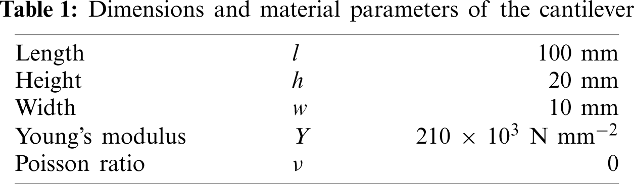
To illustrate the efficacy of our approach, we compare the proposed continuum mechanics-based extension of Reissner’s beam theory against solutions obtained from corresponding three-dimensional relations of thermo-hyperelasticity. For this purpose, we study the fundamental problem of a cantilever under pure thermal loading and combined thermo-mechanical loading, respectively. Fig. 2 (left) shows the undeformed reference configuration of the structure, which is clamped at x = 0. Geometric and material parameters are listed in Table 1.

In particular, we consider the the load cases of uniform thermal bending and combined non-uniform thermo-mechanical loading.

Figure 2: Cantilever subjected to thermal loads: Undeformed reference configuration (left) and deformed configuration (right) under thermal loading by kθ/π = 0.2, which corresponds to a rolling up the straight beam into a semicircle. The right figure shows the actual structured finite-element mesh used in three-dimensional computations, where symmetry with respect to the xz-plane is accounted for

We use finite elements to construct approximate solutions for both the one-dimensional structural mechanics formulation and the three-dimensional relation of continuum thermomechanics. For the structural mechanics relations, which rely on the finite-element formulation for the geometrically exact beam theory by Simo et al. [31, 32], who extended Reissner’s theory to dynamics. The equally simple as efficient formulation of Simo et al. [31, 32] interpolates displacements of the beam’s axis ux, uz and the cross-section’s rotation ϕ, see Fig. 1, using corresponding nodal degrees of freedom. The principle of virtual work (34) serves as basis for the finite-element approximation. Within our extension to thermomechanics, which relies on the Lu-Pister decomposition, Eq. (3) and a continuum mechanics-based derivation of the constitutive equations on the structural level, we use the relations for the normal force N, Eqs. (42), (47) and (51), the bending moment M, Eqs. (59), (62) and (65), and the shear force Q, Eqs. (70), (72) and (74). In the subsequent study, we use two-noded elements with linear shape-functions and reduced integration. A uniform discretization of the cantilever into nx = 40 elements has proven sufficient. A more detailed convergence analysis, however, is beyond the scope of the present paper. Within the structural approach, the clamping is realized by imposing homogeneous boundary conditions on both the displacement field and the cross-section’s rotation at the clamped end

ux(x=0)=0,uz(x=0)=0,φ(x=0)=0.(77)

The finite-element formulation for the three-dimensional problem is based on the continuum mechanics counterpart of the virtual work of the internal forces, Eq. (36), where the Simo-Pister-type stress-response, Eq. (32), is substituted. We use displacement-based finite-elements, in which the three-dimensional displacement field is interpolated by means of hierarchical polynomial shape functions, see, e.g., Zienkiewicz et al. [39]. A structured mesh of nx × ny × nz = 40 × 2 × 8 elements with cubic shape functions is employed in the analysis. At the clamped end x = 0, all components of the displacement field are prohibited, i.e.,

ux(x=0,y,z)=0,uy(x=0,y,z)=0,uz(x=0,y,z)=0.(78)

Both the structural finite-elements and the three-dimensional continuum mechanics formulation are implemented in the general-purpose finite-element code Netgen/NGSolve (https://ngsolve.org).

Thermal Bending of a Cantilever

Within this study, we impose a non-dimensional thermal curvature up to kθ = 0.2π, which corresponds to a linear distribution of the temperature over the beam’s thickness, see Eq. (50), where the change of the mean temperature vanishes, i.e., Tm = 0. Fig. 3 shows the (non-dimensional) components of the tip-displacement ux(x = l), uz(x = l) as a function of the load kθ , where solutions obtained with the proposed thermo-mechanical extension of Reissner’s structural mechanics (SM) formulation are compared against results of the three-dimensional relations of continuum mechanics (CM). The deformed configuration of the cantilever in the final position is illustrated in Fig. 2 (right). Despite the large deformation, results for the tip-displacement obtained with the two distinct approaches agree remarkably well.

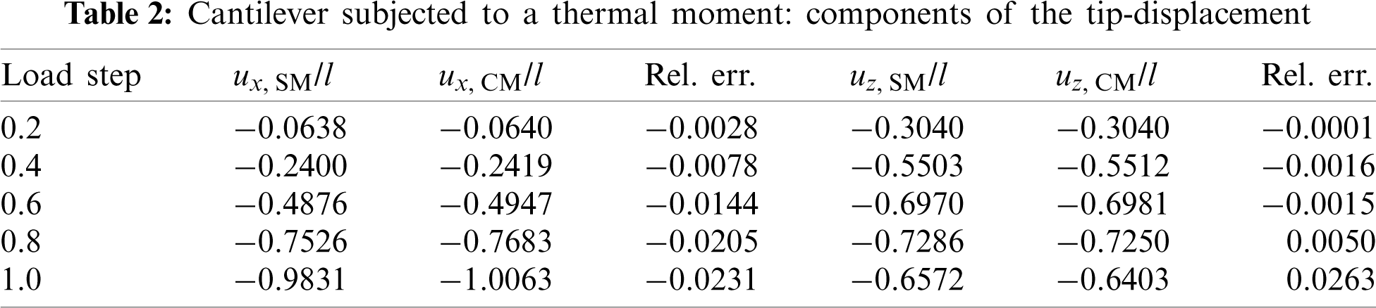
Figure 3: Cantilever subjected to a thermal moment: Comparison of the axial tip-displacement ux(x = l, y = 0, z = 0) (left) and transverse deflection uz(x = l, y = 0, z = 0) (right) obtained with the proposed structural mechanics formulation (SM) and the three-dimensional continuum mechanics (CM), respectively

Corresponding numerical values along with relative errors, which remain in the range of single-digit percentage, are given in Table 2. Note that the one-dimensional beam model has only 120 degrees of freedom, whereas the three-dimensional model requires 44640 degrees of freedom with constraints as well as symmetry conditions (uy(x, y = 0, z = 0)) already being accounted for and internal degrees of freedom being eliminated by means of static condensation.

Combined Thermo-Mechanical Loading

In a second example, we subject the cantilever to combined thermo-mechanical loading. For this purpose, a transverse tip-force Fext = −3YJy/l2 is applied first, before a (non-dimensional) thermal curvature kθ is gradually imposed. In the three-dimensional continuum mechanics setting, the tip-force is realized as a uniform surface traction t = tzez on the tip face (x = l), where tz = Fext/A. We assume a linear distribution of kθ along the beam’s axis, i.e.,

kθ=(1−xl)kθ(0).(79)

Within our study, the thermal load intensity is increased up to a value of

kθ(0)=−FextlhYJy,(80)

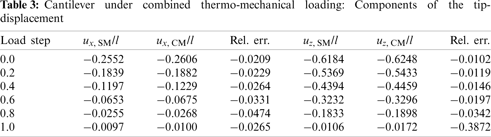
which, in the linear case, would exactly compensate the deflection by the tip-force, see, e.g., [40] for the related problem of ’shape control’ by means of piezoelectric actuation. Within the present non-linear setting, however, the beam’s deformation does not vanish exactly due to the non-linear distribution of thermal strains over the beam’s thickness, see Eq. (10). As opposed to our first example, shear deformation occurs under the mechanical loading by the transverse tip-force. Nonetheless, the results for the components of the (non-dimensional) tip-displacement obtained with the structural mechanics approach and the three-dimensional relations of continuum mechanics show excellent agreement, see Fig. 4, and the corresponding numerical values listed in Table 3.

Figure 4: Cantilever subjected to combined thermo-mechanical loading: Comparison of the axial tip-displacement ux(x = l, y = 0, z = 0) (left) and transverse deflection uz(x = l, y = 0, z = 0) (right) obtained with the proposed structural mechanics formulation (SM) and the three-dimensional continuum mechanics (CM), respectively

Conclusion

In the present contribution, our intent is to establish connections between various important isothermal and thermal continuum mechanics based constitutive formulations by Professor Karl S. Pister and his collaborators on the one hand side, and geometrically non-linear structural mechanics theories on the other side. While the latter offer important computational advantages, which are inherent in structural mechanics, the former continuum mechanics formulations rest upon firm thermodynamics based grounds. For continuum mechanics, we have particularly referred to a multiplicative decomposition for thermoelastic solids that was presented by Lu et al. [2], see Section 2 above. This decomposition allows a straight-forward extension of constitutive formulations associated with non-isothermal deformations to non-linear thermoelasticity, simply by replacing the (total) deformation gradient by its effective, stress-producing part. Assuming compressibility together with isotropy, the thermal extension of five isothermal hyperelastic constitutive relations from the literature, partly introduced or initiated in works of Karl Pister, have been discussed in Section 3. For structural mechanics, we have referred to the celebrated geometrically exact finite-strain theory by Reissner [8], in which constitutive relations, however, are to be stipulated on the structural level as relations stress resultants and generalized strains, which is in contrast to the continuum mechanics type stress-strain formulations. For isothermal problems, this gap was bridged by Irschik et al. [9 , 10], who utilized a non-linear stress-strain relation suggested, e.g., in the books by Wriggers [4] and Simo et al. [5], and which can be understood as a member of a class of isothermal constitutive relations introduced by Simo et al. [6], see also Hartmann [7]. Reissner’s beam theory and the contributions of Gerstmayr and Irschik have been summarized in Section 4 above. Eventually, we have presented consistent thermoelastic relations between stress resultants and generalized strains, which are computed from the thermal extension of the aforementioned isothermal stress-strain relation of the Simo-Pister type. Simple numerical examples show the efficacy of the proposed continuum mechanics-based extension of Reissner’s beam theory to thermo-mechanical problems. In the above formulations, we have also tried to present connections between the Austrian school of thermal stresses, which is formed by works of Ernst Milan, Heinz Parkus and Franz Ziegler, a school from which we stem, and important works of Professor Karl S. Pister, to whom the present contribution is dedicated on the occasion of his 95th birthday.

Funding Statement: The authors acknowledge the support by the Linz Center of Mechatronics (LCM) in the framework of the Austrian COMET-K2 program.

Conflicts of Interest: The authors declare that they have no conflicts of interest to report regarding the present study.

This work is licensed under a Creative Commons Attribution 4.0 International License, which permits unrestricted use, distribution, and reproduction in any medium, provided the original work is properly cited.