| Computer Modeling in Engineering & Sciences |
DOI: 10.32604/cmes.2021.017883
ARTICLE
A Meshless and Matrix-Free Approach to Modeling Turbulent Fluid Flow
Dedicated to Professor Karl Stark Pister for his 95th birthday
William Marsh Rice University, Houston, Texas, 77251-1892, USA
*Corresponding Author: Andrew Meade. Email: meade@rice.edu
Received: 14 June 2021; Accepted: 06 July 2021
Abstract: A meshless and matrix-free fluid dynamics solver (SOMA) is introduced that avoids the need for user generated and/or analyzed grids, volumes, and meshes. Incremental building of the approximation avoids creation and inversion of possibly dense block diagonal matrices and significantly reduces user interaction. Validation results are presented from the application of SOMA to subsonic, compressible, and turbulent flow over an adiabatic flat plate.
Keywords: Mesh free; Navier-stokes; turbulent flow; machine learning
The cost associated with Computational Fluid Dynamics (CFD) analysis has helped fuel the drive for programming methods that maximize the numerical data gathering capacity for a given level of computational effort and memory allocation. We believe that the Sequentially Optimized Meshfree Approximation (SOMA) method is another step in this direction [1,2].
SOMA is a meshless, volume-free, and matrix-free nonlinear differential equation solver. Flow simulations solvable by SOMA can be unsteady, compressible, and viscous. When flows are not solved purely steady state, SOMA has both explicit and implicit time stepping methods as well as the ability to switch dynamically between the two methods depending upon either computational efficiency or convergence criteria.
As a meshless method SOMA does not require Jacobians, information on mesh connectivity, or transformations between physical and computational domains through conformal maps. This simplifies the application of Adaptive Domain Refinement (ADR) techniques [3].
Other benefits and advancements associated with SOMA improve on both meshed and other meshless methods. Foremost among these, SOMA eliminates the need to invert large, possibly dense, block diagonal matrices in the solution of the governing equations. Solutions to the flow variables are determined through incrementally built approximations, and the governing equations can remain in vector form. Thus, SOMA eliminates the computational costs both of calculating and of inverting the system mass matrix.
The decades of analysis and work associated with other methods such as boundary element method (BEM), finite volume method (FVM) and finite difference method (FDM) with respect to numerical stability, upwinding, CFL number, characteristic lines, system eigenvalues, and many others can be directly applied to SOMA. This application can occur with little to no modification to account for the meshfree nature of SOMA. Additionally, boundary condition enforcement at farfield and surface locations can follow the methods used in FDM, FVM, and BEM [4], including extrapolation and ghost points. Finally, SOMA greatly reduces the required man-hours for domain discretization and adaptation, since there is no mesh to inspect and eliminates the need for user involvement during solution.
A general approximation to some true function u can be generated [5] using the n level weighted sum
where
In SOMA the approximations are built by holding the un−1 approximation fixed and optimizing the specific coefficient cn and basis function ϕn. The approximation can be written as
As there are no limitations on their distribution, a wide class of bases can be mixed and used (e.g., B-splines, radial basis functions, and low-order polynomials).
For a differential equation, say H is the system operator and f is the system forcing function. Then the solution approximation that SOMA generates will produce some error.
that can be reduced by growing the order j of the approximation. The residual of the previous differential equation at the nth stage becomes
Reformulating this as an optimization problem, the objective function can be written as
where 〈 ·,· 〉 can be the sum root of the squares (e.g., collocation method [6]) or the inner product (e.g., Method of Weighted Residuals [7]). The collocation method,
is used in this work, where np is the number of evaluation points. The construction of the weighted series progresses until ɛn ≤ ɛmax, where ɛmax is a user defined accuracy threshold.
3 Using SOMA-Radial Basis Functions
The basis function most often used in this work is the Gaussian Radial Basis Function (GRBF). The form for the ith basis is
where
However, capturing steep gradients in the dependent variable by simple smooth functions like GRBFs can be troublesome. To alleviate this difficulty, SOMA can augment the symmetric GRBF with an offset hyperbolic tangent function to create the “quasi-upwind” asymmetric Hyperbolic Radial Basis Functions (HRBF). These functions require additional parameters to determine the steepness of the asymmetry and its orientation but are also known analytically. The form for the ith basis function is
where
Eqs. (7) and (8) are the two forms of the basis function which SOMA uses to approximate the dependent variable. Examples of these two basis functions in two dimensions are shown in Fig. 1 for both contour and perspective views. It can be seen that the GRBFs are symmetric about the center while the HRBFs are steeper on one side. This steepness is controlled by the
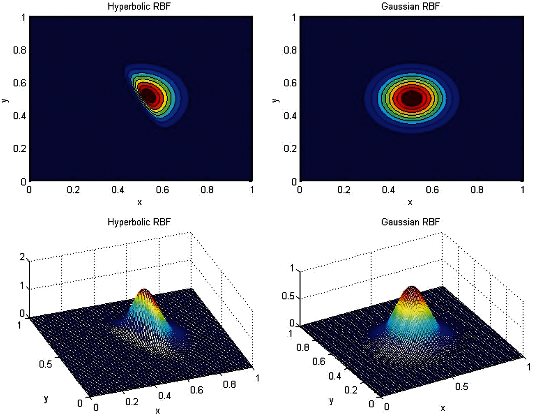
Figure 1: Examples of gaussian and hyperbolic radial basis functions
SOMA optimizes both HRBF and GRBF using a genetic algorithm (GA) [8]. When starting the optimization routine for a given iteration, the basis function parameters cn, ξc,n, βn,
When the governing equations are coupled and/or multi-variable non-linear equations (e.g., Navier-Stokes) all variables play a role in the value and the location of the maximum magnitude from all of the discrete residuals. Because each equation residual is primarily related to one of the flow variables, initializing its basis function center at that residual’s maximum magnitude tends to provide a good starting location. If the residuals are of similar magnitude, then randomly initializing the centers inside the convex hull of those values and bounding the search to within one or two radii of that hull also tends to greatly improve performance [2].
By default, GRBFs are used as they have fewer parameters to optimize. However, when a modeling problem requires too narrow a GRBF, SOMA switches to the HRBF form. We define a GRBF as too narrow when the radius encompasses fewer than five of the nearest evaluation points in two dimensions and nine points in three dimensions. The HRBF form is initialized as an asymmetric basis. Once the optimization routine no longer selects an asymmetric form (i.e.,
This section explains the means by which derivatives are numerically calculated, the means for upwinding convective flows, and the means for switching between explicit and implicit time marching.
To start, our flux vector formulation of the Navier-Stokes equations is defined in the traditional manner
with repeated indices indicating summation. Using the three-dimensional Cartesian velocity vector
we can write
for the conserved variables density (ρ), momentum flux (ρ Uc,i) and energy (E). We write
for the velocity magnitude,
for the ideal gas pressure, and
for the viscous shear stress, where δij is the Kronecker delta. We can now write
for the inviscid flux terms, and
for the viscous terms.
The working fluid in this work is considered to be air (specific heat ratio, γ = 1.4), thus temperature T can be defined through the ideal gas law and the dynamic viscosity (μ) using Sutherland’s Law. Dependent and independent variables were non-dimensionalized by farfield conditions ρ∞ and U∞ and the appropriate characteristic length L similar to the method in [9].
The normalized forms of energy and pressure used by SOMA were constructed such that they were unity at the farfield with a coefficient, i.e.,
where M∞ is the farfield Mach number. While this has no effect on the equations themselves, it reduces the optimization search space to a near unit hypercube, which has been shown to improve performance of SOMA in tests.
If we define the equation residuals for the mass, momentum, and energy equations as Rρ, RUc,j, and RE, respectively, then the objective function for the Navier-Stokes validation problems is written as
where
for ψ = ρ, Uc , E. Note that
Dirichlet boundary conditions are upheld directly by
Neumann or mixed conditions are enforced by using ghost points,
along the boundary γN. Fig. 2, duplicated from reference [10], shows an illustration of ghost points at a boundary. Both of these methods can be combined to enforce Cauchy boundary conditions easily.
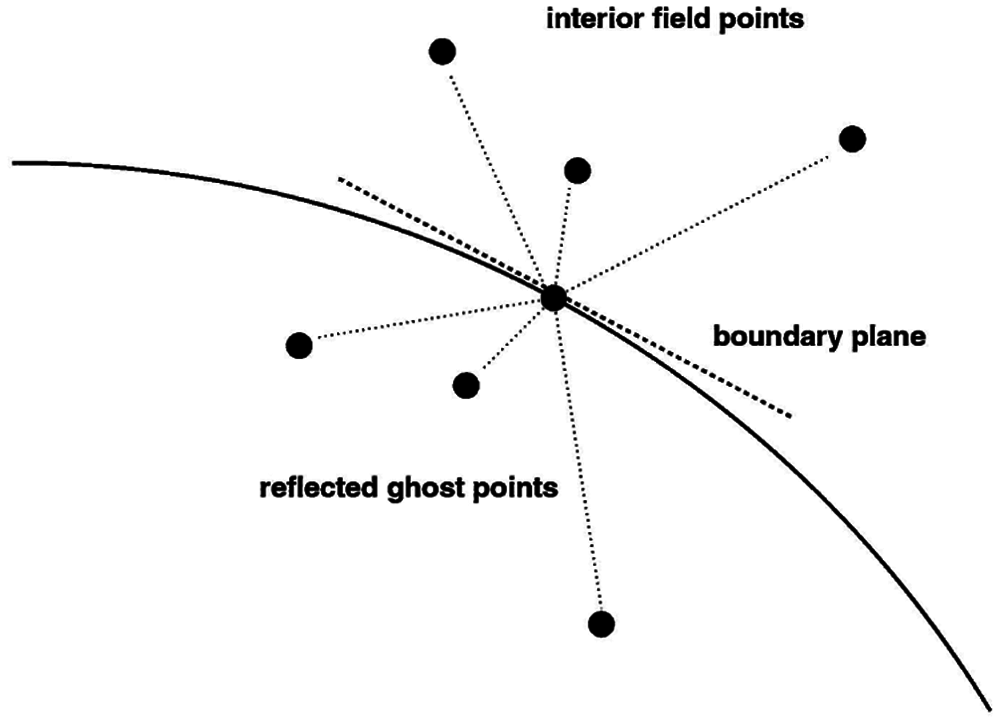
Figure 2: Ghost and real evaluation points at surface boundary [10]
For the special case of tangent/slip wall velocity (e.g., Euler flow), a few extra steps are necessary. First, SOMA must convert the velocity vector from global Cartesian to the surface Normal-Tangential-Binormal coordinate frame velocity vector. We use a rotation matrix Rs,c which converts from Cartesian coordinates to Surface Normal-Tangential-Binormal coordinates. The required velocity vector is
at each point along the surface boundary ΓS. The tangential/slip velocity boundary condition is enforced by setting
and the Cartesian velocity vector at the ghost points is calculated by inverting the rotation matrix Rs,c against the Normal-Tangential-Binormal coordinate ghost velocity vector. Through the use of upwind techniques conditions can also be applied to arbitrary geometries.
Differential Quadrature (DQ) is used as the method for numerically calculating derivatives in this work. While it might seem that DQ would add extra computational cost to SOMA versus using exact function derivatives, it alleviates some of the major cost and difficulty associated with implementing boundary conditions on irregular geometries.
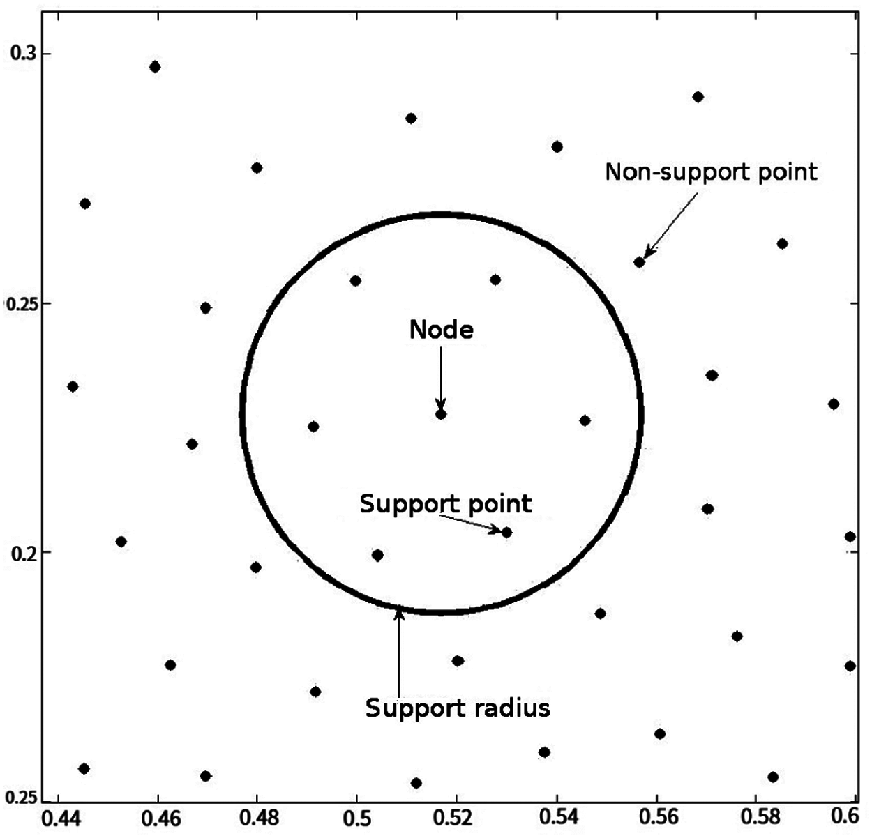
Figure 3: Example of a differential quadrature cloud
In this work the “node” is the point of interest and the remaining subset is referred to as “support points” or “supports”. Fig. 3 illustrates an example of a node, support, and subset, also known as the support “cloud,” for a general unstructured mesh. The subset usually consists of all points within some radius of the node [11]. We can then approximate the mth x-derivative at the node
where the node as a support point is included. The same formulation is used for derivatives of y and z where the DQ coefficients are wy,mij and wz,mij, respectively. For an lth y cross derivative, wx,m−l,y,lij.
Using a single independent variable as an example, the DQ weighting coefficients are determined using the known data from the basis functions. The function u(x) is a linear combination of the basis functions ϕ(xi,xc,k) and Eq. (23) is a linear operator. Therefore, if the basis functions satisfy Eq. (23), then it is guaranteed that u(x) must also satisfy this equation [12,13]. Differential quadrature is then applied to the basis functions, which yields
where ϕk(x) is used to denote the k-th basis function, i.e., the basis function centered at xc,k. If Eq. (24) is rewritten as a matrix equation, then the weighting coefficients can be determined by
where
and Ax is the matrix of x-derivatives of the basis functions,
While it is possible to calculate higher order and cross derivatives with DQ, it is frequently more effective to calculate only first derivatives for the flow variables, combine them into flux vectors, and then calculate the derivatives of those. For example, with the three-dimensional Navier-Stokes equations, SOMA would need to calculate the first, second, and cross derivatives for all flow variables in all directions. For nq quadrature points in a domain of dimension D, calculating all these derivatives requires O((D + 2) * (D + 2 + 2D−1 − 1) * nq * np) operations while the flux formulation requires only O((D + 2) * D * nq * nq * np) operations.
While typically nq is greater than 3, it is usually fewer than 20 meaning that in three dimensions the formulations are off by less than a factor of 7, and the extra work is offset by two major bonuses associated with the flux forms. First, there are fewer operations as there are fewer terms to multiply, and second, the flux forms are usually smoother than the primitive variables themselves [14]. Because all numerical derivative calculations involve some error, having smoother functions reduces the absolute magnitude of this error thus improving the accuracy of the method. We determined that the increase in accuracy of the flux formulation was worth the modest amount of extra DQ work.
In SOMA, DQ uses the Roe approximate third order solver [14] modified through the van Albada limiting routine [15] because of its meshfree nature. Application of the CUSP scheme [16] reduces computation time without drastically reducing accuracy.
Time marching techniques were used for the validation problems solved by SOMA even in cases which were physically at steady state. In these steady cases time marching will be referred to as false-transient methods. In all validation problems the two techniques available for time integration are explicit and implicit.
For explicit time (t) marching, SOMA uses the fourth order Runge-Kutta (RK4) method [17]. This method is implemented as follows:
Advantages of this Runge-Kutta method over the simple explicit Euler method [18] include a time accuracy of O(∆t4) compared to O(∆t) and a larger stable time step according to the relation
Even accounting for the multi-step process of Runge-Kutta techniques, explicit methods are much less computationally expensive than implicit methods, but they also have the drawback of much smaller stable time steps. If the time step is bound by conditions other than stability (e.g., aliasing of periodic flows or turbulent eddy time scales) then explicit time integration can be the more efficient method. However, implicit methods are far more computationally expedient, especially in steady-state problems.
In its most basic form, the implicit Euler method [18] can be written as
Because the updated flow variable is in both the unsteady and the nonlinear flux vector, the flux Jacobians [19] from the Roe upwind method are used to linearize the equations.
Unlike these traditional methods there is no need for the inversion of matrices in SOMA which can be computationally expensive for three-dimensional external flows. With SOMA, the dependent variables are initialized as
An adaptive and local time step is applied in this work which gives the largest stable step possible for any given set of flow conditions. In the three-dimensional case, using the standard Courant-Friedrichs-Lewy parameter (CFL), the step is calculated as
with
from the Prandtl number (Pr) and Reynolds number (Re), where
and
are the inviscid and viscous eigenterms, respectively, of the system. We define aj as the acoustic speed at location j. In cases where a local time step is not feasible, the smallest of the possible local time steps would be used for the whole domain.
The inversion of a roughly sparse matrix with ne equations or dependent variables is
4.3.4 Explicit/Implicit Switch
SOMA typically solves the flow equations using an implicit formulation allowing for larger time steps and quick conversion to steady state or to stable periodic flows (e.g., vortex shedding). There are, however, times when it is necessary to switch to an explicit solver even in the middle of a simulation run. Because implicit methods are far more computationally expensive than explicit methods, it is necessary to take time steps large enough to account for the difference in computational wall clock time. In this work we have used ∆timplicit,i = 95 ∆texplicit,i.
If the optimization of ɛ cannot drop below the tolerance ɛmax when using the implicit formulation, the weighted series that was developed for the current time step is discarded. Initializing with the known solution from the previous time step, SOMA time marches explicitly until it has advanced the equivalent of one implicit time step. At this point the solver switches back to an implicit method and advances.
For a k − ω model, the stress term is defined as
and the heat flux term as
where μt and κt are the turbulent dynamic viscosity and thermal conductivity, respectively. Using the normalization described in Section 4, the heat flux can be rewritten as
where Prt is the turbulent Prandtl number.
In this work, we utilized the Menter single shear-stress-transport (SST) k − ω model. Full details of the Menter-SST model, including values of constants, can be found in reference [21]. The governing equation for k is presented here as
and the governing equation for ω
With k and ω determined, the turbulent viscosity can be calculated from
which allows for time advancement of the remaining Navier-Stokes equations. Strong coupling of the SST model to the mass, momentum, and energy equations is straightforward.
For validation of the solution method, we chose relevant numerical problems of increasing complexity. SOMA was first used to approximate the solution to the steady state convective-diffusion equation (Burger’s equation) to test the method’s stability and convergence rate. Then SOMA was used to model vortex shedding about a circular cylinder (incompressible time-accurate Navier-Stokes equations) and on to inviscid, compressible flow past an NACA 0012 airfoil and ONERA M6 wing at angle of attack (compressible false-transient two- and three-dimensional Euler equations). Finally, SOMA was used to model the subsonic compressible turbulent flow over an adiabatic flat plate with zero pressure gradient. For the turbulence problem comparison data were taken from the NASA Langley Research Center flow verification website [22], including the domain discretization, shown in Fig. 4. The value ɛmax was set to 1 × 10⁻⁷ for all results. The simulations were run in serial using a single-core Intel i5 processor. SOMA generally runs 10% slower on the validation problems as compared to our FVM solvers.
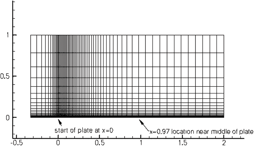
Figure 4: Problem domain and nodes from [22]
6.1 Results for Convection-Diffusion
In this paper, the stationary convection-diffusion equation modeling a boundary layer also serves to evaluate the convergence of SOMA with increasing values of np. The second order linear differential equation is given by
where λ and ν are the convective viscosity and diffusion coefficients, respectively. The solution to Eq. (41) can be written as
For our validation, the Reynolds number was set to 20 and SOMA was run up to np = 300 with points uniformly distributed within the problem domain. The GRBF was utilized with three separate optimization routines: Fmincon, a pattern search method, and a GA [8]. For this convergence study, SOMA was run 50 times and the results averaged. Fig. 5 shows the log of averaged RMS of the error vs. the log of np. The GA and pattern search give quintic convergence for the initial 20–50 GRBFs, then a linear convergence rate. The results for Fmincon are significantly worse both in terms of convergence and overall accuracy. Consequently, the GA was used in the remaining validation cases. It should be noted that all of the SOMA solutions for this case were stable for Re = 20.
6.2 Results for Flow Past a Cylinder
Inlet conditions for this validation case were M∞ = 0.5 and Re = 300. The surface geometry was a circular cylinder of radius r = 0.5 centered at the origin. SOMA used np = 8,349 points. A comparison of the results is given in the form of time histories of the coefficients for both SOMA and reference [24]. As shown in Fig. 6, periodic unsteady values for the lift and drag coefficients (cl and cd) match well with the comparison data.
6.3 Results for Inviscid Compressible Flow Past an Airfoil
For this validation case the conditions used were angle of incidence
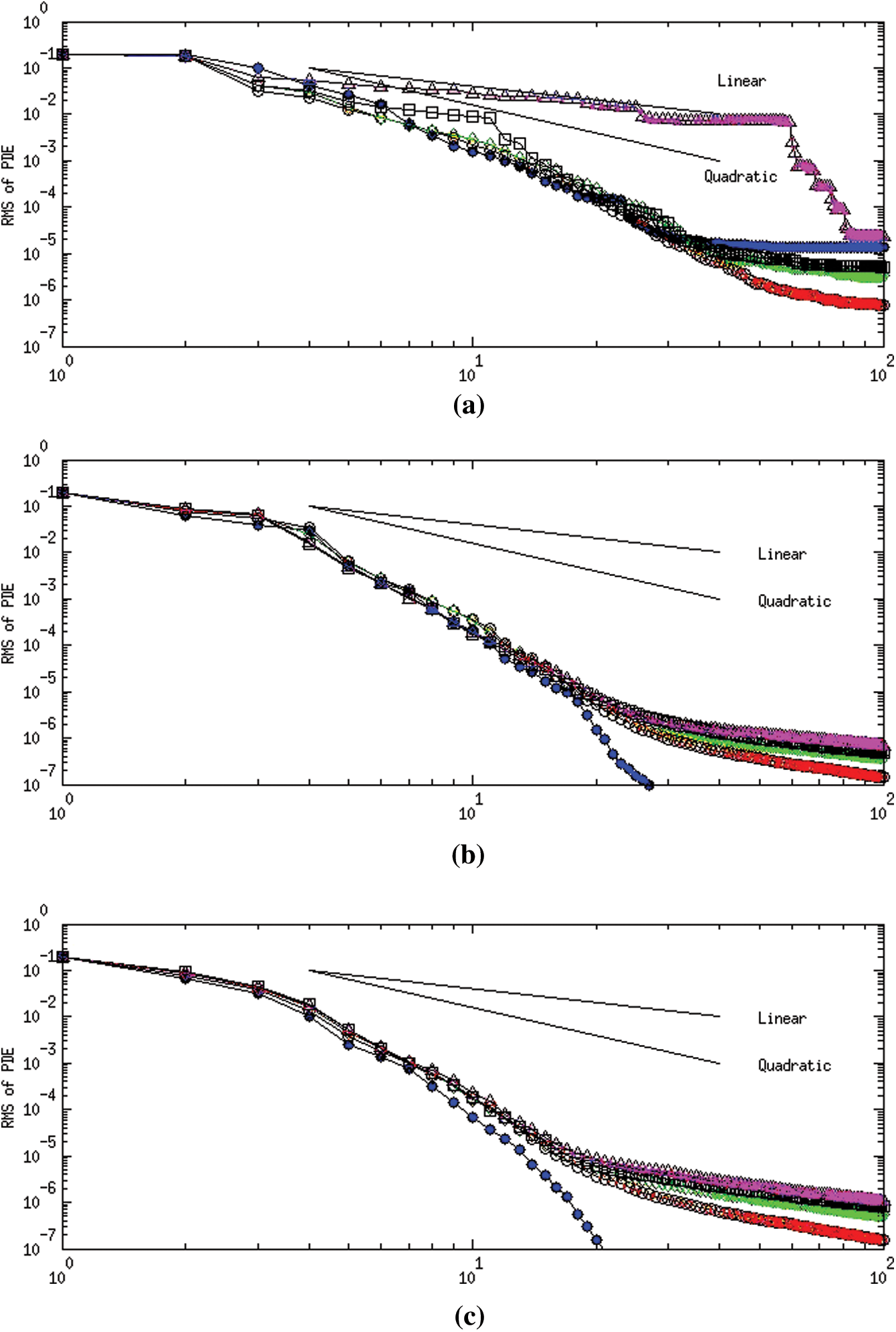
Figure 5: Rate of convergence-convection-diffusion equation with Re = 20. (a) Fmincon (b) Pattern search (c) Genetic algorithm
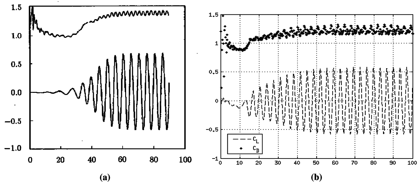
Figure 6: Time history of the circular cylinder’s lift and drag coefficients. (a) Reference [24] (b) SOMA
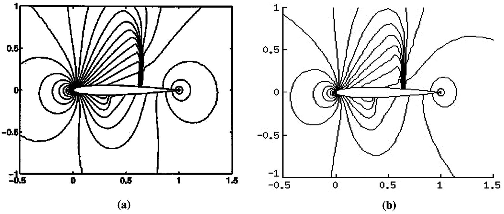
Figure 7: NACA 0012 mach contours. (a) Finite volume [25] (b) SOMA
6.4 Results for Inviscid Compressible Flow Past a Swept Wing
For this validation case the conditions used were
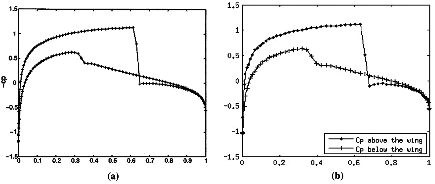
Figure 8: NACA 0012 surface pressure coefficient distribution along the normalized chord (x/c). (a) Finite volume [25] (b) SOMA
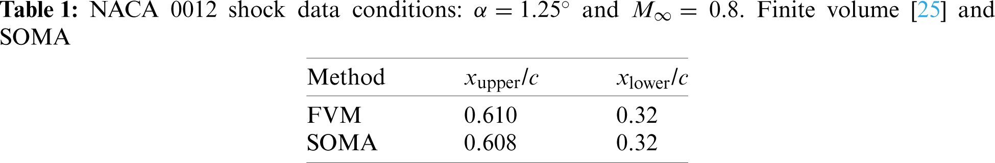
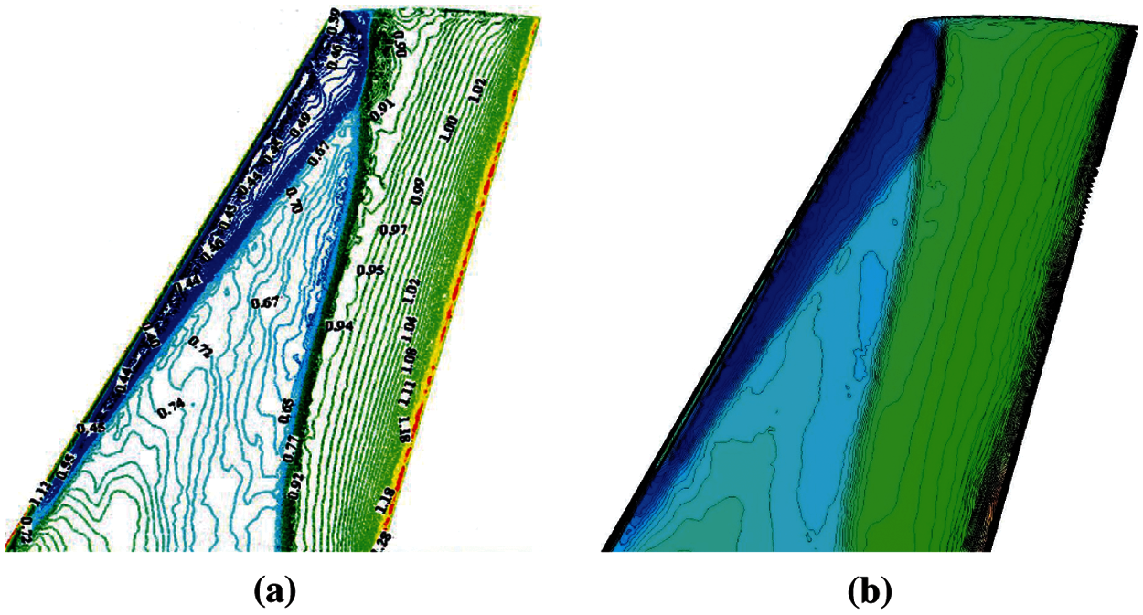
Figure 9: ONERA M6 wing surface CP contours. (a) Unstructured FEM [27], (b) SOMA
In order to show the level of quantitative agreement, chord-wise distributions of the surface CP about the upper (U) and lower (L) surfaces of the wing are compared at span-wise locations z/b = 0.65 and z/b = 0.80. Results from a SOMA simulation are shown in Fig. 10 alongside the CP data from reference [26] and from a structured finite volume (STAR) simulation [1]. These figures show general agreement with the AGARD 138 data at both span-wise locations. However, both methods also show over- and under-shoots at x/c locations. At the z/b = 0.80 location both methods missed the middle ridge. Reference [26] notes that even computer codes that included viscosity in their approximation missed the middle ridge.
Figure 10: Comparison of inviscid CP along ONERA M6 wing. (a) z/b = 0.65, (b) z/b = 0.80
6.5 Results for Turbulent Flow over a Flat Plate
The inflow conditions for the turbulent flow over a flat plate were
Results from the NASA test case were given using a 545 × 385 grid (equivalent to np = 209,825). With the convergence of SOMA demonstrated in Section 6.1, the code ran on a domain of only np = 52,689 to demonstrate that SOMA can recover accurate results with a sparser discretization than reference [22]. To facilitate comparison, results from both SOMA and the NASA solver were plotted on an x, y grid in Matlab using the same normalizations, contours, and coloring schemes found in reference [22]. Fig. 11 shows the turbulent kinetic energy
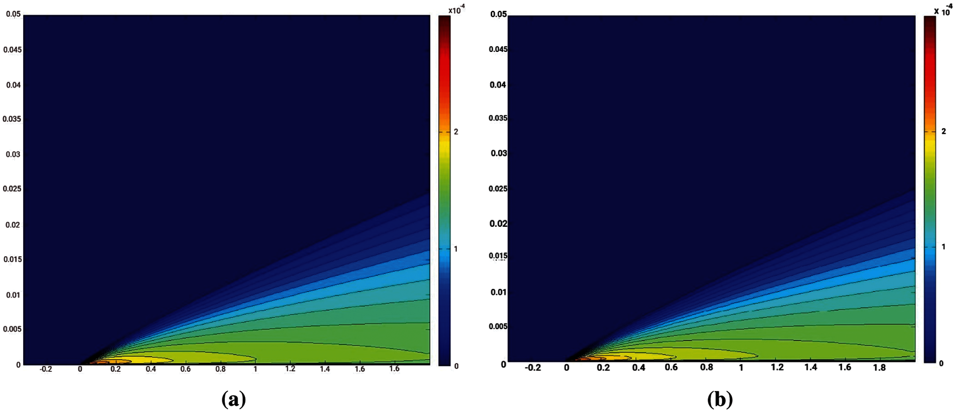
Figure 11: Turbulent kinetic energy,
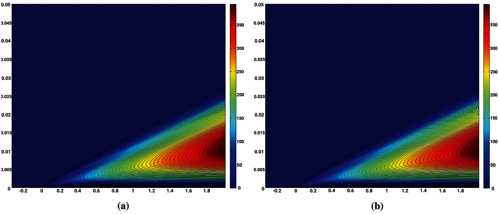
Figure 12: Turbulent viscosity, μt/μ∞. (a) Reference [22], (b) SOMA
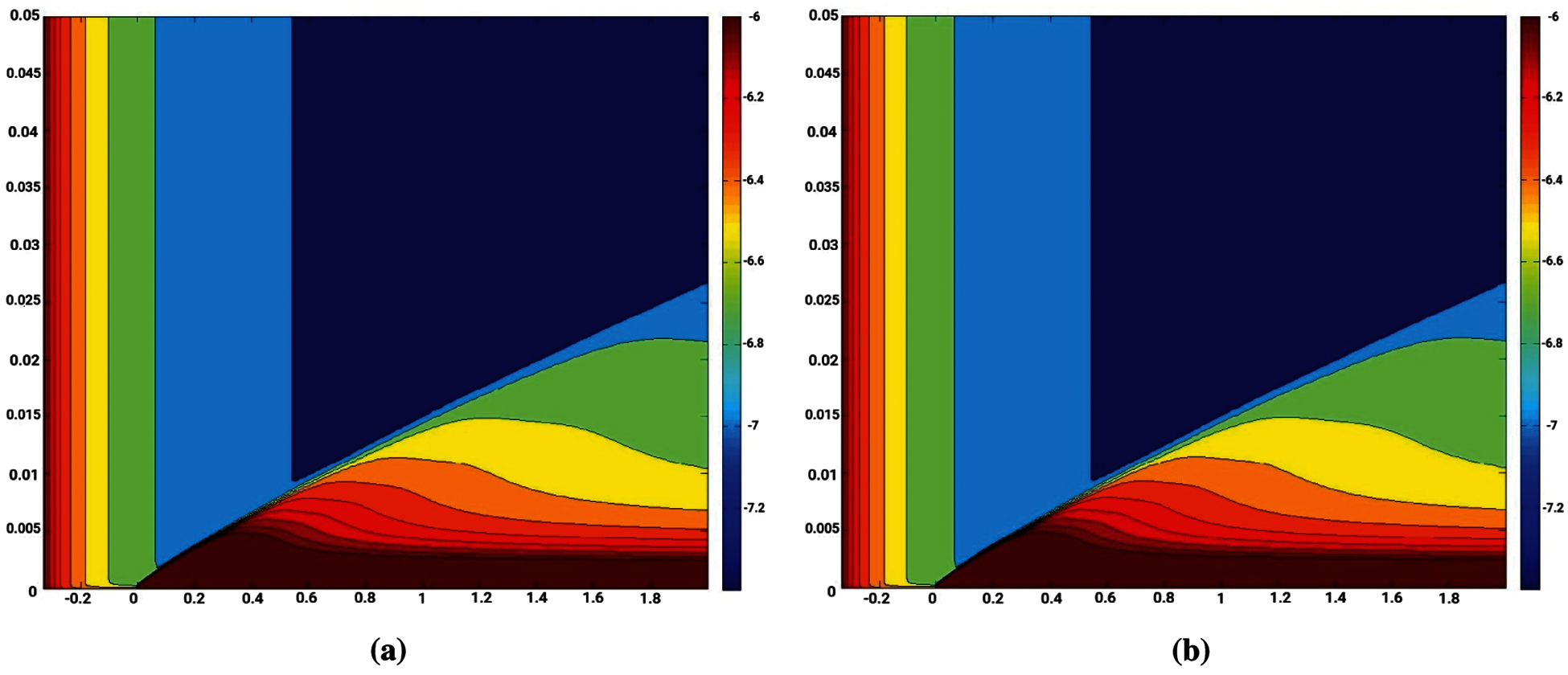
Figure 13: Turbulent eddy frequency,
Conventional techniques in numerical modeling can still require significant man hours for grid generation along with the need to invert large, sometimes dense, block diagonal matrices. With significant reduction in user interaction time the Sequentially Optimized Meshfree Approximation (SOMA) method serves as a new computational fluid dynamics solver eliminating the need for the previously mentioned matrices.
Unlike conventional techniques that require grids or volumes along with the corresponding connectivity data, SOMA only requires the coordinates of the evaluation points to model the flow. SOMA approximates the dependent variables incrementally through a greedy algorithm and minimization of the scalar form of the governing equations. As a result, the derivation and inversion of a condensed “mass” matrix are unnecessary. Reduction in the amount of user interaction time allows SOMA to improve as computing power continues to increase.
Although the three-dimensional validation case was restricted to the Euler equations, SOMA has been successfully applied to three-dimensional compressible laminar flow problems [1,2]. Since additional flow variables can significantly enlarge the optimization search space, improvements to the sequential optimization routine will be needed to handle a three-dimensional turbulence model. A possible solution for future work will be the investigation of massively parallel pattern search methods supported by parallel processing hardware.
Acknowledgement: The authors wish to express their appreciation to the reviewers for their helpful suggestions which greatly improved the presentation of this paper.
Funding Statement: The authors received no specific funding for this study.
Conflicts of Interest: The authors declare that they have no conflicts of interest to report regarding the present study.
1. Wilkinson, M. (2012). Sequentially optimized meshfree approximation method as a new computational fluid dynamics solver (Ph.D. Thesis). Rice University, Houston, Texas. [Google Scholar]
2. Villarreal, J. (2021). Development of a meshfree and matrix-free method for compressible computational fluid dynamics (Ph.D. Thesis). Rice University, Houston, Texas. [Google Scholar]
3. Plewa, T., Linde, T., Weirs, V. G. (2005). Adaptive mesh refinement-theory and applications. Proceedings of the Chicago Workshop on Adaptive Mesh Refinement Methods, New York, Springer. [Google Scholar]
4. Gao, X. W. (2007). Explicit formulations for evaluation of velocity gradients using boundary-domain integral equations in 2D and 3D viscous flows. International Journal for Numerical Methods in Fluids, 54, 1351–1368. DOI 10.1002/(ISSN)1097-0363. [Google Scholar] [CrossRef]
5. Young, N. Y. (1988). Model order reduction: Theory, research aspects and applications. Cambridge, UK: Cambridge University Press. [Google Scholar]
6. Fletcher, C. A. J. (1984). Computational galerkin methods. Berlin, Germany: Springer-Verlag. [Google Scholar]
7. Finlayson, B. A. (1972). The method of weighted residuals and variational principles. Cambridge, Massachusetts, USA: Academic Press. [Google Scholar]
8. MathWorks documentation center (2014). Global optimization toolbox. Natick, Massachusetts, USA: The MathWorks Inc. [Google Scholar]
9. Hoffman, K. A., Chiang, S. T. (1993Computational fluid dynamics for engineers, vol. 1. Wichita, KS: Engineering Education System. [Google Scholar]
10. Katz, A., Jameson, A. (2010). Meshless scheme based on alignment constraints. AIAA Journal, 48(11), 2501–2511. DOI 10.2514/1.J050127. [Google Scholar] [CrossRef]
11. Shu, C., Ding, H., Yeo, K. S. (2005). Computation of incompressible navier-stokes equations by local RBF-based differential quadrature method. Computer Modeling in Engineering & Sciences, 7(2), 195–205. DOI 10.3970/cmes.2005.007.195. [Google Scholar] [CrossRef]
12. Shu, C. (2000). Differential quadrature and its application in engineering. Berlin, Germany: Springer. [Google Scholar]
13. Shen, Q. Z. (2010). Local rbf-based differential quadrature collocation method for the boundary layer problems. Engineering Analysis with Boundary Elements, 34(3), 213–228. DOI 10.1016/j.enganabound.2009. 10.004. [Google Scholar]
14. Anderson, J. D. (1995). Computational fluid dynamics: The basics with applications. New York, USA: McGraw-Hill. [Google Scholar]
15. Hirsch, C. (1988Numerical computation of internal and external flows, vol. 2, Hoboken, New Jersey, USA: Wiley. [Google Scholar]
16. Jameson, A. (1995). Analysis and design of numerical schemes for gas dynamics, 1: Artificial diffusion, upwind biasing, limiters and their effect on multigrid convergence. International Journal of Computational Fluid Dynamics, 4(3–4), 171–218. DOI 10.1080/10618569508904524. [Google Scholar] [CrossRef]
17. Chung, T. J. (2002). Computational fluid dynamics. Cambridge, UK: Cambridge University Press. [Google Scholar]
18. Ferziger, J. H., Peric, M. (1999). Computational methods for fluid dynamics. Berlin, Germany: Springer-Verlag. [Google Scholar]
19. Peyret, R., Taylor, T. D. (1983). Computational methods for fluid flow. Berlin, Germany: Springer-Verlag. [Google Scholar]
20. Ran, R. S., Huang, T. Z. (2006). The inverses of block tridiagonal matrices. Applied and Computational Mathematics, 179, 243–247. DOI 10.1016/j.amc.2005.11.098. [Google Scholar] [CrossRef]
21. Menter, F. (1994). Two-equation eddy-viscosity turbulence models for engineering applications. AIAA Journal, 32(8), 1598–1605. DOI 10.2514/3.12149. [Google Scholar] [CrossRef]
22. Rumsey, C. (2013). Langley research center turbulence modeling resource. http://turbmodels.larc.nasa.gov/flatplate.html/. [Google Scholar]
23. Fletcher, C. A. J. (1988). Computational techniques for fluid dynamics, vol. 1. Berlin, Germany: Springer-Verlag. [Google Scholar]
24. Xiaogang, D., Fenggan, Z. (2002). A novel slightly compressible model for low mach number perfect gas flow calculation. Acta Mechanica Sinica, 18(3), 193–208. DOI 10.1007/BF02487948. [Google Scholar] [CrossRef]
25. Buuren, R. V., Kuerten, J. G. M., Geurts, B. J. (1997). Instabilities of stationary inviscid compressible flow around an airfoil. Journal of Computational Physics, 138(2), 520–539. DOI 10.1006/jcph.1997.5830. [Google Scholar] [CrossRef]
26. Schmitt, V., Charpin, F. (1979). AGARD advisory report no. 138: Experimental data base for computer program assessment. https://ftp://ftp.rta.nato.int//PubFullText/AGARD/AR/AGARD-AR-138/AGARD-AR-138.pdf. [Google Scholar]
27. Manzari, M. T. (2005). Inviscid compressible flow computations on 3D unstructured grids. Scientia Iranica, 12(2), 207–216. http://scientiairanica.sharif.edu/article_2484.html. [Google Scholar]
 | This work is licensed under a Creative Commons Attribution 4.0 International License, which permits unrestricted use, distribution, and reproduction in any medium, provided the original work is properly cited. |