Computer Modeling in Engineering & Sciences

DOI: 10.32604/cmes.2021.017740

ARTICLE

Fluid and Osmotic Pressure Balance and Volume Stabilization in Cells

Dedicated to Professor Karl Stark Pister for his 95th birthday

Peter M. Pinsky*

Department of Mechanical Engineering, Stanford University, Stanford, 94305, CA, USA
*Corresponding Author: Peter M. Pinsky. Email: pinsky@stanford.edu
Received: 02 June 2021; Accepted: 26 July 2021

1  Introduction

A cell must concentrate and protect within its interior substances that are essential for its function—DNA, proteins, amino acids and sugars. These sequestered substances, which are entrapped within the cell, introduce a special challenge for the cell. They carry significant concentrations of charge that establishes a high osmotic pressure within the cell. The osmotic pressure difference between the intracellular and extracellular media produces a tendency to swelling by water inflow across the cell membrane. Such swelling can be arrested by two processes: actively reducing the cellular ionic content through ion pumps, and by the generation of internal fluid pressure that can act to stop the flow of water. In fact, both processes will act simultaneously. However, animal cells have fragile membranes and it has generally been accepted that the primary action of the pump-leak mechanism (PLM) is the active reduction of cellular ionic content and the concomitant reduction in osmotic pressure. As a result, models that have been developed to explain the PLM have concentrated on osmotic stabilization due to ion pumping [1–5]. The role of cellular fluid pressure, generated by the resistance to expansion of the cell membrane–cortex has received less attention [6–8]. A general framework for modeling the PLM including the role of fluid pressure is proposed in this work.

The movement of ions across the cell membrane occurs passively and actively. Passive transport occurs by diffusion and convection and requires no energy input. Active transport processes move ions against concentration gradients through the expenditure of energy. Both processes are important and the interplay between them, controlled by feedback [9], facilitates the regulation of cell volume, preventing potential cell rupture or collapse under changing conditions.

The cytoplasm (i.e., intracellular fluid) contains charged macromolecules and metabolites that are confined to the cell interior by entrapment and are impermeant with respect to the cell membrane—all such impermeant charged macromolecules will be referred to as fixed charges for brevity. The fixed charges localize mobile ions which form an electrical double layer of counterions and coions that screens the electric field. The resulting ion concentrations establish the osmotic pressure within the cell. If the extracellular solution has, for example, lower ionic concentrations, water will flow across the cell membrane and into the cell by osmosis, causing the cell to swell. It is the fixed charges that are essentially responsible for the swelling tendency of the cell. Active ion transporters (e.g., the Na+ ion pump) that convert energy from various sources, including adenosine triphosphate (ATP), are located in the cell membrane and produce outward and inward fluxes of ions that modulate the osmotic and fluid pressures to arrest and reverse cellular swelling [10].

The linear theory of nonequilibrium thermodynamics has been widely employed to model passive transport processes. The approach asserts the existence of a dissipation function which describes the rate of change of entropy production. It is expressed as the sum of a set of flux and conjugate (driving) force products. For example, the classical study of Kedem et al. [11,12] used this approach to obtain the flux definitions that are conjugate to the fluid and osmotic pressures for a non-electrolyte solution. Then, considering near-equilibrium, a linear relationship between each flux and all conjugate forces is postulated. The result is a set of phenomenological equations that describes all interactions between the solvent and solutes and which is expressed with transport coefficients that have the significant merit of being amenable to experimental measurement.

When the solutes crossing the membrane are charged, the nonequilibrium thermodynamic description is more challenging and the system exhibits new features. A very general framework based on linear nonequilibrium thermodynamics has been given by Kedem et al. [13] and includes many electrokinetic phenomena within its scope. More recently, Li [14] proposed phenomenological equations for the passive transport of ionic solutions that account for electrostatic interactions between ions. This was extended by Cheng et al. [15] to account for fixed charges associated with proteoglycans for application to the corneal endothelium. The latter work identified a fluid pressure component that appears during active ion pumping and which must be considered in the balance of fluid and osmotic pressure. The goal of the present paper is to describe the temporal and steady state behavior of the pump-leak system utilizing the fully general framework of nonequilibrium thermodynamics.

We start with a brief review of the development of phenomenological equations for passive transport across a semipermeable membrane separating two ionic solutions, one of which contains impermeant charged macromolecules. Extension of the theory for active ion transport is then described, including derivation of the generalized pressure conjugate to the active ion flux. Analytical steady state solutions are obtained for both the passive and active cases and considering an intracellular binary electrolyte solution. Solutions to the temporal problem are obtained numerically.

To illustrate the scope and features of the theory, a numerical study of a highly idealized model of a human cell is introduced. The cell is in suspension (without attachments) and is subjected to a sequence of hypotonic and hypertonic shocks. For simplicity, the intracellular and extracellular solutions are taken to be binary electrolyte solutions and the phenomenological equations are suitably specialized. The model is first applied to analyzing the response of the cell model with only passive transport. In a second analysis, active cation transport is initiated when a signal based on membrane tension is received. This simulation provides the time course of the cell radius, fluid pressure, osmotic pressures, and other quantities. The numerical results suggest that the model replicates the essential features of the PLM and that the fluid pressure component arising from the active ion flux is an essential factor in the balance of fluid and osmotic pressures, including under steady state conditions.

2  Modified Kedem-Katchalsky Equations for Passive Transport

The Kedem and Katchalsky (KK) phenomenological equations [11–12,16,17] are based on nonequilibrium thermodynamics and describe the transport of water and solutes across a semipermeable membrane separating two non-electrolyte solutions. They take the form

Jv=Lp(ΔP−∑k=1NspeciesσkRTΔCk)(1)

and

Jk=(1−σk)C¯kJv+ωkRTΔCk(2)

where Jv is the volume flow and Jk is the solute molar flux. In (1), ΔP and Δ Ck are the fluid pressure and solute concentration differences across the membrane, respectively, Lp is the hydraulic conductivity, σ k is the reflection coefficient for species k, R is the gas constant and T is the temperature. In (2), C¯k is the mean value of the solute concentration across the membrane, and ω k is the solute permeability. These equations have found remarkably wide application in practise because the transport parameters are readily amenable to experimental measurement.

For electrolyte solutions, the transport equations should account for the electrostatic effects of the fixed and mobile ion charges. The procedure to obtain suitable modified KK phenomenological equations [14,15] is briefly reviewed as follows. The chemical potential of water with mole fraction Xw is μ w = ν wP + RTlnXw, where νw is the partial volume of the water and P is the fluid pressure. For dilute solutions, μ w may be equivalently expressed in terms of the ion concentrations Ck as

μw=νw(P−RT∑k=1NspeciesCk)(3)

where Nspecies is the number of ion species. For brevity, sums over all ionic species will henceforward be indicated as ∑. For ionic solutes, the electrochemical potential of species k is

μk=νkP+RTln⁡Ck+zkFψ(4)

where ν k is the partial volume of the ion, zk is the valence number, F is the Faraday constant and ψ is the electrostatic potential.

With reference to a biological cell, ion concentrations in the intracellular fluid are denoted Ck and in the extracellular fluid Ck0 and membrane differences are defined to be ΔCk=Ck−Ck0. For water Δμw=μwin−μwout and therefore, from (3),

Δμw=νw(ΔP−RT∑ΔCk)(5)

where ΔP = Pin − Pout is the membrane fluid pressure difference. Similarly, Δμk=μkin−μkout and therefore, from (4),

Δμk=νkΔP+RTln⁡(CkCk0)+zkFΔψ(6)

where Δ ψ = ψ in − ψ out is the membrane potential difference. We will use the linearized form1 of (6)

Δμk=νkΔP+RTΔCkC¯k+ziFΔψ(7)

where is the average ionic concentration through the membrane.

The dissipation function Φ, which measures the rate of entropy production for irreversible processes, is expressed as [11,12]

Φ=JwΔμw+∑JkΔμk(8)

where Jw and Jk are the water and ion molar fluxes, respectively, and where Δμ w and Δμ k are their conjugate driving forces. Instead of Jw and Jk, we seek the forces conjugate to the more readily measurable volume flow Jv and ion exchange flux JDk defined by

Jv=νwJw+∑νkJk(9)

and

JDk=JkC¯k−JwCw(10)

The ion exchange flux JDk may be interpreted as the velocity of ion k relative to the solvent. By direct manipulation of (8), it may be shown [15] that

Φ=JvXv+∑JDkXk(11)

where the conjugate forces Xv and Xs are given by

Xv=ΔP+RT(1−νwCw)∑ΔCk+∑zkC¯kFΔψ(12)

and

Xs=RTΔCs+zsC¯sFΔψ−νsC¯s(RT(1−νwCw)∑ΔCk+∑zkC¯kFΔψ),s=1,2,…,Nspecies(13)

By assuming a dilute solution such that νk<< 1 and νwCw≈1, (12) and (13) reduce to

Xv=ΔP+∑zkC¯kFΔψ(14)

and

Xk=RTΔCk+zkC¯kFΔψ(15)

The flows defined in (9) and (10) are now expressed as phenomenological equations having the form

Jv=LpXv−Lp∑σkXk(16)

JDs=−LpσsXv+∑LDskXk,(17)

where Lp is the hydraulic conductivity and σ k is the reflection coefficient of species k. LDsk are permeability coefficients which satisfy the Onsager reciprocal relation such that LDsk = LDks, reducing the number of independent coefficients.

Under the assumption of a dilute solution we have Js=Cs(Jv+JDs) which, after introducing (16) and (17), results in [15]

Js=(1−σs)C¯sJv+∑ωskXk,s=1,2,…,Nspecies(18)

where the solute permeability coefficient ωsk=C¯s(LDsk−Lpσsσk). Ignoring interactions between ions such that ω sk = 0 for s ≠ k and replacing ω ss with ω s reduces (18) to

Js=(1−σs)C¯sJv+ωsXs,s=1,2,…,Nspecies(19)

with ωs=C¯s(LDss−Lpσs2) Finally, employing (14) and (15) in (16) gives the volume flux

Jv=Lp(ΔP−∑[σkRTΔCk−(1−σk)zkC¯kFΔψ])(20)

and likewise employing (15) in (19) gives the ion molar flux

Js=(1−σs)C¯sJv+ωs(RTΔCs+zsC¯sFΔψ),s=1,2,…,Nspecies(21)

Eqs. (20) and (21) are modified forms of the KK Eqs. (1) and (2) that extends their application to electrolyte solutions by accounting for the membrane potential Δψ. A virtue of the current formulation is that the modified equations retain the standard transport coefficients (Lp,σsandωs) that have been experimentally determined for many membranes and solutions.

An additional condition is needed to determine the membrane potential Δψ. The assumption that the intracellular and extracellular media are electroneutral is well justified and requires

∑zkCk+zfCf=0(22)

and

∑zkCk0=0(23)

The electric current I due to passive transport of ions through channels is given by [2,5]

I=F∑zkJk=CmemdΔψdt(24)

where Cmem is the membrane capacitance. It is assumed that Δψ is changing slowly enough that the capacitive current is negligible [2], resulting in

∑zkJk=0(25)

Employing (21) in (25) and solving for Δ ψ gives

FΔψ=−RT∑zkωkΔCk+Jv∑zk(1−σk)C¯k∑zk2ωkC¯k(26)

Finally, imposing the electroneutrality conditions (22) and (23), leads to

FΔψ=−RT∑zkωkΔCk−(∑zkσkC¯k+12zfCf)Jv∑zk2ωkC¯k(27)

Note that this expression for FΔψ is implicit since Jv depends on FΔψ. At steady state, however, Jv = 0 and then

FΔψ=−RT∑zkωkΔCk∑zk2ωkC¯k(28)

This steady state result can also be found directly from (21) when Js=0 and without recourse to the assumption on the current.

For subsequent use, the above theory is next specialized to the case of a NaCl binary electrolyte. The cation, anion and fixed charge concentrations are denoted C1, C2 and Cf, respectively, and have valences z1=+1, z2 = −1 and zf = −1. The extracellular solution is taken to have C10=C20=C0 and contains no charged groups. For simplicity, it is assumed that the reflection coefficients and ion permeabilities are uniform for the two mobile ions so that σ1=σ2=σ and ω 1 = ω 2 = ω. Using the electroneutrality condition (22) to find ∑zkC¯k=12Cf, the volume flux given by (20) reduces to

Jv=Lp(ΔP−σΔΠ+12(1−σ)CfFΔψ)(29)

and the ion fluxes (21) become

J1=(1−σ)C¯1Jv+ω(RTΔC1+C¯1FΔψ)(30)

J2=(1−σ)C¯2Jv+ω(RTΔC2−C¯2FΔψ)(31)

where the osmotic pressure Δ Π is

ΔΠ=RT∑ΔCk=RT(C1+C2−2C0)(32)

and membrane potential Δ ψ is, from (27),

FΔψ=−(2RT+1−σωJv)CfC1+C2+2C0(33)

3  Donnan Equilibrium

Before proceeding to the case of active ion transport, we establish that the model for passive transport recovers the Donnan equilibrium pressure and concentrations. It is first established that, at equilibrium, the model predicts that ΔP = Δ Π and that this holds independently of all transport coefficients. With Jv = Jk = 0, it follows from (21) that ωk(RTΔCk+zkC¯kFΔψ)=0, which implies

−(1−σk)zkC¯kFΔψ=(1−σk)RTΔCk(34)

Using this result in (20) with Jv = 0 gives

ΔP=∑[σkRTΔCs+(1−σk)RTΔCk]=∑RTΔCk=ΔΠ(35)

This results confirms that ΔP = ΔΠ is satisfied regardless of the membrane properties, as should be the case at equilibrium.

In order to obtain the equilibrium osmotic pressure, the binary electrolyte detailed at the end of Section 2 is employed for simplicity. At equilibrium Jv = J1 = J2 = 0 and it follows from (30) and (31) that RTΔC1+C¯1FΔψ=0 and RTΔC2+C¯2FΔψ=0. These equations imply C¯1ΔC2+ C¯2ΔC1=0 or C1C2=C02, which is the Donnan equilibrium condition. Using the last result with the condition of electroneutrality C1 − C2 = Cf yields the Donnan cation and anion concentrations

C1=Cf2+(Cf2)2+C02;C2=−Cf2+(Cf2)2+C02(36)

and the well-known Donnan osmotic pressure

ΔΠ=RT(C1+C2−2C0)=2RTC0(Cf24C02+1−1)(37)

The above results simply confirm that the passive transport model given by (20), (21) and (27) obtains the correct solution at equilibrium. We next consider the nonequilibrium problem of active ion transport.

4  Modified Kedem-Katchalsky Equations for Active Ionic Transport

Active ion transport operates to support cellular homeostasis and to prevent rupture of the cell membrane. Here we disregard the molecular-level description of ionic transport and introduce phenomenological equations for active ion transport obtained by treating the active ionic flux as an independent function of the cellular environment. It is reasonable to assume that the active ion fluxes are additive to the passive ionic flux [2,5], with the net flux expressed by

Jk=Jkp+Jka(38)

where Jkp is the passive flux given by (21) and Jka is the active flux. The trans-membrane current due to passive and active transport of ions is then

I=F∑zkJk=CmemdΔψdt(39)

As in the passive transport case, we assume that Δ ψ is changing slowly enough that the capacitive current is negligible [2], resulting in

∑zk(Jkp+Jka)=0(40)

Replacing Jkp by using (21), employing electroneutrality (22) and (23), and solving for FΔ ψ gives

FΔψ=−RT∑zkωkΔCk−(∑zkσkC¯k+12zfCf)Jv+∑zkJka∑zk2ωkC¯k(41)

At steady state, Jv = 0 and the membrane potential is

FΔψ=−RT∑zkωkΔCk+∑zkJka∑zk2ωkC¯k(42)

By comparing (41) to its value in the passive transport case (27) (or (42) to (28)), we can write

(FΔψ)active=(FΔψ)passive−∑zkJka∑zk2ωkC¯k(43)

which defines how the membrane potential changes due to active ion transport.

At steady (nonequilibrium) state, the volume flux Jv and all ion net fluxes Jk will vanish, resulting in no net transport of ions [4]. Then passive ion transport will precisely balance active ion transport for each individual species and it follows from (38) that

∑zkC¯kFΔψ=−∑(RTΔCk+Jkaωk)(44)

But from (20) with Jv = 0 we observe that

ΔP=∑[σkRTΔCs−(1−σk)zkC¯kFΔψ](45)

Combining the above two equations to eliminate FΔ ψ leads to the important result that the fluid pressure ΔP is given by

ΔP=ΔΠ+ΔPa(46)

where the osmotic pressure is

ΔΠ=∑RTΔCk(47)

and where a new, additional, component of the fluid pressure pressure appears

ΔPa=∑1−σkωkJka(48)

From (46) it is seen that, at steady state, the fluid pressure ΔP and osmotic pressure Δ Π must be balanced by the new generalized pressure term ΔPa. This new pressure term is always present when active transport is operative, including at steady state. This term has been analyzed by numerical studies, see Section 6, which suggests that for typical ion pumping rates its magnitude is significant and comparable to the osmotic pressure.

Steady state concentrations for a binary electrolyte (as described at the end of Section 2) are found as follows. Setting Jv = Jk = 0 in (38) implies

zkC¯kFΔψ=−RT(ΔCk+βk),k=1,2(49)

where β k (in mM units) is given by

βk=JkaRTω(50)

Eliminating FΔ ψ from the two equations in (49) implies the Donnan-like relationship

C¯2(ΔC1+β1)+C¯1(ΔC2+β2)=0(51)

An analogous condition has been reported in [18]. Solving this equation simultaneously with the electroneutrality condition C1−C2=Cf yields the steady state concentrations

C1=12(Cf−βm)+12(Cf−βm)2+4C0(C0−βm)+2β1Cf(52)

C2=−12(Cf+βm)+12(Cf+βm)2+4C0(C0−βm)−2β2Cf(53)

where βm=12(β1+β2). The steady state osmotic pressure ΔΠ=RT(C1+C2−2C0) is then found to be

ΔΠ=2RTC0((Cf−βm2C0)2+β1Cf2C02−βmC0+1−1−βm2C0)(54)

The fluid pressure contribution ΔPa given by (48) is independent of C1 and C2 and may be expressed as

ΔPa=1−σω(J1a+J2a)=2RT(1−σ)βm(55)

Observe that when both active ion fluxes are zero, the osmotic pressure given by (54) reduces to the Donnan equilibrium pressure (37) and ΔPa given by (55) vanishes. These results clarify the influence of active ion fluxes at steady state on both the osmotic and fluid pressures and, as will be shown in the next section, are crucial to the osmoregulation of cell volumes.

5  A Minimal Model for Volume Osmoregulation of a Suspended Biological Cell

An application of the proposed modeling framework to cell volume osmoregulation is considered in this section, emphasizing steady state solutions for passive and active ion transport. The transient solution for osmotic shock loading is developed in Section 6. We consider a suspended biological cell that has spherical geometry. The cell cytoplasm and extracellular fluid are taken to be the binary electrolyte described at the end of Section 2. The cell will undergo volume expansion and contraction according to osmotic conditions.

Assuming that the number of lipid molecules in the membrane is conserved, it may be shown that the stretching free energy dominates the curvature free energy and the structural behavior of the cell cortex—lipid membrane system can therefore be modeled to first order as an elastic shell with area elasticity. The spherical elastic shell has a tension-free reference area A0 and radius r0 and current radius r(t) and area A(t). The membrane tension τ in N/m is assumed to be related to the cell surface area by

τ=K(A−A0A0)=K(r2−r02r02)(56)

where K is the area elasticity constant. Using elementary statics, equilibrium requires τ=12rΔP, where ΔP is the fluid pressure difference across the membrane, leading to

ΔP=2Kr[(rr0)2−1]orr=ΔPr024K+(ΔPr024K)2+r02(57)

Using (57)1 in the expression for the volume flux Jv given by (29) and noting that ΔΠ=RT(C1+C2−2C0) results in

Jv=Lp(2Kr[(rr0)2−1]−σRT(C1+C2−2C0)+12(1−σ)CfFΔψ)(58)

The cell radius r(t), in m, and volume flux Jv, in m3/m2−s, can be related by observing that the rate of volume expansion of the spherical cell is 4πr2drdt in m3/s. This expansion rate must be balanced by a fluid volume influx of −4πr2Jv, where Jv is given by (58); the negative sign appears because positive Jv is defined as a flow from the cell to the extracellular fluid. Then,

drdt+Jv=0(59)

We next establish a relation between the ion concentrations and the cell radius. The total number of moles of ion species k occupying the cell is nk=43πr3Ck. Then the rate of change dnkdt=43πr3dCkdt+4πr2drdtCk must be balanced by a net surface influx of ions −4π r2Jk, where Jk is the net molar flux in mol/m2 − s and where the negative sign again derives from the definition of Jk. The conservation of ions then requires

r3dCkdt+drdtCk+Jk=0,k=1,2(60)

which describes an evolution equation for the concentration Ck. The molar flux Jk has the additive form given by (38). Specializing the passive component Jkp for the binary electrolyte (see (30) and (31)) and using (59) to replace Jv, gives

Jk=−(1−σ)C¯kdrdt+ω(RTΔCk+zkC¯kFΔψ)+Jka,k=1,2(61)

The membrane potential is given by (41) which, for the binary electrolyte and again using (59) to replace Jv, reduces to

FΔψ=[(1−σωdrdt−2RT)Cf−2ω(J1a−J2a)]1C1+C2+2C0(62)

The cell model framework is given by the three coupled ODEs (59) and (60), with the volume flux Jv and ion fluxes Jk given by (58) and (61), respectively, and the membrane potential by (62). This system can be solved numerically for r(t), C1(t) and C2(t) after specification of the functions J1a and J2a and suitable initial conditions on r, C1 and C2. The coupled system (59) and (60) is nonlinear only in variable r. The transient transport model is discussed in Section 6; the focus in this section is on steady state solutions for passive and active ion transport.

Starting with passive transport (J1a=J2a=0) at steady state (drdt=dC1dt=dC2dt=0 and Jv = J1=J2=0), the Donnan equilibrium osmotic pressure Δ Π is given by (37). Noting that ΔP = Δ Π at equilibrium and substituting (37) into (57)2 gives the equilibrium cell radius

r=RTC0r022K(Cf24C02+1−1)+(RTC0r022K)2(Cf24C02+1−1)2+r02(63)

Fig. 1 depicts the equilibrium radius r computed for parameter values that are representative for human cells (see Table 1) and for variations in the fixed charge concentration Cf and extracellular ion concentration C0. Fig. 1 shows that both have an important influence on the cell equilibrium radius. The equilibrium radius r is independent of all membrane transport properties and provides a reference value for examining the effect of active ion transport, which is considered next.

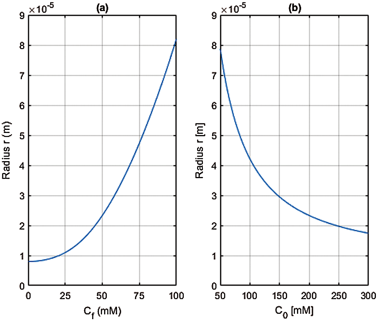
Figure 1: Steady state cell radius r computed from Eq. (63) with r0 = 8 × 10−6 m and K=1.25×10−2  N/m. (a) Variation of fixed charge concentration Cf with extracellular concentration C0 = 200 mM, (b) Variation of extracellular concentration C0 with fixed charge concentration Cf=50 mM

For active ion transport at steady (nonequilibrium) state (drdt=dC1dt=dC2dt=Jv= J1 = J2 = 0 with J1a≠0 and/or J2a≠0 and steady), the fluid pressure is given by ΔP = Δ Π + ΔPa (see (46)). The steady state cell radius for active ion transport is then found from (57)2 as

r=r024K(ΔΠ+ΔPa)+r02+(r024K)2(ΔΠ+ΔPa)2(64)

where Δ Π and ΔPa are evaluated using (54) and (55), respectively.

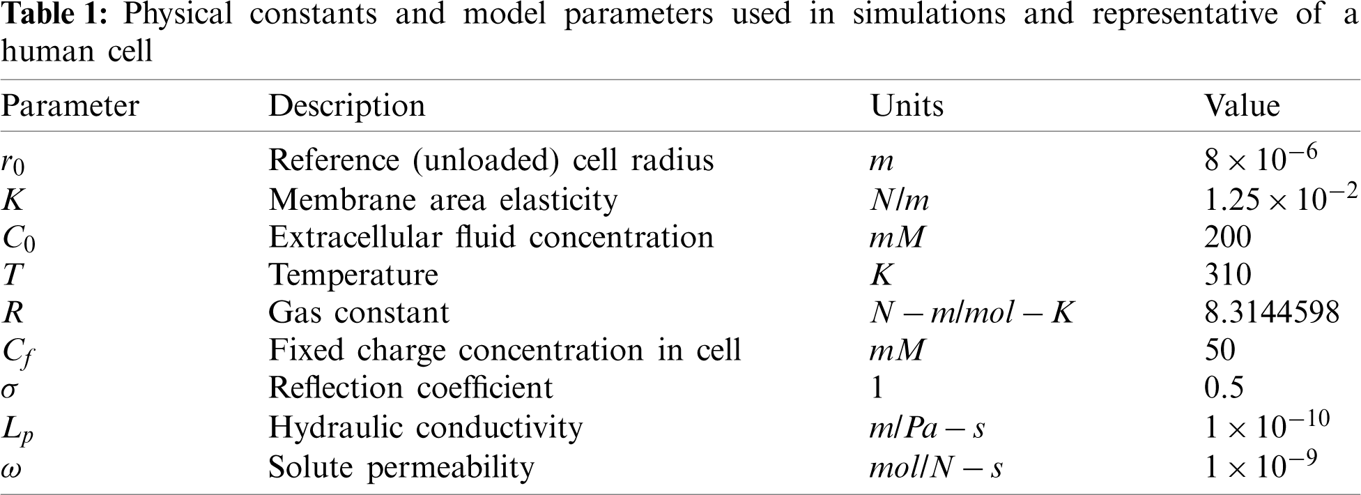
Fig. 2 examines the steady state cell radius based on (64) resulting from active transport of the cation only with β1=J1a/(RTω) and β2 = 0. All parameters employed are taken from Table 1. The steady state cell radius depicted in Fig. 2 demonstrates the steady state limit of the pump-leak mechanism in which active ion pumping reduces the osmotic pressure, causing the cell volume to contract as water passively transports out across the cell membrane. The effect of cation pumping on the steady state fluid and osmotic pressures are examined next.

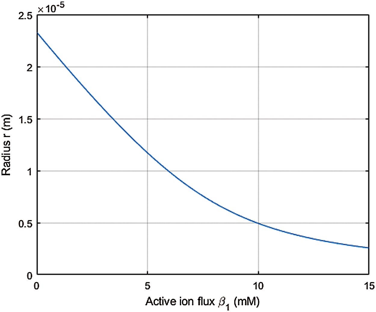
Figure 2: Steady state cell radius r (m) with active cation transport as measured by β1  (mM) and with β2=0. The cell properties are taken from Table 1. Increasing the cation pumping rate β 1 decreases the steady state cell radius

The steady state values of Δ Π and ΔPa are plotted in Fig. 3 against β 1 using (54) and (55), along with ΔP derived from ΔP = Δ Π + ΔPa. As active cation transport increases through β1, both osmotic and fluid pressure decrease significantly. The difference between them is ΔPa, which increases with β 1. Thus the fluid pressure reduction trails that of the osmotic pressure. It can be observed from Fig. 3 that at β 1≈ 7 mM, the fluid pressure difference becomes negative and the membrane state will transition from tension to compression. This is confirmed by Fig. 2 which indicates that the steady state equilibrium radius at β1 = 7 mM is r=8×10−6  m, which is the cell reference radius r0. Fig. 3 demonstrates quantitatively how increasing active ion transport reduces the osmotic and fluid pressures and thereby provides cell volume osmoregulation. The temporal solution of the model system (59) and (60) provides further insights into the PLM and is considered next.

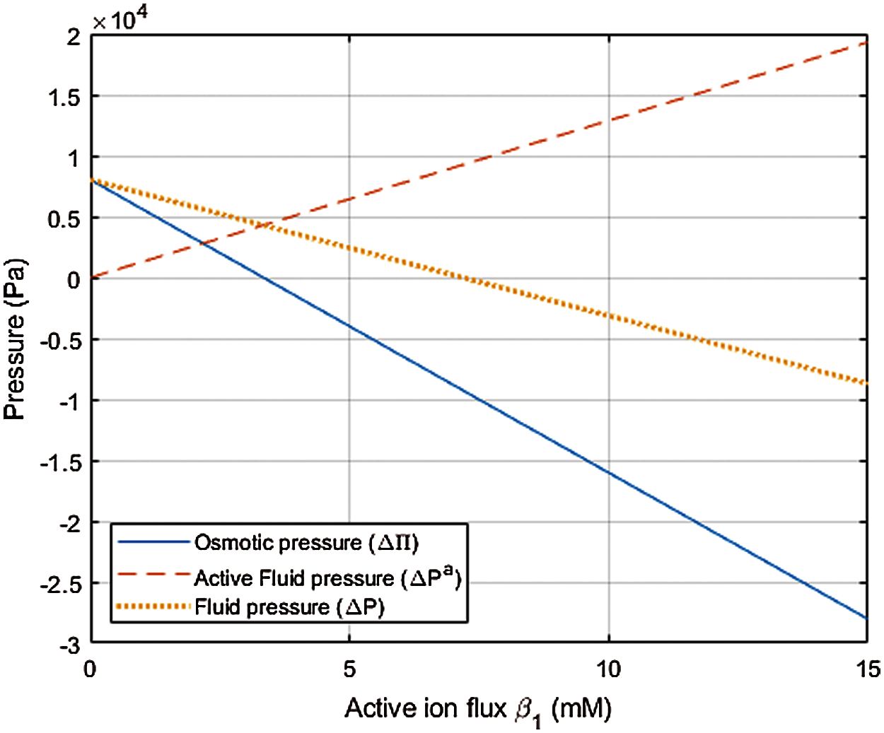
Figure 3: Plot of osmotic pressure ΔΠ, active fluid pressure ΔPa and fluid pressure ΔP vs. active cation flux β 1 (with no anion active flux β2=0). Cell properties are taken from Table 1

6  Temporal Response of the Pump-Leak Mechanism

6.1 Cell Response Simulations

Characterizing the details of ion channels and pumps is an active area of research that is beyond the scope of the present work. Nevertheless, a primitive example of an ion channel control model for homeostasis is provided in Section 6.3 to illustrate the ability of the proposed phenomenological equations to describe the pump-leak mechanism (PLM).

Two sets of numerical simulations are presented. In the first, the temporal response of the cell with only passive ion transport to a sequence of osmotic shocks is described in Section 6.2. Steady state results inferred from the temporal analysis are compared to the theoretical predictions given in Section 5 and provide a consistency check for the numerical implementation. In the second set of calculations, the PLM is simulated with active cation pumping. The initiation of active cation (Na+) pumping occurs when a tension-based cell membrane signal is received and subsequent changes in cell volume, fluid and osmotic pressure are reported in Section 6.3.

The physical constants and model parameter values given in Table 1 are used in all simulations, unless otherwise noted.

6.2 Passive Ionic Transport with Osmotic Shock

The cell was given arbitrary initial values of r(0)=8×10−6  m, C1(0)=210 mM and C2 = 190 mM, and allowed 1000 s to achieve near steady state. The cell is then subject to a hypotonic shock at t = 1000 s in which the extracellular ionic concentration C0 reduces from 200 to 120 mM. This is followed by a hypertonic shock at t = 2000 s in which C0 increases from 120 to 480 mM. This is described by

C0(t)=200[1−0.4H(t−1000)+1.8H(t−2000)](65)

where H is the Heaviside step function2. Solution of the three coupled ODEs (59) and (60), with β1 = β2 = 0 (no active ion pumping), was obtained using commercial software COMSOL Multiphysics 5.5. As seen in Fig. 4, the time interval between the initial (arbitrary) state and application of the two shocks was sufficient to allow the solution to closely approach three equilibrium states. As a validation of the temporal solution, the steady state radius and (Donnan) ionic concentrations and osmotic pressure was computed using (63), (36) and (37), respectively, at the three step levels of C0 in (65) and are given in Table 2. It may be confirmed from Fig. 4 that these values are the steady state asymptotes achieved in the temporal solution.

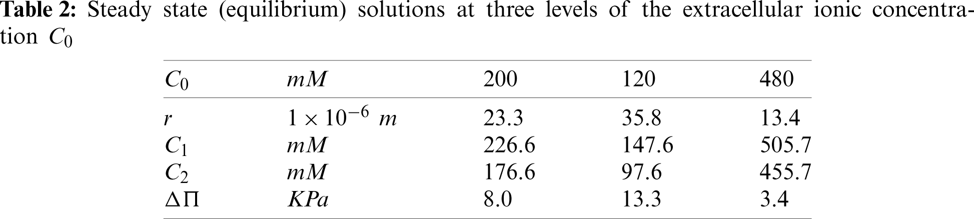
It may be observed in Fig. 4 that the cell radius achieves equilibrium at a slower rate than the ionic concentrations. This is expected because the rate of water transport across the membrane is controlled by the hydraulic conductivity Lp. When the hypotonic shock is applied at T = 1000 s, the volume flux Jv shown in Fig. 4d jumps to a negative value, indicating water inflow, but the slow tail of the passive inflow accounts for the slow response of the cell volume. Similarly, when the hypertonic shock is applied, the volume flux jumps to a positive value, indicating water outflow, with a time course dictated by the constant hydraulic conductivity. It may be noted from Fig. 4c that the osmotic pressure in the cell increases after the hypotonic shock and reduces after the hypertonic shock, as expected. Fig. 4b indicates that the cation and anion concentrations satisfy electroneutrality C1 − C2 = Cf = 50 mM at all times. It is remarked that the cell generates fluid pressure (not shown) by virtue of the elastic cortex—lipid membrane system and at steady state it is indeed in Donnan equilibrium.

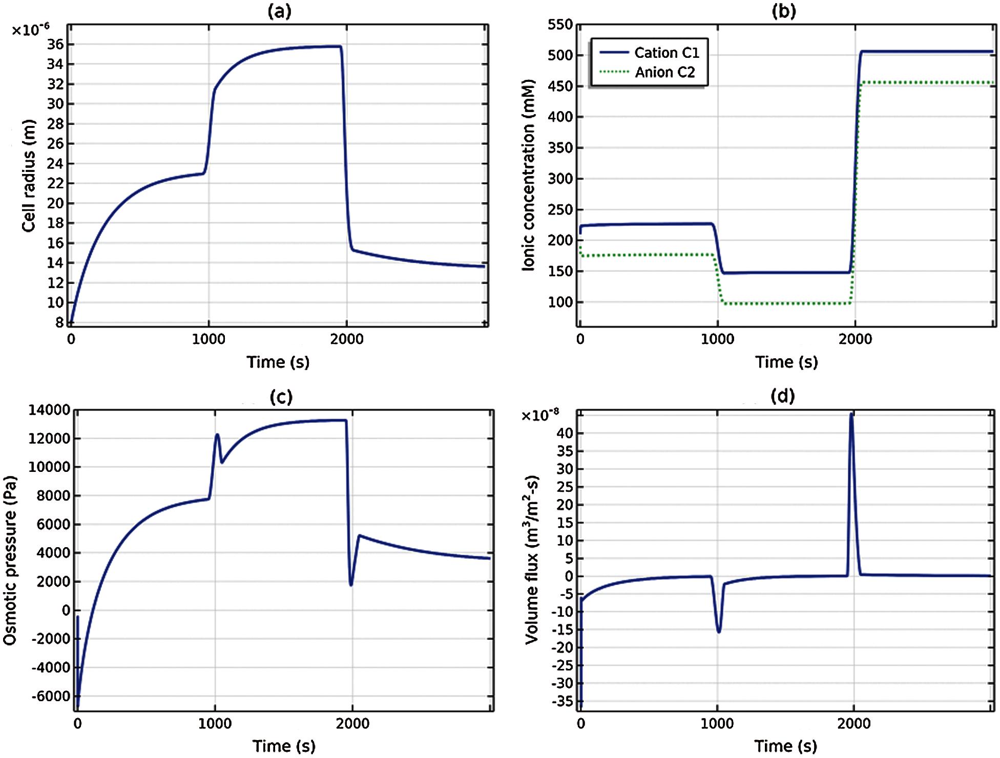
Figure 4: Transient response of the cell, with only passive ionic transport, to the osmotic shock loading given by (65): (a) Cell radius, (b) cation and anion concentrations, (c) osmotic pressure, (d) volume flux

6.3 Active Ionic Transport with Osmotic Shock

Using the same arbitrary initial values noted in the preceding subsection, 1000 s is allowed for the system to reach near steady state. The cell is then subject to a single hypotonic shock at t = 1000 s according to

C0(t)=200[1−0.6H(t−1000)](66)

Active cation (Na+) pumping is initiated when the membrane tension τ = τcrit. For this simulation, we assumed τcrit=5×τphysio where τphysio is the membrane tension when the cell is at equilibrium with C0 = 200 mM. Cation pumping is described by the value of β1 (see (50)), which was taken to be constant once activated. Then active transport by cation pumping is described by

β1(t)=β¯1H(τ(t)−τcrit)andβ2(t)=0(67)

with active flux magnitude β¯1=8.54 mM.

Fig. 5 compares two solutions. The solid (blue) curves correspond to passive transport only β1(t)=β2(t)=0) and the dotted (green) curves correspond to the active transport case defined by (67). It is remarked that the active flux magnitude β¯1 was selected to approximately return the cell radius to its previous steady state value—a parametric study on β1 is provided below. Fig. 5 indicates that cation pumping was initiated, according to (67), at approximately t = 1,250 s and that it has a pronounced effect on all solution variables. Most notably, the cell swells (measured by the radius r) under passive transport conditions following application of the shock. It then deswells under active transport conditions. The activation of cation pumping changes the cation molar flux from inflow to outflow Fig. 5b, and significantly depresses the osmotic pressure Fig. 5c. It may be confirmed that the steady state radius for the passive and active cases shown in Fig. 5 are predicted by (63) and (64), respectively.

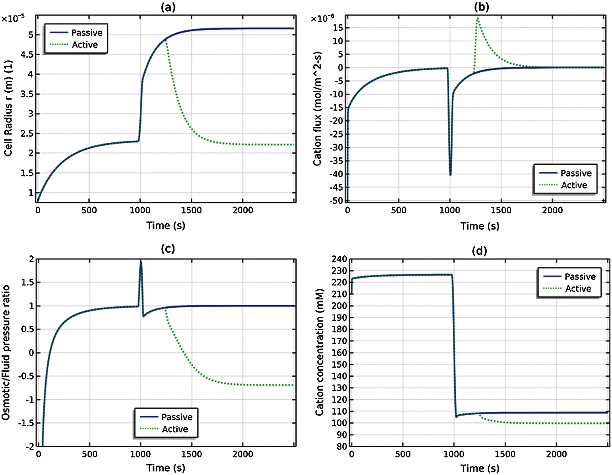
Figure 5: The cell is subjected to a hypotonic shock at t = 1000 s and two solutions are depicted. The solid (blue) curve shows the passive transport case and the dotted (green) curves show the active transport case: (a) cell radius r(t), (b) cation flux J1(t), (c) ratio of osmotic and fluid pressure ΔP(t)/ΔΠ(t), and (d) cation concentration C1(t)

Fig. 6a shows a side-by-side comparison of the osmotic and fluid pressures for the passive transport solution; Fig. 6b shows the same comparison for the active transport solution. It is seen from Fig. 6a that at steady (equilibrium) state (t = 1000 and t = 3000 s), the fluid and osmotic pressures coincide (as necessary, see (35)), whereas in Fig. 6b the osmotic and fluid pressures deviate significantly at steady (nonequilibrium) state (t = 3000 s) due to the active cation transport. The difference between the osmotic and fluid pressures is the active pressure component ΔPa = ΔP − ΔΠ given by (48). At steady state (t = 3000 s) and using (55), ΔPa=2RT(1−σ)βm≈11 kPa; from Fig. 6b we see that ΔP ≈ 6 kPa and Δπ≈ −5 kPa, which is in agreement. Observe that ΔPa is of the same order as ΔP and ΔΠ for ion pumping at β¯1=8.54 mM.

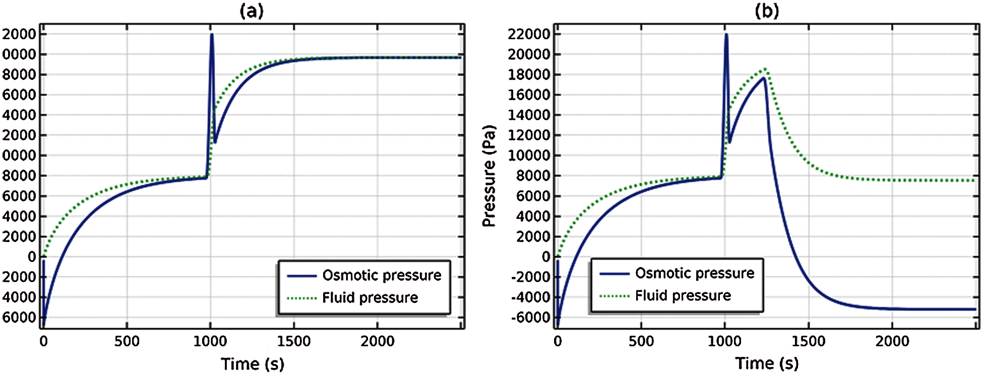
Figure 6: Comparison of osmotic and fluid pressures. (a) Passive transport solution, (b) Active cation transport solution

The results of a parametric study of the osmotic shock problem (67) is provided in Fig. 7. Figs. 7a and 7b show the cell radius and osmotic pressure for β1={3,6,9}; the radius and osmotic pressure decrease with increasing cation pump rate β1. Figs. 7c and 7d show the cell radius and osmotic pressure for the reflection coefficient σ={1,0.5,0} and β1 given by (67). When σ = 1, the membrane is semipermeable and the cation cannot transport passively across the membrane. At this limiting value of σ and at steady state, we have ΔPa=0 (see (55)) and the fluid and osmotic pressures will agree. When σ = 0.5 (the reference state used in Table 1), the membrane is leaky and the cation is transported passively and actively. When σ = 0, the membrane is nonselective and the cation is freely transported.

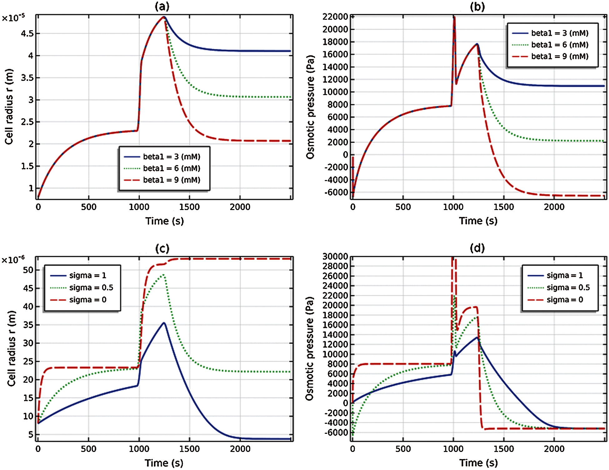
Figure 7: Parametric studies. (a) and (b) Active cation flux magnitude β1∈[3,6,9] mM, (c) and (d) reflection coefficient σ∈[1,0.5,0]

7  Discussion

The presented development of the phenomenological equations for passive and active transport for cell membranes follows standard lines for nonequilibrium thermodynamics. But an important step for electrolytes with impermeant charged macromolecules included the incorporation of fixed charge through the condition of electroneutrality. For passive transport of ionic solutions and at steady state, the theory recovers the Donnan equilibrium and predicts agreement of the osmotic and fluid pressure differences across the membrane such that ΔP = ΔΠ. When active ion transport processes are present, the theory predicts that an active fluid pressure component ΔPa arises as a direct result of the active fluxes. This term enters into the balance of fluid and osmotic pressure such that ΔP=ΔΠ+ΔPa. When the membrane is leaky, with σ < 1, numerical results indicate that ΔPa can have values that are of the same order as Δπ. The presented theory has included the fluid pressure in a rigorous manner through the phenomenological equations providing a general framework for assessing its role in the PLM.

The model evaluated the membrane potential Δψ by using the assumption that it is not changing rapidly with time. This led to the condition that the sum of the active and passive currents vanish Ip+Ia=0. The resulting expressions for Δψ (see (41)) generalize previous models such as that presented by Armstrong [2] to include the influence of the ionic reflection coefficient σk and ionic permeability ωk.

Following presentation of the general theory for an arbitrary number of ionic species, the theory was adapted to model the pump-leak mechanism (PLM) in a eukaryotic cell model. The cell was modeled as a spherical elastic shell with area elasticity but no attempt was made to model the dependence of the modulus on the cell volume or other possible structural characteristics. However, the cell cortex—lipid membrane system so modeled was able to develop tension and support fluid pressure—allowing both fluid and osmotic pressures to be modeled and studied for both passive and active transport. The intracellular and extracellular media were taken to be simple binary electrolytes containing Na+ and Cl− ions. Trapped (nonpermeant) charged macromolecules were included in the intracellular medium but no attempt was made to model the “excluded volume” effects associated with the molecular volumes (this is essentially treated by specification of an effective charge concentration Cf). Temporal changes in concentrations took account of membrane transport processes and the dynamically evolving cell area and volume. Active ion transport results were reported using an Na+ pump to stabilize cell volume against osmotic forces that would otherwise drive water into the cell.

The PLM mechanism is clearly demonstrated in Fig. 8. The problem solved is that described in Section 6.3; the cell is subjected to a hypotonic shock at time t = 1000 s, at which time it begins to swell as indicated by the increasing cell radius and the jump in water inflow (negative values of Jv). Initiation of Na+ pumping occurs when the membrane tension reaches a critical value, at time t ≈ 1,250 s. The cell volume now starts to decrease and approach a steady state. The direct correlation of Na+ active flux with water outflow (positive values of Jv) is apparent in the figure and suggests capture of the PLM.

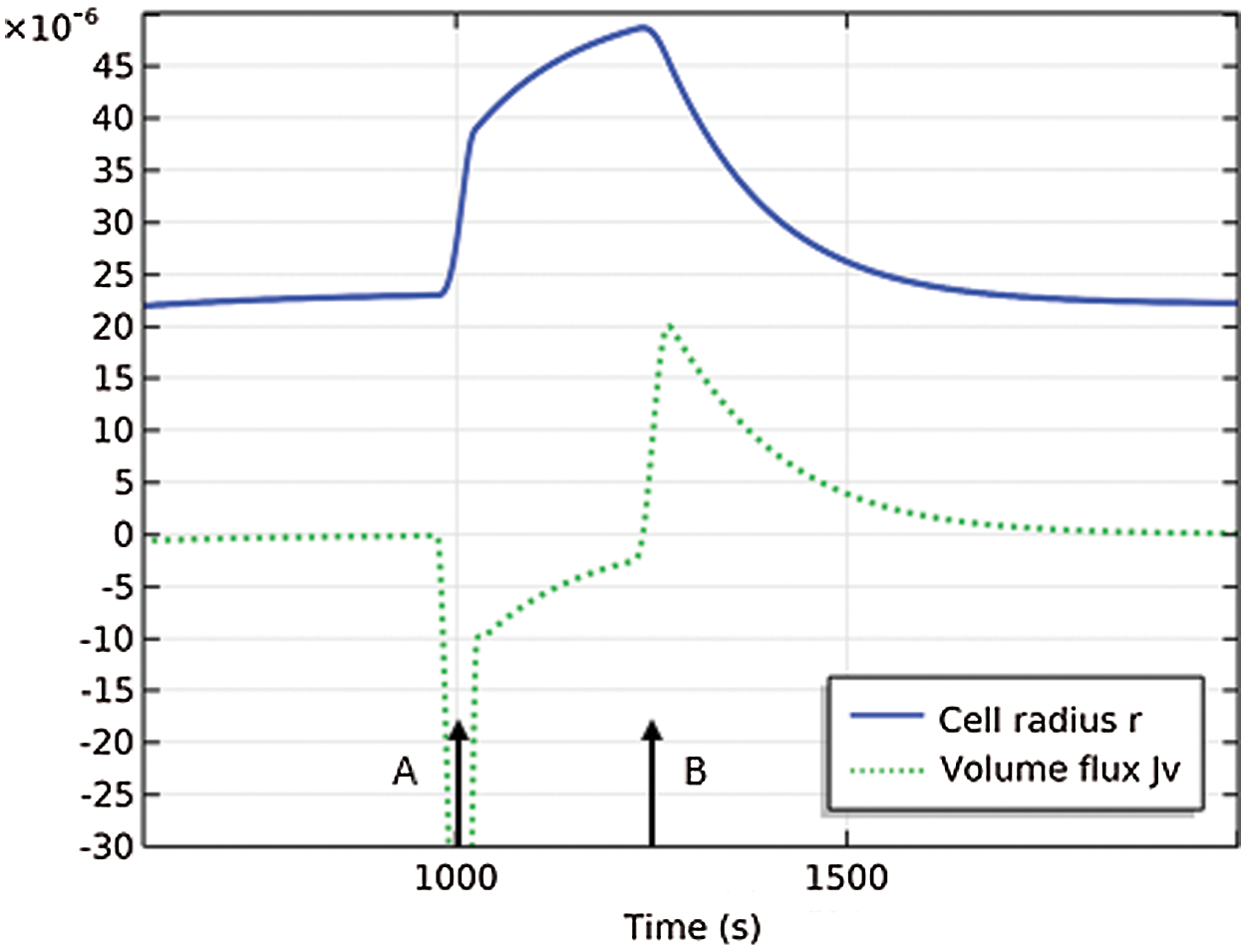
Figure 8: Cell undergoes hypotonic shock at time A and initiates active cation pumping at time B. The cell radius is r(m) and the volume flux is Jv (mol/m2 − s) and has been scaled by 120. At time A, the cell begins to swell by water inflow. At time B, the cell begins to deswell by water outflow

Previous models of the PLM, presented in the field of mathematical physiology have been successful in demonstrating the key aspects of the mechanism [2,3,5,19]. However these models cannot exhibit a stable Donnan equilibrium, in contrast to the current study. Cells cannot be at a stable Donnan equilibrium unless they can develop and sustain a transmembrane fluid pressure. For example, in prior models, if ions are not actively pumped, the cell volume will increase without limit and no steady state will be found. The current model develops fluid pressure and arrives at steady state according to the hydraulic conductivity (see, for example, Fig. 5a). It has been claimed that cells cannot be at a stable Donnan equilibrium, but this is true only if they cannot support internal fluid pressure [20]. The current model shows clearly that in the case of passive ion transport, Donnan equilibrium can be achieved using realistic values of the cell membrane elasticity.

In practice, the primary contributors to intracellular and extracellular tonicity are Na+, K+ and Cl− , all of which are permeable solutes. The Na+ pump (Na+ − K+ ATPase) actively drives Na+ out and K+ in [5,21]. Ion channels and ion pumps drive the physiological system, aquaporins (water channels) likewise modulate the hydraulic conductivity of the cell membrane. These essential features underlying the PLM can be modeled within the presented framework, based on experimental evidence, and would provide a more complete representation of the PLM.

Since we have no knowledge of how Ck varies across the membrane, a good approximation is:

C¯k=12(Ck+Ck0)with C¯k=12(Ck+Ck0). Forexample, if Ck=300 and Ck0=100, the approximation error is 9%.

The Heaviside functions H(t − tshock) were smoothed over a transition zone of 100 s in order to be more physically realistic.

Funding Statement: The author received no specific funding for this study.

Conflicts of Interest: The author declares that they have no conflicts of interest to report regarding the present study.

This work is licensed under a Creative Commons Attribution 4.0 International License, which permits unrestricted use, distribution, and reproduction in any medium, provided the original work is properly cited.