Matrix-Free Higher-Order Finite Element Method for Parallel Simulation of Compressible and Nearly-Incompressible Linear Elasticity on Unstructured Meshes

Arash Mehraban; Henry Tufo; Stein Sture; Richard Regueiro

doi:10.32604/cmes.2021.017476

1Department of Computer Science, University of Colorado Boulder, Boulder, CO, USA
2Department of Civil, Environmental, and Architectural Engineering, University of Colorado Boulder, Boulder, CO, USA
*Corresponding Author: Richard Regueiro. Email: richard.regueiro@colorado.edu
Received: 13 May 2021; Accepted: 02 July 2021

Abstract: Higher-order displacement-based finite element methods are useful for simulating bending problems and potentially addressing mesh-locking associated with nearly-incompressible elasticity, yet are computationally expensive. To address the computational expense, the paper presents a matrix-free, displacement-based, higher-order, hexahedral finite element implementation of compressible and nearly-compressible (ν→0.5) linear isotropic elasticity at small strain with p-multigrid preconditioning. The cost, solve time, and scalability of the implementation with respect to strain energy error are investigated for polynomial order p = 1, 2, 3, 4 for compressible elasticity, and p = 2, 3, 4 for nearly-incompressible elasticity, on different number of CPU cores for a tube bending problem. In the context of this matrix-free implementation, higher-order polynomials (p = 3, 4) generally are faster in achieving better accuracy in the solution than lower-order polynomials (p = 1, 2). However, for a beam bending simulation with stress concentration (singularity), it is demonstrated that higher-order finite elements do not improve the spatial order of convergence, even though accuracy is improved.

Keywords: Matrix-free; higher-order; finite element; parallel; linear elasticity; multigrid solvers; unstructured meshes

Modeling bending deformation and associated stress of compressible and nearly-incompressible linear isotropic elastic materials via the standard linear interpolation displacement-based Finite Element Method (FEM) may lead to inaccurate stress calculations (depending on element size h) as well as potential mesh-locking [1,2]. With respect to accuracy, either h-or p-refinement are adopted, but oftentimes not the two together because of the associated high computational cost. With respect to mesh-locking, several FEM approaches involving mixed formulations have been proposed to overcome volumetric strain locking of linear finite elements [3–6]. Most such mixed methods for linear elasticity at small strain solve for two fields (displacement and pressure), which are discretized separately via an additive split of the deviatoric and volumetric parts of the small strain tensor [7,8]. As an alternative to, and oftentimes in conjunction with, mixed formulations, higher-order finite elements have been adopted to attempt to overcome mesh locking [9]. However, assembling a global Jacobian matrix based on higher-order finite element interpolation functions leads to expensive solve times as a result of higher memory requirements [10]. Matrix-free formulations [11,12] provide the benefits of higher-order finite element methods but with more efficient memory usage. Concurrently, using tensor-product-basis evaluation further improves the performance of higher-order methods by supplying favorable storage and work estimates of O(pd) and O(pd+ 1) per p-order element, respectively, for discretizations in Rd [11], where d denotes spatial dimension. Furthermore, tensor-product-based operator evaluations can be cast as matrix-matrix products. Iterative solvers, such as Krylov subspace methods, only require the result of matrix-vector products rather than an assembled matrix, which allows these methods to take advantage of the computational efficiencies offered by matrix-free formulations. Therefore, storage of large, sparse matrices is avoided with iterative solvers.

Krylov subspace methods require preconditioning [13] to efficiently and stably solve large-scale elliptic problems such as 3D linear isotropic elasticity within the static balance of linear momentum equations. Geometric multigrid is a robust preconditioning scheme that is an appealing choice for structured meshes, and has been considered in numerous studies using finite difference and finite element methods with tensor-product-bases implemented on CPUs and GPUs [14–16]. p-multigrid, developed by Rønquist et al. [17], is a version of geometric multigrid based on coarsening by decreasing the basis order in higher-order or spectral finite elements rather than coarsening by aggregating elements. As a result, p-multigrid is a natural approach for problems on unstructured meshes, whereby spatial convergence only weakly depends on polynomial order p, if properly implemented. Computational cost of the discretization scheme may be affected by polynomial order p and element size h, among other factors [18,19], such as adaptive r-refinement of the mesh [20].

In terms of engineering applications, compressible linear isotropic elasticity (e.g., ν = 0.3) is appropriate for modeling metals in their elastic regime, such as in serviceability studies to analyze the stress intensity factor at a crack tip to determine if the crack will propagate and thus estimate the life cycle of a metallic component. Nearly-incompressible linear isotropic elasticity (ν→0.5) is appropriate for modeling small deformations (small strains and small rotations) of rubber-like materials such as solid rock propellant binders [21]. When metals or rubber-like materials are loaded beyond their small strain linear elastic limit, then large deformation hyperelasticity or hyper-elasto-plasticity constitutive models are needed, which are beyond the scope of this paper.

In this work, we apply a previously-developed matrix-free, higher-order, FEM for solving three-dimensional (3D) linear isotropic elasticity with p-multigrid preconditioning [22,23] to (i) a tube geometry subjected to method of manufactured solutions (MMS), (ii) a tube bending problem for compressible (ν = 0.3) and nearly-incompressible (ν = 0.499999) elasticity and polynomial order p = 1, 2, 3, 4, and (iii) a beam bending problem under body force loading for which the beam is clamped on both ends. Simulations (ii) and (iii)—but simulation (iii) in particular—cause a stress concentration (singularity) in the clamped regions, where the higher-order FEM may not converge optimally as expected [22]. Therefore, we investigate order of convergence of the matrix-free higher-order FEM for compressible elasticity when there is a stress concentration. We aim to answer the following questions: (1) With the matrix-free parallel implementation, what combination of mesh-refinement h and polynomial order p leads to a certain strain energy error that requires the least computational cost for compressible and nearly-incompressible elasticity using the standard displacement-based FEM? (2) What combination of mesh-refinement h and polynomial order p achieves a certain strain energy error for least amount of simulation time? (3) Does the higher-order, displacement-based FEM remain competitive as Poisson’s ratio approaches the nearly-incompressible limit (ν→0.5)? (4) Does the higher-order FEM converge as expected when there is a stress concentration present? The parallel computational toolkit PETSc [24] is employed for the linear solver as well as Algebraic MultiGrid (AMG) preconditioner for the coarse-grid solve, while libCEED [25] is used to perform efficient tensor-product-basis evaluation.

The rest of the paper is organized as follows. In Section 2, the constitutive model for compressible 3D linear isotropic elasticity and the variational form of static balance of linear momentum are presented. In Section 3, a preconditioning scheme used to accelerate convergence is briefly discussed. In Section 4, numerical results are presented, and in Section 5, observations and conclusions are provided.

For linear isotropic elastic materials, we consider the stored strain energy function as,

Therefore, its stress-strain relationship is given by its derivative with respect to strain as,

where ϵσ and are stress and strain tensors, respectively; and λ and μ are the Lamé parameters. The small strain tensor is,

The strong form of the static balance of linear momentum is given by the following,

where the functions u¯ and t¯ are prescribed boundary displacement and traction, respectively, g is the body force per unit mass (such as the gravitational acceleration vector), and ρ is the mass density. Introducing weighting function w for the displacement field, the corresponding variational equation for (4) is written as,

Discretization of the variational Eq. (5) can be written to facilitate matrix-free evaluation [10]. The residual in discrete form can be expressed as,

∑eεeT[ (Ne)T⋅W⋅Λ(f0(ue,∇ue))+∑i=1dim(Bie)T⋅W⋅Λ(f1(ue,∇ue)) ]=0 (6)

where Ne and Bie are evaluations of the finite element shape functions and their derivatives at the quadrature points in x, y, and z directions, εe is the element e restriction operator that separates Degrees of Freedom (DoF) based on the elements to which they belong, and represents pointwise function evaluation. f0 and f1 are determined from the constitutive model and its tangent, where ue=Ne(εed) and ∇ue=∑I=1dim[Bie(εed)], and d is the total nodal displacement vector. The basis operators are represented as Kronecker products,

where N^ and B^ evaluations of the finite element shape functions and their derivatives at the quadrature points in 1D. Comparing the variational equation in (5) to its discrete form in (6) yields f0=g and f1=σ, assuming t¯=0.

Similar to a residual evaluation, the action of the Jacobian can be computed using the notation proposed by [10,26], as,

In the small strain case, for Eq. (2), f0 is not a function of u or ∇u. Therefore, its derivative with respect to u or ∇u is zero, (i.e., f0,0=0 and f0,1=0). On the other hand, f1 is a function of ∇u, but it is not a function of u. Therefore, f1,0=0 and f1,1=∂σ/∂ϵ; due to linearity, ∂σ/∂ϵ=λI⊗I+2μI, or equivalently, f1,1(∇δu)=(∂σ/∂ϵ):∇δu=λtr⁡[ϵ(δu)]+2μϵ(δu), which is equivalent to (2) applied to an increment δu within a nonlinear iterative solver. While these minor simplifications are possible for linear problems in the present work, our implementation solves the problem as though it were nonlinear, and we will continue using the corresponding terminology.

Using the formulation in Eq. (8), we can compute the action of global Jacobian matrix on with arbitrary user defined polynomial order p. An iterative linear equation solver is required with matrix-free operators, which necessitates preconditioning, especially at higher-order. With unstructured meshes, a natural hierarchy of grids does not exist, so h-multigrid can be difficult to implement. Algebraic MultiGrid (AMG) is suitable for low order meshes for which the Jacobian matrix can be assembled. However, assembly of this matrix is prohibitively expensive for higher-order element meshes [27]. Therefore, we use geometric multigrid with p coarsening while adopting AMG as the coarse grid solver. A Chebyshev polynomial smoother based upon the operator diagonal [28] is called in the multigrid cycle.

In p-multigrid, grid transfer operations increase or decrease the polynomial order of the element basis functions, and these operations can be implemented in a matrix-free fashion via f0,0 of (8) with suitable basis evaluators N. The coarse-to-fine (ctof) basis operation, Nctof, interpolates the DoFs on the nodes of a coarse grid element to the nodes of a fine grid element (N27×8 for Q1 prolongation to Q2, for example, where Q1 denotes p=1 and Q2,p=2). The corresponding coarse and fine grid element restriction operators, εe,c and εe,f, are used in the grid transfer operators. The operator P=∑eεe,fTNctofεe,c correctly computes the interior degrees of freedom but over-counts nodes on the element facets. We can count the multiplicity of each node on the fine grid by applying the transpose fine grid restriction to the unit vector, ω=∑eεe,fT1. Thus, the p-multigrid prolongation operator is given by,

Using the 3D linear isotropic elasticity model and matrix-free, higher-order FEM presented in Sections 2 and 3, we present numerical results based on (i) method of manufactured solutions (MMS) applied to a tube geometry, (ii) a tube bending simulation for compressible and nearly-incompressible elasticity on unstructured meshes, and (iii) a beam bending simulation with stress concentration on structured meshes. Polynomial orders p = 1, 2, 3, 4 are applied for a range of meshes in the compressible case, and polynomial orders p = 2, 3, 4 are applied for the same range of meshes in the nearly-incompressible case. For the compressible case, Poisson’s ratio ν = 0.3 and Young’s modulus E = 69 × 109 Pa, that correspond to aluminum. For the nearly-incompressible case, ν = 0.499999 and E = 0.1 × 109 Pa, that correspond to rubber-like materials in the small elastic strain regime.

The parallel platform used to run all FE simulations with higher-order polynomial element meshes is an Intel Xeon E5-2680 v3 @2.50 GHz (2 CPUs/node, 24 cores/node) and 113 GB RAM per compute node [29]. The PETSc toolkit v3.14 is called for mesh management, domain decomposition, parallel assembly operations, and communication over all MPI processes. The matrix-free Jacobian operator is implemented using libCEED v0.8 and PETSc for Eq. (8). Preconditioning with p-multigrid and AMG is enabled through PETSc’s multigrid interface with grid-transfer and operator application at each level implemented in libCEED. Vectorized tensor-product operations for 8-element batches in the matrix-free operator evaluation on AVX-2 extensions of ×86 instruction sets for each local processor are conducted in libCEED. For simulations conducted with MMS and tube bending, an unstructured mesh consisting of 400 Hex8 elements (trilinear) is generated in the Trelis [30] software. The mesh is then refined 5 times to generate 3,200, 10,800, 25,600, 50,000, and 86,400 element meshes, respectively.

4.1 Achieving L2 Strain Energy Error via h- and p-Refinement in Tube Meshes Subjected to MMS

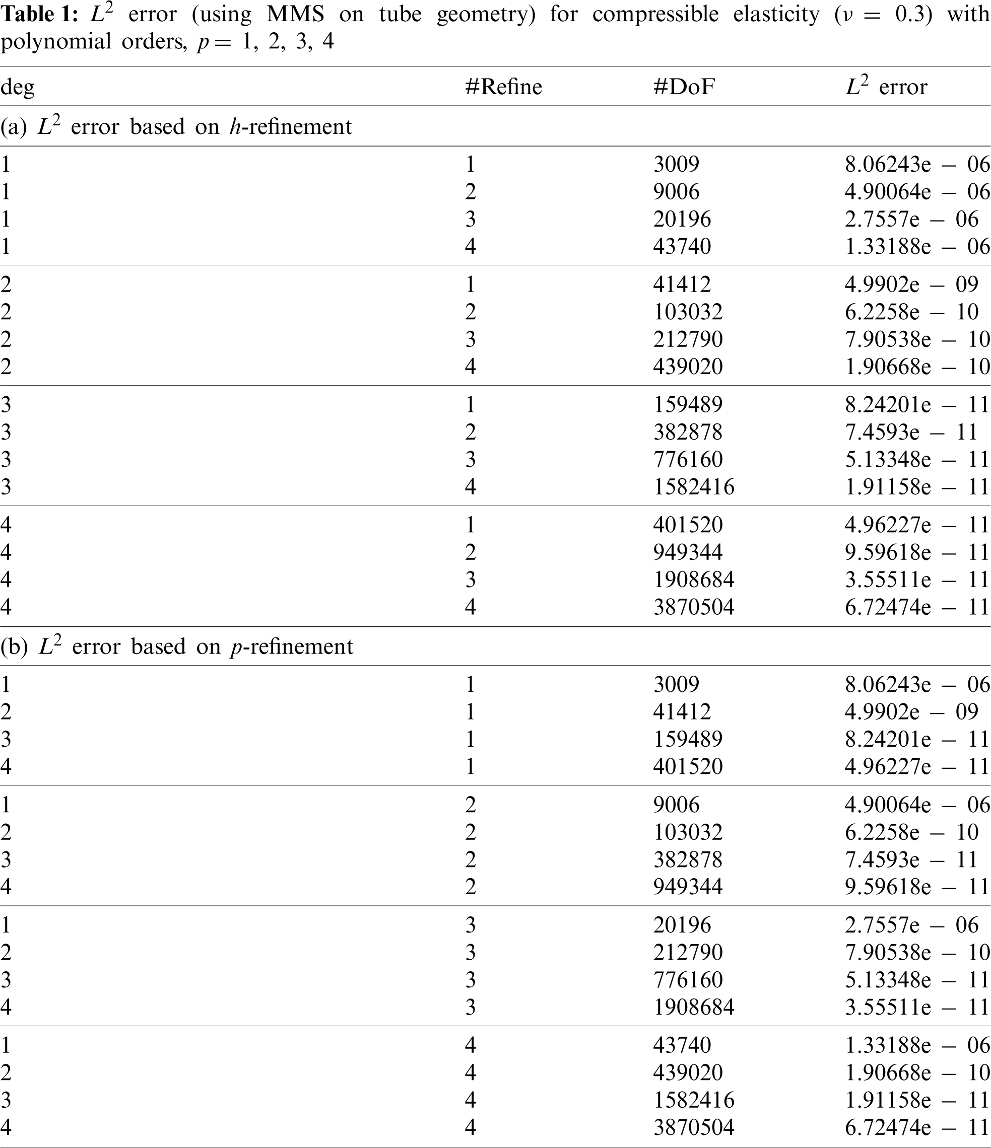
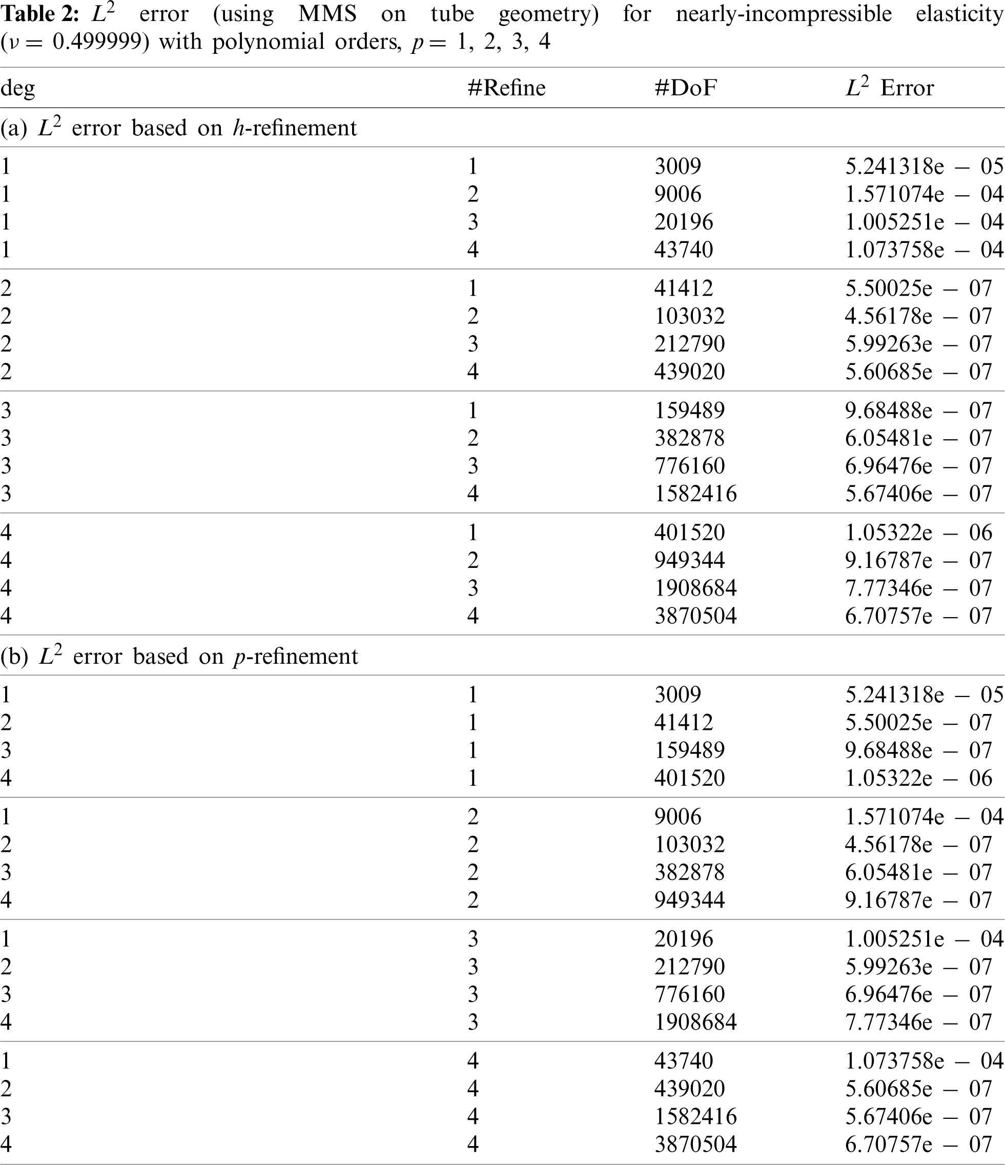
Considering the tube geometry in Fig. 1 with method of manufactured solutions (MMS)-generated displacement boundary conditions, the first four tube unstructured mesh refinements with 3,200, 10,800, 25,600, and 50,000 elements are used in the FE simulations for the compressible and nearly-incompressible cases. For the MMS, we produce a contrived, but smooth, right hand side ρ based on = [u1, u2, u3]T with u1 = e2x sin(3y) cos(4z)/108, u2 = e3x sin(4y) cos(2z)/108, and u3 = e4x sin(2y) cos(3z)/108. Every problem is run once to determine the L2 global strain energy Φh error from the MMS. Tables 1a and 1b summarize the size of each problem in terms of degrees of freedom (“#DoF”) based on h-and p-refinement and the corresponding L2 strain energy error based on MMS for the compressible case. Tables 2a and 2b summarize the size of each problem in terms of DoF based on h-and p-refinement and the corresponding L2 strain energy error based on MMS for the nearly-incompressible case. Considering the smoothness of the MMS, and relatively high number of DoF for even the coarsest mesh (3009 elements), the strain energy error is already quite small prior to refinement. Although, for p-refinement, we see for the compressible case some convergence, while for the nearly-incompressible case, the error is small and stays small (but not as small as the compressible case, 10−10 vs. 10−7) indicating stability for smooth deformations via MMS.

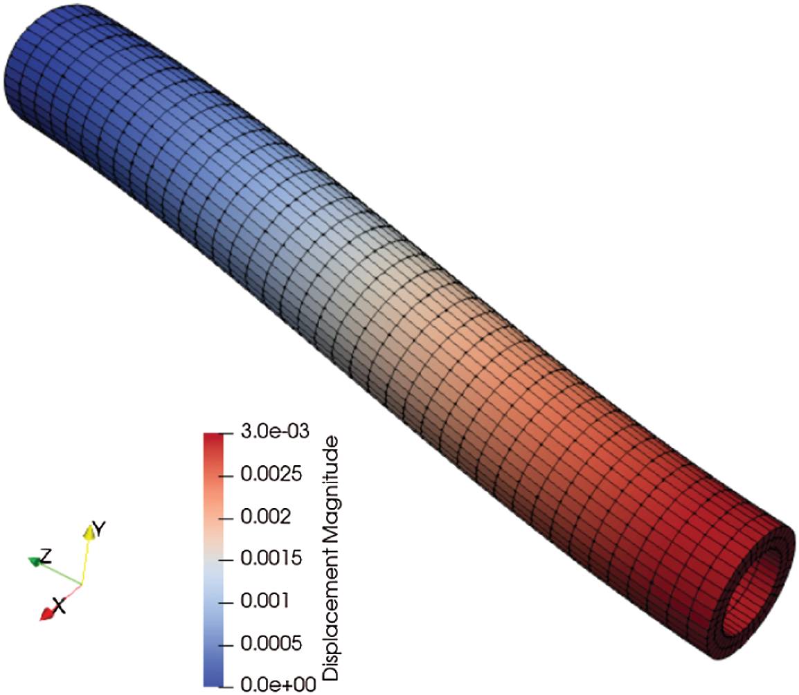
Figure 1: Deformed hexahedral mesh for the cylindrical tube bending problem. The length of the tube is 100 mm, with circular cross-section with inner diameter 15 mm and outer diameter 20 mm. The left wall is fixed in x, y, and z displacements, while the right wall is displaced in the negative y direction by 3 mm

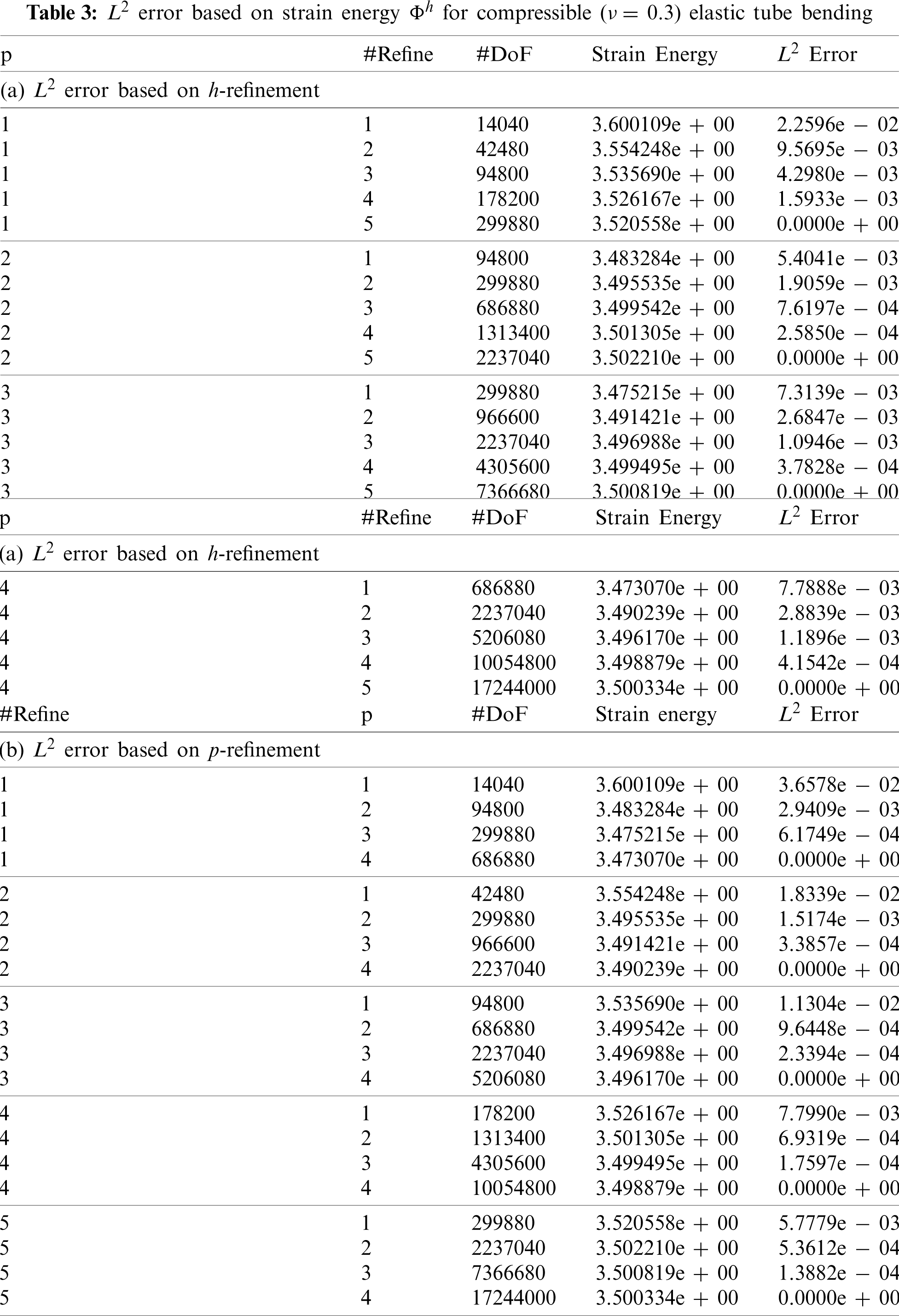
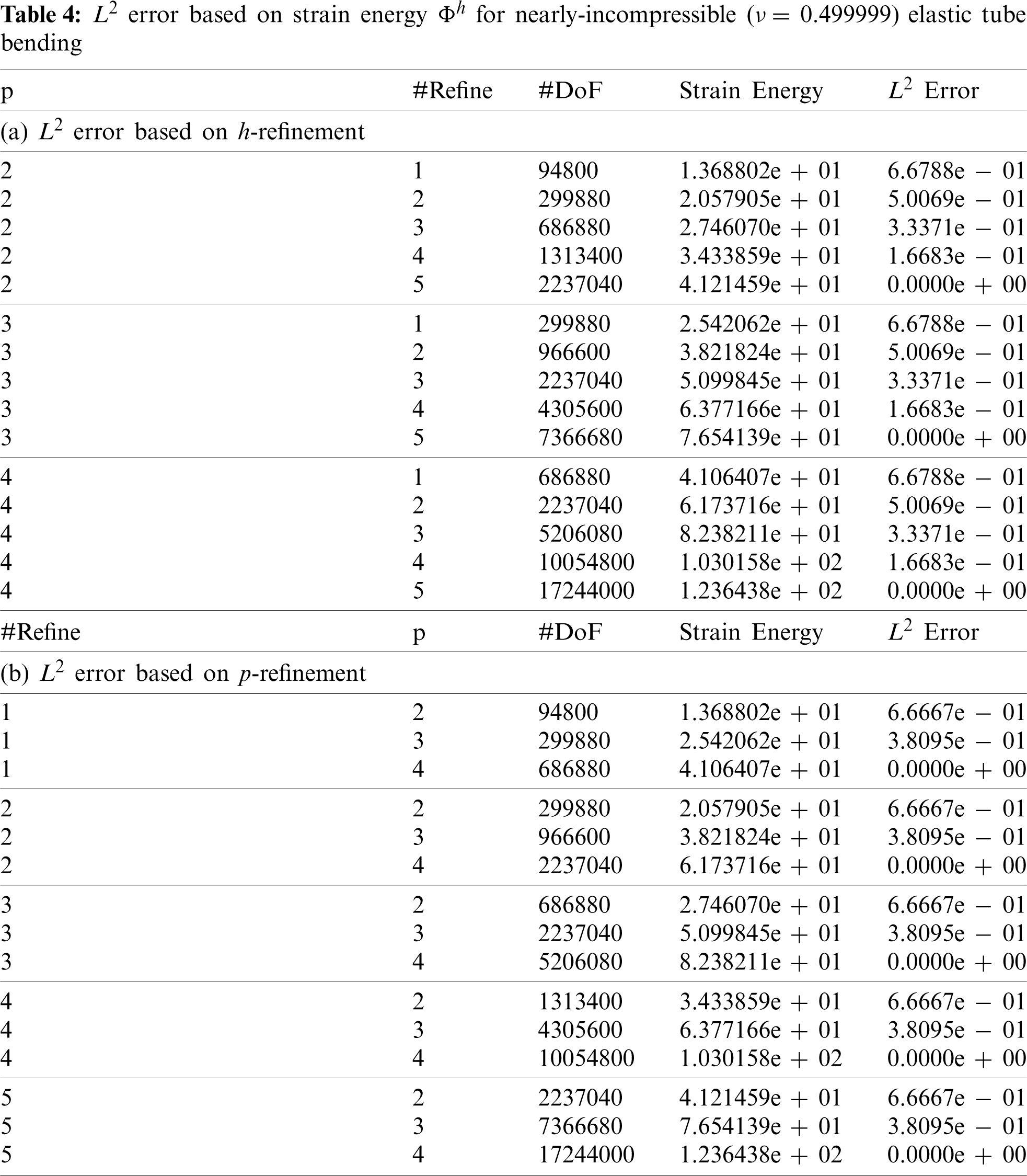
Tube meshes subjected to bending are simulated to study cost and spatial convergence of the matrix-free, higher-order FEM for h-refinement and p-refinement based on strain energy Φh for compressible and nearly-incompressible elasticity. The length of the tube is 100 mm, with circular cross-section of inner diameter 15 mm and outer diameter 20 mm. A coarse mesh representation of the tube is shown in Fig. 1. The left side of the tube is clamped by placing a zero displacement boundary condition on the surface, while a second displacement boundary condition is imposed on the right surface of the tube to bend it 3 mm in the negative y direction. Fig. 1 shows the deformed mesh after bending. All tube meshes are simulated for compressible and nearly-incompressible elasticity. Tables 3 and 4 summarize the problem sizes in terms of degrees of freedom (“#DoF”) for each refinement in conjunction with different polynomial orders p for compressible and nearly-incompressible elasticity, respectively. The size of problem (“#DoF”) increases when a finer mesh h or a higher-order polynomial p is used. As the FE mesh is refined in h, the norm of the strain energy computed from the FE solution converges to the exact norm of strain energy [31]. Therefore, we use the discrete elastic strain energy Φh to compute relative error in the FE simulations with respect to smaller size problems. Achieving a certain strain energy error in the FE solution is problem-dependent. For example, problems with smooth and non-smooth solutions behave differently with mesh refinement h when used with different polynomial orders p [18]. Therefore, with mesh refinement through decreasing h, we treat the strain energy from the finest mesh as the “exact” solution in the computation of relative L2 error for each polynomial order p to determine the effect of h-refinement in achieving a certain error. However, with p-refinement, we treat the strain energy from the highest polynomial order (p = 4) to compute the relative L2 strain energy error for each p-refinement. Tables 3a and 3b summarize the relative L2 error based on mesh refinement h and using higher-order polynomials p for the compressible tube bending FE simulations, respectively. In addition, depending on the problem, each simulation is run with 1, 6, 12, 24, 48, 96, 192, 384, and 768 CPU cores for the compressible case. Each simulation is run 3 times to reduce noise in the performance timing for a total of 297 simulations for the compressible case.

To address the first question raised in the Introduction with regard to minimal computational cost for a certain strain energy error in the FE solution for compressible elasticity, we compute the minimum amount of CPU work to reach a certain error based on mesh refinements and higher-order polynomials. To do this, for each polynomial order p we accumulate the time spent to reach the error. Then we determine the minimum time in the list and multiply it by the number of processors np that are executed for the minimum time. We generate Pareto optimal diagrams to present the results of the study for compressible and nearly-incompressible elasticity separately, where a point on the diagram is called Pareto optimal if strain energy error cannot be decreased (moving down the ordinate (y axis)) without increasing time (or cost) by moving to the right on the abscissa. The set of Pareto optimal configurations is known as the Pareto front.

Figs. 2a and 2b present the L2 strain energy error based on mesh refinement vs. cost, and the L2 error based on higher-order polynomials vs. cost, for compressible elasticity. Figs. 2a and 2b show that the minimal cost to achieve a certain error occurs in the lower left region of the diagram, indicating that higher order p is the most cost-effective for the compressible case. Each horizontal series of the same color represents a strong scaling study at fixed mesh refinement h and polynomial order p, but with changing number of processors np, with perfect strong scaling occurring when all color dots are collocated. The more expensive simulations tend to exhibit better strong scaling because they have more work over which to amortize the inherent communication costs, while smaller models (fewer DoFs) are more cost-efficient to run on a single core. The low order p = 1 cases are increasingly far from the Pareto front. In addition, solely calling larger number of CPU cores is less cost-efficient, although are faster with respect to solve time up to the point where the parallel overhead communication begin to dominate.

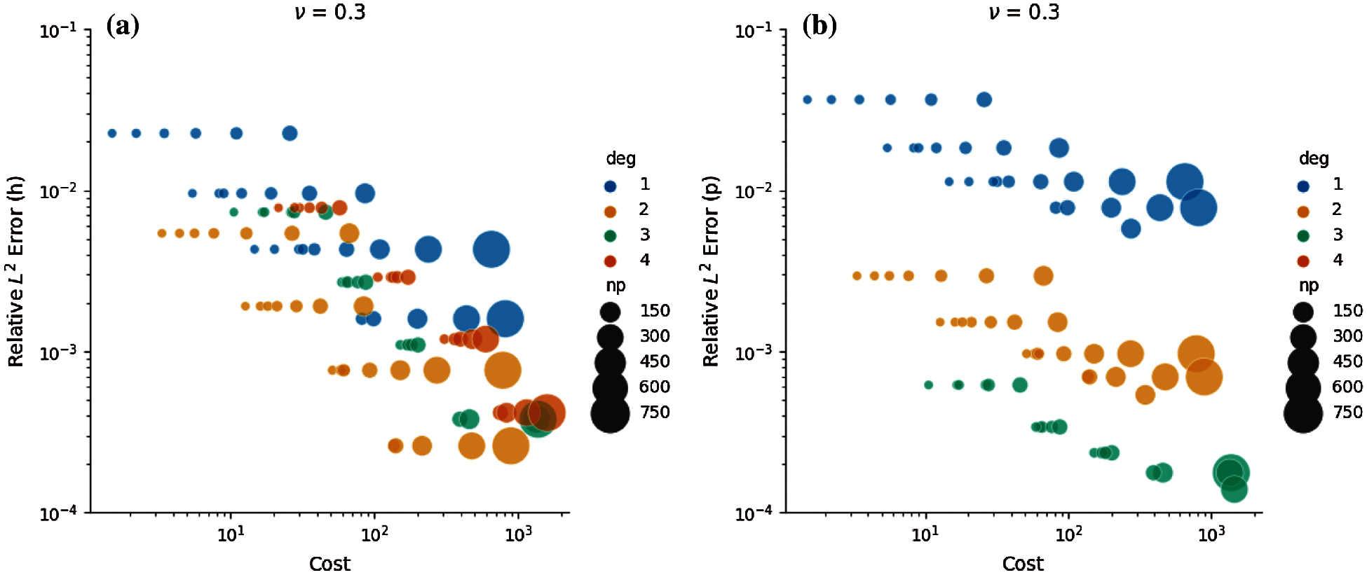
Figure 2: Error vs. cost for compressible elastic tube bending. The Pareto optimal configurations occur in the lower left region of the plot indicating a higher-order polynomial p is more cost-efficient for a certain error. (a) Error based on h-refinement vs. cost. (b) Error based on p-refinement vs. cost

To answer the second question raised in the Introduction regarding the least amount of time to achieve a certain strain energy error given enough computational resources, we provide a second set of Pareto optimal diagrams in Figs. 3a and 3b for the compressible elasticity tube bending problem. The Pareto optimal configurations are toward the lower left region of the plot, whereby upon p-refinement, p = 3 exhibits faster solve times for certain error, while upon h-refinement, p = 2 delivers the fastest solve times for certain error, a result that was unexpected and requires further investigation. Each horizontal series of the same color represents strong scaling of a given mesh refinement h and polynomial order p. Larger number of CPU cores when enough work is amortized tend to reach a certain error in the solution faster with higher order polynomials. Similar to Pareto optimal for the cost, strong scaling occurs when the same color larger dots overlay smaller dots.

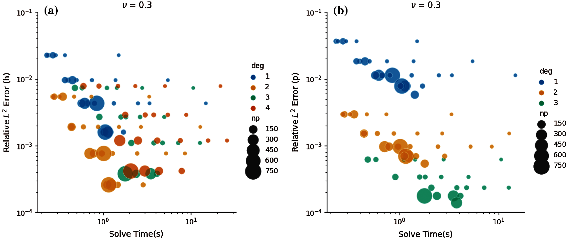
Figure 3: Error vs. time for compressible elastic tube bending. The Pareto optimal configurations occur toward the lower left region of the plot. (a) Error based on h-refinement vs. time. (b) Error based on p-refinement vs. time

We notice that depending on the error, increasing the polynomial order p while fixing mesh size (h constant) may provide the fastest time to solution. For example, for strain energy error between 10−3 and 10−4, polynomial order p = 3 may be faster than lower order polynomials, but for error greater than 10−3, polynomial order p = 2 may be faster. This could be due to the number of DoFs for different polynomial orders when run with the same size mesh. In addition, we expected that higher order polynomials p = 3, 4 would be more cost-efficient than lower order polynomials. However, we observed that polynomial order p = 2 is more cost-efficient than higher order polynomials p = 3, 4 for this compressible tube bending problem.

For nearly-incompressible elasticity, we use the same meshes h and polynomial order p. The problem sizes in terms of DoFs and L2 strain energy error based on mesh refinement and polynomial orders are represented in Tables 4a and 4b. However, we instead use 24, 48, 96, 192, 384, 768, and 1536 CPU cores since nearly-incompressible elasticity is more computationally intensive for matrix-free solution. This resulted in 228 FE simulations. Figs. 4a and 4b represent Pareto optimal diagrams for the L2 error based on mesh refinement vs. cost, and the L2 error based on higher-order polynomials vs. cost, respectively. Pareto optimal consists of polynomial orders p = 2, 3 when L2 error is computed based on h-refinement, while polynomial order p = 3 is more cost-effective in achieving more accuracy in the solution. Similarly, the Pareto optimal diagrams are provided for L2 error based on mesh refinement h vs. solve time, and L2 error based on polynomial order p vs. solve time in Figs. 5a and 5b, respectively. The Pareto front consists of p = 2, 3, 4 in that order. In addition, larger number of CPU cores provide faster solutions for a certain strain energy error.

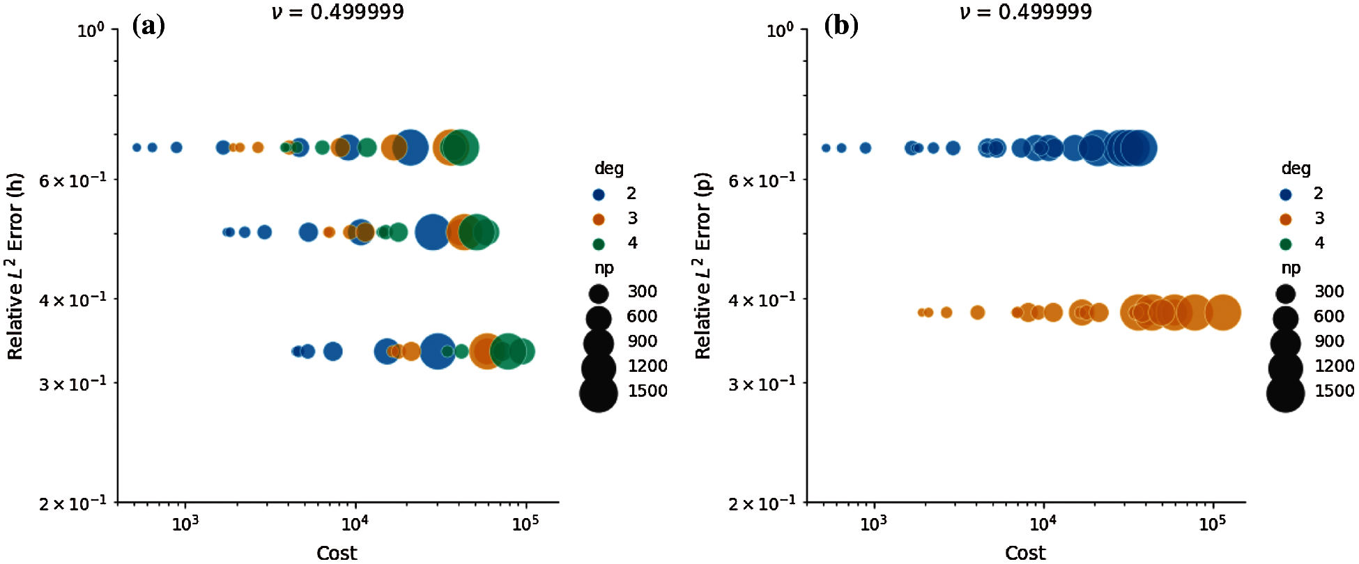
Figure 4: Error vs. cost for nearly-incompressible elastic tube bending. The Pareto optimal configurations occur toward the left region of the plot. Perfect strong scaling occurs when same color dots are collocated. (a) Error based on h-refinement vs. cost. (b) Error based on p-refinement vs. cost

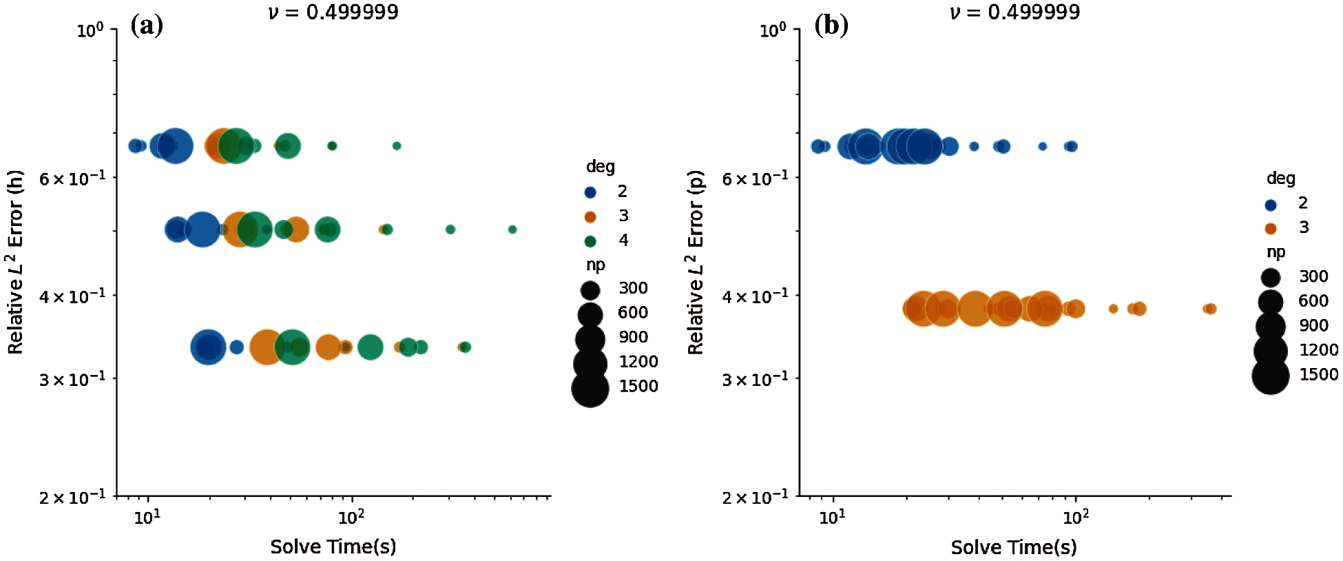
Figure 5: Error vs. time for nearly-incompressible elastic tube bending. The Pareto optimal configurations occur toward the left region of the plot. Perfect strong scaling occurs when same color dots are collocated. (a) Error based on h-refinement vs. time. (b) Error based on p-refinement vs. time

Next, we examine the relative parallel scalability of the matrix-free FE implementation in terms of throughput vs. solve time for p = 1, 2, 3, 4 in the compressible case, and p = 2, 3, 4 in the nearly-incompressible case. Using the tube geometry, new meshes are generated in Trelis. A mesh with 1,638,400 elements is used with polynomial order p = 1. Meshes with 204,800, 60,500, and 25,600 elements are used with polynomial order p = 2, 3, 4, respectively. These mesh sizes in conjunction with polynomial orders p = 1, 2, 3, 4 produce approximately 5.2M DoFs. This problem size is conveniently analyzed in the Pareto diagrams, which roughly occupies one compute node (24 CPU cores) on the parallel platform. For the compressible case, depending on the number of elements, 12, 24, 48, 96, 192, 384, and 768 CPU cores are executed where every problem is run three times for a total of 75 FE simulations. For the nearly-incompressible case, 192, 384, 768, and 1536 CPU cores are called. This resulted in 42 FE simulations for which each problem is run three times. Throughput is computed as millions of DoFs per second per CPU core for each FE simulation. The result of throughput vs. solve time for the compressible and nearly-incompressible cases are presented in Figs. 6a and 6b, respectively. We notice for the compressible case, the implementation scales up to 200–250 CPU cores (Fig. 7a) with polynomial orders 3 and 4. The sub-optimal performance in the code pertains to lack of work amortized to each CPU core for the problem size chosen. However, for the nearly-incompressible case, which is more computationally-intensive compared to the compressible case, the implementation scales up to 800–1000 CPU cores (Fig. 7b) for polynomial orders 2–4 for the problems sizes selected.

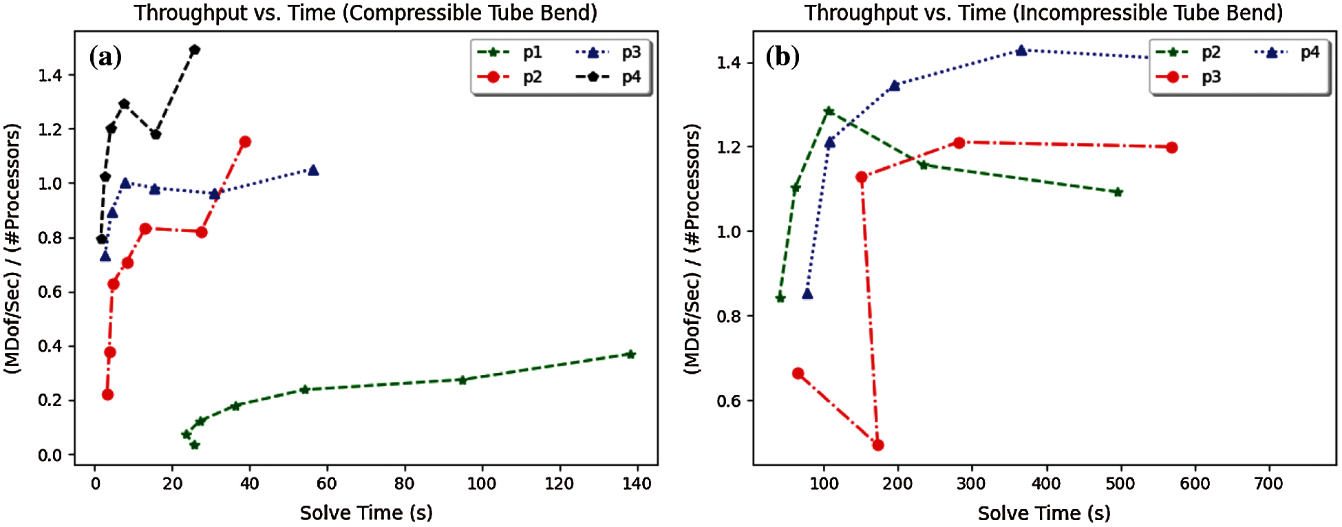
Figure 6: Throughput vs. solve time for compressible and nearly-incompressible elasticity problems. For the problem size with 5.2 M DoFs across polynomial orders p = 1, 2, 3, 4. (a) Throughput vs. solve time. (b) Throughput vs. solve time

In this section, we consider a solid square-cross-section aluminum beam subject to a body force in the negative y direction simulated with p = 1, 2, 3, 4. Fig. 8 shows a coarse structured mesh of the beam. The length of the beam is 5 m, and each side of the square beam cross-section is 0.25 m. The beam is clamped on both ends. A body force of 200 N/m3 is applied in the negative y direction on the beam, which causes the beam to bend 9.1 × 10−4 mm in the negative y direction at the middle of the beam. Fig. 8 shows the deformed mesh of the beam. Similar to the tube bending simulation, the clamped BCs will generate stress concentration (singularity) in the clamped regions. When a stress concentration exists, it can be shown that the order of convergence of the FE solution becomes independent of polynomial order p [32]. That is, the order of convergence of the FE solution cannot be improved by using higher-order finite elements. We investigate this phenomenon by conducting h- and p-refinement with our matrix-free FE implementation in libCEED/PETSc.

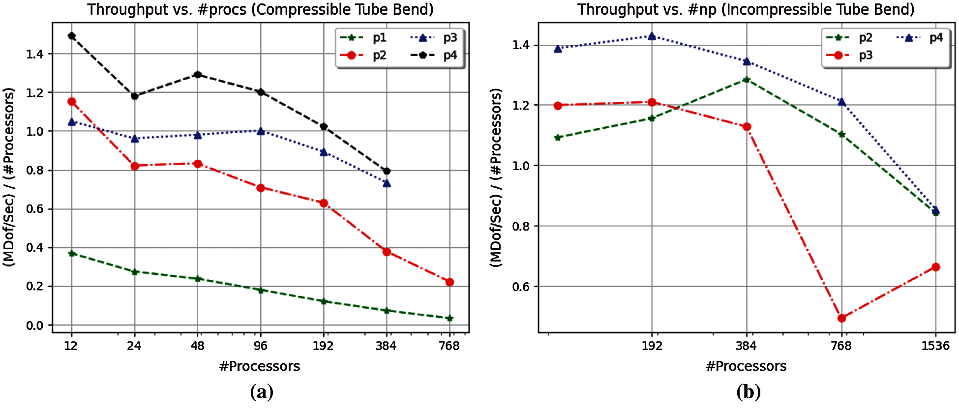
Figure 7: Throughput vs. number of processors for compressible and nearly-incompressible elasticity problems. For the problem size with 5.2 M DoFs across polynomial orders p = 1, 2, 3, 4, the implementation remains scalable up to 200–250 CPU cores in the compressible case with polynomial order 3 and 4, while it is scalable up to 800–1000 CPU cores in the more computationally-intensive nearly-incompressible case. (a) Throughput vs. solve time. (b) Throughput vs. solve time

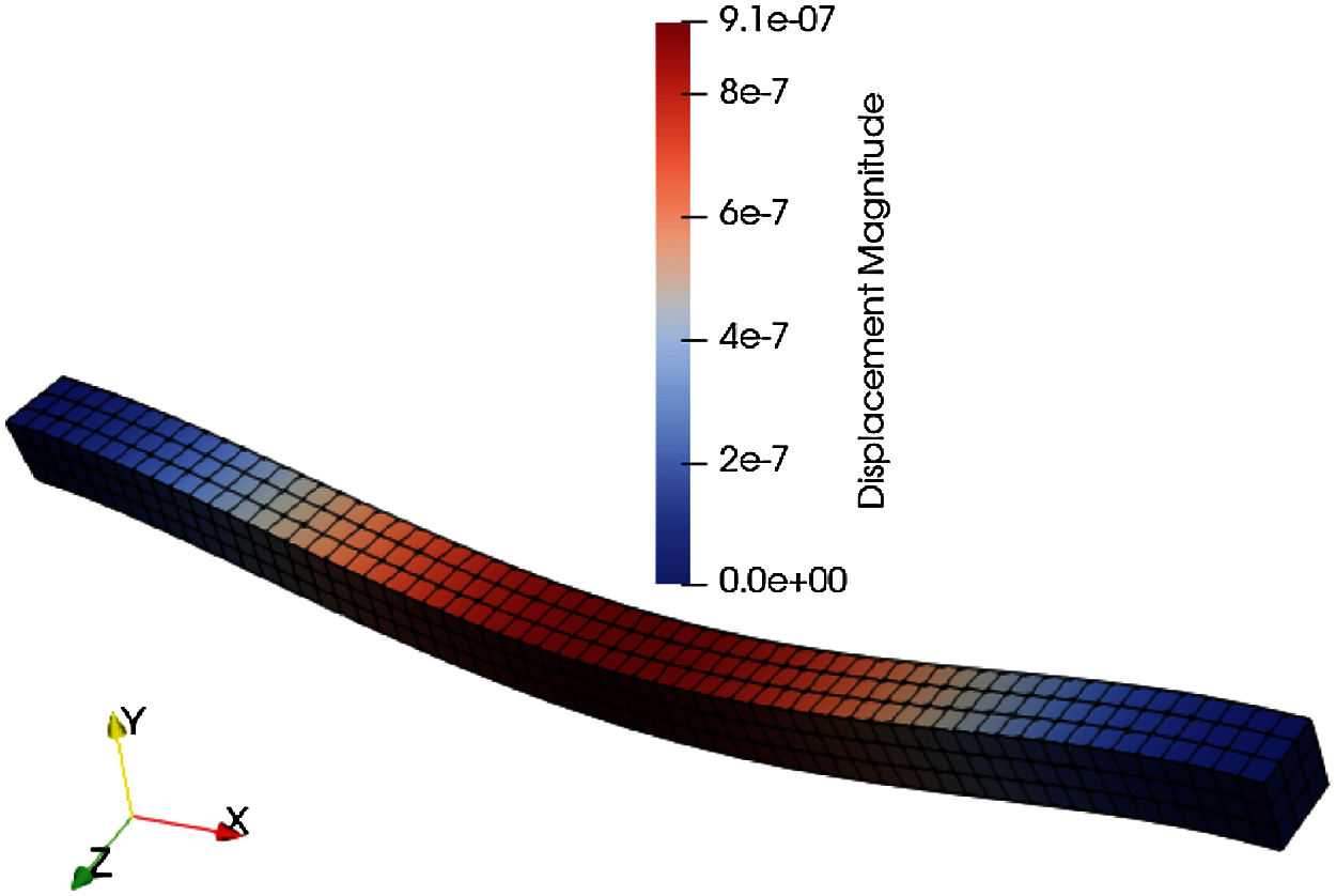
Figure 8: Deformed hexahedral beam structured mesh 5 m in length and square cross-section with side 0.25 m. Beam bent by 200 N/m3 body force in the negative y direction, while the left and right ends are clamped. The body force causes a 9.1 × 10−4 mm displacement in the middle of the beam

Five different refinements of the Hex8 beam mesh are generated with the Trelis software for 558, 4,464, 15,066, 35,712, and 69,750 elements. The finest mesh with 69,750 elements acts as the “exact” solution with respect to strain energy calculation. A total of 60 simulations are conducted where each simulation is repeated 3 times. An L2 strain energy error based on h-refinement per polynomial order is computed for p = 1, 2, 3, 4. In addition, an L2 strain energy error based on higher-order polynomial p for each mesh refinement h is computed. Tables 5a and 5b summarize the refinement (“#Refine”), polynomial degree p (“deg”), number of degrees of freedom (#DoF), strain energy, and the L2 error. The element size for each mesh is computed to be h = 0.1428, 0.0714, 0.0476, 0.0357 m for smallest to largest number of elements mesh, respectively. Fig. 9 represents the h-refinement order of convergence for polynomial orders 1 through 4. The calculated slopes (order of convergence) of the lines that are best fit in the least square sense for polynomial orders p = 1, 2, 3, 4 with h-refinement are 2.43, 2.48, 2.38, and 2.31, respectively. Therefore, we conclude that for this problem the order of convergence of the FE solution on structured meshes with stress concentration (singularity) cannot be improved by using higher-order polynomials. Thus, the lack of optimal spatial convergence with regard to higher-order FE when there is a stress concentration is confirmed, as opposed to when there is no stress concentration (or singularity) [22].

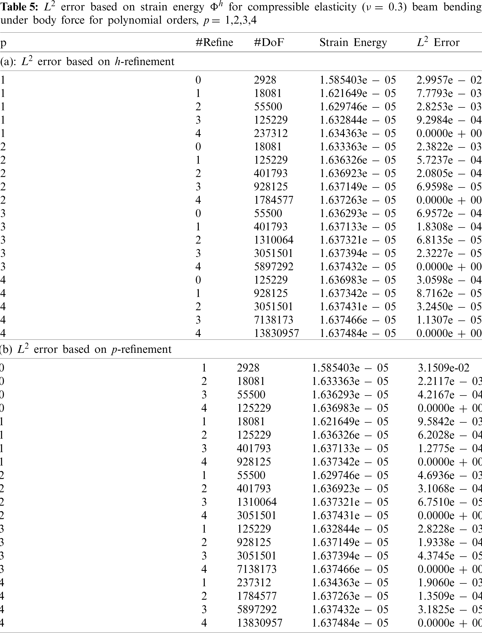
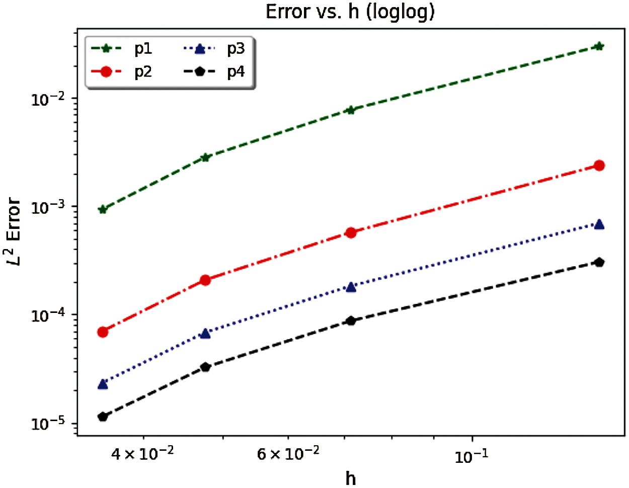
Figure 9: h-refinement order of convergence plot for clamped beam bending under body force with polynomials p = 1, 2, 3, 4

The paper investigated the use of displacement-based higher-order finite elements for compressible and nearly-incompressible linear isotropic elasticity using a matrix-free implementation with p-multigrid preconditioning. It was observed that varying the polynomial order p and mesh size h affects the cost and time it takes to achieve a certain strain energy error for Poisson’s ratios ν = 0.3, 0.499999 in a tube bending problem. Increasing the polynomial order p while fixing the mesh size (h constant) may provide the fastest time to converge to a certain strain energy error between 10−3 and 10−4. However, for strain energy error greater than 10−3, lower-order polynomials may achieve the solution faster. When there is a stress concentration present, higher-order polynomials do not improve the order of convergence in the finite element solution. In addition, polynomial order p = 2 proved to be more efficient than p = 3, 4 for the compressible elastic tube bending problem, which also has a stress concentration (singularity in the stress solution). Each mesh refinement was run with polynomial orders p = 1, 2, 3, 4 for compressible elasticity, and polynomial orders p = 2, 3, 4 for nearly-incompressible elasticity. Using the same mesh refinements h with higher-order polynomials (p = 3, 4) produce a much larger problem size (more DoFs) than when the same meshes are used with polynomial order 2. Therefore, polynomial orders p = 3, 4 appear to be more costly than polynomial order p = 2. An exhaustive search using different polynomial orders p and mesh sizes h may determine if polynomial order p = 2 is truly more cost efficient than polynomial orders p = 3, 4, which will be considered as future work. In addition, for nearly-incompressible elasticity (ν = 0.499999), the tube bending problem could not achieve an error better than 10−1 based on discrete global strain energy Φh computation because of the stress concentration; whereas a smooth method of manufactured solution (MMS) tube problem achieved strain energy error on the order of 10−7, illustrating the difficulty in convergence for h-and p-refinement for near-incompressibility when a stress concentration is present. Therefore, implementing a mixed formulation for handling ν→0.5 appears to be expedient with respect to spatial convergence than solely a displacement-based, higher-order finite element method. Scalability of the matrix-free FEM for compressible elasticity is feasible up to a few hundred CPU cores, while scalability improves for the more computationally-expensive nearly-incompressible case to one thousand CPU cores for the problem sizes chosen in this study. Higher-order finite elements generally still out perform lower-order finite elements within the matrix-free implementation presented in the paper, for which the cost per degree of freedom decreases with increasing p, due to more structured computation and more efficient quadrature.

Notation: Boldface denotes vectors and tensors in symbolic form. Unless otherwise indicated, all vector and tensor products in symbolic form are assumed to be inner products, such as νν=vivi, (ab)ik=aijbjk and (a):(b)=aijbij, where repeated indices denote a sum over those indices. Cartesian coordinates are assumed. The symbol tr(•) is the trace operator, such that tr(σ)=σii. The symbol I is the unit tensor, i.e., Iij=δij, where δij is the Kronecker delta operator, and I is the fourth order identity tensor. p refers to polynomial basis order, h to characteristic element size, d to spatial dimension, and np to number of processors.

Funding Statement: The research relied on computational resources [29] provided by the University of Colorado Boulder Research Computing Group, which is supported by the National Science Foundation (Awards ACI-1532235 and ACI-1532236), University of Colorado Boulder, and Colorado State University.

Conflicts of Interest: The authors declare that they have no conflicts of interest to report regarding the present study.

References

1. Zienkiewicz, O. C., Taylor, R. L., Zhu, J. Z. (2005). The finite element method: Its basis and fundamentals. Amsterdam, Netherlands: Elsevier. [Google Scholar]

2. Hughes, T. J. R. (2000). The finite element method: Linear static and dynamic finite element analysis. Mineola, NY: Dover Publications, Inc. [Google Scholar]

3. Fraeijs de Veubeke, B. (1965). Displacement and equilibrium models in the finite element method. Stress analysis, pp. 145–197. Hoboken, New Jersey: John Wiley & Sons. [Google Scholar]

4. Chiumenti, M., Valverde, Q., de Saracibar, C. A., Cervera, M. (2002). A stabilized formulation for incompressible elasticity using linear displacement and pressure interpolations. Computer Methods in Applied Mechanics and Engineering, 191(46), 5253–5264. DOI 10.1016/S0045-7825(02)00443-7. [Google Scholar] [CrossRef]

5. Nakshatrala, K., Masud, A., Hjelmstad, K. (2008). On finite element formulations for nearly incompressible linear elasticity. Computational Mechanics, 41(4), 547–561. DOI 10.1007/s00466-007-0212-8. [Google Scholar] [CrossRef]

6. Tchonkova, M., Peters, J., Sture, S. (2011). Three-dimensional modeling of problems in poro-elasticity via a mixed least squares method using linear tetrahedral elements. International Journal for Numerical and Analytical Methods in Geomechanics, 35(15), 1656–1681. DOI 10.1002/nag.971. [Google Scholar] [CrossRef]

7. Pian, T. H., Sumihara, K. (1984). Rational approach for assumed stress finite elements. International Journal for Numerical Methods in Engineering, 20(9), 1685–1695. DOI 10.1002/(ISSN)1097-0207. [Google Scholar] [CrossRef]

8. Hughes, T. J., Franca, L. P., Balestra, M. (1986). A new finite element formulation for computational fluid dynamics: V. circumventing the Babuška–Brezzi condition: A stable petrov–galerkin formulation of the stokes problem accommodating equal-order interpolations. Computer Methods in Applied Mechanics and Engineering, 59(1), 85–99. DOI 10.1016/0045-7825(86)90025-3. [Google Scholar] [CrossRef]

9. Sussman, T., Bathe, K. J. (1985). Studies of finite element procedures on mesh selection. Computers & Structures, 21(1–2), 257–264. DOI 10.1016/0045-7949(85)90248-2. [Google Scholar] [CrossRef]

10. Brown, J. (2010). Efficient nonlinear solvers for nodal high-order finite elements in 3D. Journal of Scientific Computing, 45(1–3), 48–63. DOI 10.1007/s10915-010-9396-8. [Google Scholar] [CrossRef]

11. Deville, M. O., Fischer, P. F., Mund, E. H. (2002). High-order methods for incompressible fluid flow, pp. 528. Cambridge: Cambridge University Press. [Google Scholar]

12. Knoll, D. A., Keyes, D. E. (2004). Jacobian-free Newton–Krylov methods: A survey of approaches and applications. Journal of Computational Physics, 193(2), 357–397. DOI 10.1016/j.jcp.2003.08.010. [Google Scholar] [CrossRef]

13. Saad, Y. (2003). Iterative methods for sparse linear systems. 2nd ed. Philadelphia: Society for Industrial and Applied Mathematics. [Google Scholar]

14. Zhu, Y., Sifakis, E., Teran, J., Brandt, A. (2010). An efficient multigrid method for the simulation of high-resolution elastic solids. ACM Transactions on Graphics, 29(2), 16–18. DOI 10.1145/1731047.1731054. [Google Scholar] [CrossRef]

15. May, D., Brown, J., Pourhiet, L. L. (2015). A scalable, matrix-free multigrid preconditioner for finite element discretizations of heterogeneous stokes flow. Computer Methods in Applied Mechanics and Engineering, 290, 496–523. DOI 10.1016/j.cma.2015.03.014. [Google Scholar] [CrossRef]

16. Kronbichler, M., Ljungkvist, K. (2019). Multigrid for matrix-free high-order finite element computations on graphics processors. ACM Transactions on Parallel Computing, 6(1), 1–32. DOI 10.1145/3322813. [Google Scholar] [CrossRef]

17. Rønquist, E. M., Patera, A. T. (1987). Spectral element multigrid. I. Formulation and numerical results. Journal of Scientific Computing, 2(4), 389–406. DOI 10.1007/BF01061297. [Google Scholar] [CrossRef]

18. Vos, P. E., Sherwin, S. J., Kirby, R. M. (2010). From h to p efficiently: Implementing finite and spectral/hp element methods to achieve optimal performance for low-and high-order discretisations. Journal of Computational Physics, 229(13), 5161–5181. DOI 10.1016/j.jcp.2010.03.031. [Google Scholar] [CrossRef]

19. Cantwell, C. D., Sherwin, S. J., Kirby, R. M., Kelly, P. H. (2011). From h to p efficiently: Selecting the optimal spectral/hp discretisation in three dimensions. Mathematical Modelling of Natural Phenomena, 6(3), 84–96. DOI 10.1051/mmnp/20116304. [Google Scholar] [CrossRef]

20. Remacle, J. F., Flaherty, J. E., Shephard, M. S. (2003). An adaptive discontinuous galerkin technique with an orthogonal basis applied to compressible flow problems. SIAM Review, 45(1), 53–72. DOI 10.1137/S00361445023830. [Google Scholar] [CrossRef]

21. Herrmann, L. R. (1965). Elasticity equations for incompressible and nearly incompressible materials by a variational theorem. AIAA Journal, 3(10), 1896–1900. DOI 10.2514/3.3277. [Google Scholar] [CrossRef]

22. Mehraban, A., Thompson, J., Brown, J., Regueiro, R., Barra, V. et al. (2020). Simulating compressible and nearly-incompressible linear elasticity using an efficient parallel scalable matrix-free high-order finite element method. 14th WCCM-ECCOMAS Congress. DOI 10.23967/wccm-eccomas.2020.302. [Google Scholar] [CrossRef]

23. Mehraban, A. (2021). Efficient residual and matrix-free jacobian evaluation for three-dimensional hexahedral finite elements with nearly-incompressible neo-hookean hyperelasticity as applied to soft materials (Ph.D. thesis). University of Colorado Boulder. [Google Scholar]

27. Heys, J., Manteuffel, T., McCormick, S. F., Olson, L. (2005). Algebraic multigrid for higher-order finite elements. Journal of Computational Physics, 204(2), 520–532. DOI 10.1016/j.jcp.2004.10.021. [Google Scholar] [CrossRef]

28. Adams, M., Brezina, M., Hu, J., Tuminaro, R. (2003). Parallel multigrid smoothing: Polynomial vs. Gauss–Seidel. Journal of Computational Physics, 188(2), 593–610. DOI 10.1016/S0021-9991(03)00194-3. [Google Scholar] [CrossRef]

29. Anderson, J., Burns, P. J., Milroy, D., Ruprecht, P., Hauser, T. et al. (2017). Deploying RMACC summit: An HPC resource for the rocky mountain region. Proceedings of the Practice and Experience in Advanced Research Computing 2017 on Sustainability, Success and Impact. New York, NY, USA: Association for Computing Machinery. [Google Scholar]

31. Mahomed, N., Kekana, M. (1998). An error estimator for adaptive mesh refinement analysis based on strain energy equalisation. Computational Mechanics, 22(4), 355–366. DOI 10.1007/s004660050367. [Google Scholar] [CrossRef]

32. Pin, T., Pian, T. H. (1973). On the convergence of the finite element method for problems with singularity. International Journal of Solids and Structures, 9(3), 313–321. DOI 10.1016/0020-7683(73)90082-6. [Google Scholar] [CrossRef]