| Computer Modeling in Engineering & Sciences |
DOI: 10.32604/cmes.2021.016640
ARTICLE
Quantification of Urban Sprawl for Past-To-Future in Abha City, Saudi Arabia
1Department of Civil Engineering, College of Engineering, King Khalid University, Abha, 61411, Saudi Arabia
2Department of Geography, University of Gour Banga, Malda, 732103, India
3Department of Architecture and Planning, College of Engineering, King Khalid University, Abha, 61411, Saudi Arabia
4Department of Geography, Faculty of Natural Sciences, Jamia Millia Islamia, New Delhi, 110025, India
*Corresponding Author: Javed Mallick. Email: jmallick@kku.edu.sa
Received: 14 March 2021; Accepted: 02 July 2021
Abstract: Given that many cities in Saudi Arabia have been observing rapid urbanization since the 1990s, scarce studies on the spatial pattern of urban expansion in Saudi Arabia have been conducted. Therefore, the present study investigates the evidence of land use and land cover (LULC) dynamics and urban sprawl in Abha City of Saudi Arabia, which has been experiencing rapid urbanization, from the past to the future using novel and sophisticated methods. The SVM classifier was used in this study to classify the LULC maps for 1990, 2000, and 2018. The LULC dynamics between 1990–2000, 2000–2018, and 1990–2018 have been analyzed using delta (Δ) change and the Markovian transitional probability matrix. Urban sprawl or urban expansion was modeled using two approaches, such as landscape fragmentation and presence frequency for the first time. The future LULC map for 2028 was predicted using the artificial neural network-cellular automata model (ANN-CA). Future LULC was analyzed using landscape fragmentation and frequency approaches. The results of LULC maps showed that urban areas increased by 334.4% between 1990 and 2018. The Delta change rate showed that 16.34% in urban areas has increased since 1990. While, the transitional probability matrix between 1990 and 2018 reported that the built-up area is the largest stable LULC, having an 83.6% transitional probability value. While 17.9%, 21.8%, 12.4%, and 10.5% of agricultural land, scrubland, exposed rocks, and water bodies were transformed into built-up areas. Urban sprawl models showed that 139 km2 of new urban areas had been set up in 2018, 49 and 69 km2 in 1990 and 2000. Furthermore, in 2018, more than 200% of urban areas were stabilized or became core urban areas. The future LULC map (2028) showed that the built-up area would be 343.72 km2, followed by scrubland (342.98 km2) and sparse vegetation (89.96 km2). The new urban area in 2028 would be 169 km2. The authorities and planners should focus more on the sustainable development of urban areas; otherwise, it would harm the natural and urban environment.
Keywords: Urban sprawl; LULC; landscape fragmentation; cellular automata; SVM; frequency approach
The cities of the world are growing rapidly both in terms of population as well as geographical area [1]. Population growth and economic development are the main drivers of urbanization, especially in developing countries [2,3]. The urban population of the world has already reached 55 percent of the total global population, which is expected to reach about 68 percent by 2050 [4]. Between 1970 and 2000, global urban areas grew fourfold, and by the end of the third decade of the twenty-first century, they are expected to be a third of their original size [5,6]. In Saudi Arabia, the urban population has increased rapidly since 1950. In 1950, the share of the urban population to the total population of the country was about 21 percent, which increased to 58 percent in 1975 and 84 percent in 2018 and is expected to reach about 90 percent by 2050 [7,8]. This rapid growth of the urban population, coupled with industrialization and economic growth, has led to the expansion of urban areas and has created several challenges, such as unplanned growth and congestion [8,9].
The land use land cover change (LULC) due to population growth and urban expansion has increased significantly during the last few decades and is expected to be continuous during the next few decades [10,11]. This unplanned and unprecedented growth of urban areas creates several challenges for planners and policy makers and has negative impacts on the people and the environment [12–14]. Furthermore, rapid urbanization and population growth pose numerous serious threats to urban dwellers and ecosystems, including the formation of urban heat islands (UHI), the formation of micro-climatic zones, biodiversity loss, groundwater depletion, and the degradation of water and air quality [15–18]. One of the major problems originating due to population agglomeration and unplanned growth of cities is urban sprawl [13,19,20]. Urban sprawl refers to the unplanned or less planned expansion of urban areas over less developed or vacant lands on the fringes of urban areas [21,22]. It is a common phenomenon in the cities of developing countries, especially in Asian and African countries [1,23]. Population growth has been identified as the main driving factor of urban sprawl [24]. Further, the factors of urban sprawl have been categorized into two types; direct and potential factors [25]. The direct factors include the expansion of built-up areas, industrial and infrastructural development, whereas the potential factors include natural factors, population and economic growth, government policies and technology [26].
The mapping and monitoring of urban sprawl is important as it leads to the deterioration of the environment and resources, climate change, as well as an increased risk of natural hazards [27–30]. By the application of geospatial techniques, the mapping and monitoring of urban growth and sprawl has become possible [20,31–33]. Attempts have been made to map and monitor urban sprawl and urban spatial growth patterns using landscape matrix [31,34], sprawl matrix [32], Shannon's entropy model, GIS based buffer models etc. Further, studies have been done to model and quantify urban sprawl and LULC changes using the landscape matrix to track the ecological impacts of LULC changes [35–37]. The landscape matrix approach is commonly used to analyze and quantify the structure and pattern of LULC changes and to understand the ecological health of the landscape in the process of urbanization [38–40]. It reduces bias and improves understanding of spatial and temporal changes in landscape patterns [41]. The landscape matrix provides numerical information about urban sprawl. Therefore, it is very difficult to get an idea about which regions have been experiencing new urban areas. However, no studies on the identification and mapping of stages of urban expansion and development have been carried out yet. On the other hand, the landscape fragmentation approach provides different stages of forest and wetland fragmentation [42,43]. It also provides different stages of fragmentation, through which new formations and developed formations can be identified. To overcome the research gap in urban sprawl mapping, we have applied this technique in the present study area to identify new urban areas and stages of urban expansion. The frequency approach [44], on the other hand, has been used in the hydrology field to identify new wetland formation areas based on the frequency of appearance of water pixels in the specific area. Therefore, this method can also be used to identify new urban areas and already developed urban areas.
Numerous studies have been carried out to predict the LULC and urban areas using several methods, such as the Markov chain (MC) [45,46], cellular automata (CA) [47,48], artificial neural network [49], decision trees [50,51], and the Sleuth model [52,53]. The CA model has been frequently utilised for land use change analysis among the many spatio-temporal dynamic modelling methodologies. The CA model has an open structure and may be used in conjunction with other models to anticipate and simulate land use trends. The model has seen considerable use in recent years due to its simplicity, flexibility, and intuitiveness in integrating the spatio-temporal elements of processes. The CA model, on the other hand, has certain quantitative limitations, such as the inability to incorporate driving forces into the simulation process [46], which can be mitigated by combining it with other quantitative models [54]. When the stochastic MC methodology is used with the stochastic CA model, multi-directional LULC change analysis may be simply simulated [55–57]. Many software programmes are available to model the future LULC pattern based on the previous year’s information, including Land Change Modeler, CA-MC, DINAMICA, CLUE-S, and MOLUSCE (Modules of Land Use Change Evaluation) [58,59]. The MOLUSCE-plugin is a QGIS-based tool that was recently released to study and forecast future LULC situations. This plugin can generate a transition probability matrix using the CA-MC method and run simulations using various models such as weights of evidence, logistic regression, artificial neural networks (ANN), multi-criteria evaluation (MCE) [60–62], RF-CA [63], and Fuzzy based integrated model [64,65]. The CA model was utilised to forecast future LULC estimates in the final simulation step [60]. They provided very satisfactory findings. The CA-ANN model is a reliable method for projecting future LULC and plays an important role in land use planning and management. In the present study, we have integrated the ANN model with CA, because the ANN model predicts LULC transitional probability with very high accuracy based on several LULC changing parameters. Based on a highly accurate transitional probability model, CA can easily handle and predict future LULC. For this reason, in the present study, the integrated ANN-CA model has been utilized to predict urban growth.
Previous studies have only concentrated on the LULC mapping and its dynamics analysis using supervised image classification and simple growth rate. But very rare studies have been conducted on the application of machine learning algorithms for mapping LULC and its dynamics analysis using delta (Δ) change and Markovian transitional probability matrix. To the best of the authors’ knowledge, there are no particular techniques for mapping and quantifying urban sprawl and expansion. Many researchers have used Shannon's entropy model, numerical landscape matrix, GIS based buffer analysis, and comparisons between two classified LULC maps for mapping and quantifying urban expansion. But the identification of new urban areas or urban expansion and different stages of urban expansion and stabilization have not been generated from their studies. On the other hand, future prediction of LULC using neural network based cellular automata is not very uncommon, but no studies have been carried out on the modelling of future urban sprawl. Therefore, these research gaps should be addressed to propose proper and very accurate urban development plans. The present study area, Abha, Saudi Arabia, has observed rapid urbanization and conversion of resources providing LULC types to urban areas since 1990. Consequently, there is an urgent requirement to conduct research on urban sprawl modelling and its future situation to monitor and minimize the problems related to urban sprawl. Therefore, to tackle the problems and solve the research gaps, we set five objectives for the present study: First, the LULC mapping for 1990, 2000, and 2018 using the SVM classifier; second, LULC dynamics analysis using delta change rate and transitional probability matrix; third, the urban sprawl and expansion mapping and Quantification using novel geospatial approaches, such as landscape fragmentation and frequency approach; fourth, the future LULC for 2028 prediction using the ANN-CA model; and last, future urban sprawl mapping using the mentioned two novel approaches. The present work is the first comprehensive attempt to provide LULC mapping, urban sprawl mapping, and future LULC and urban sprawl prediction. The main novelties can be summarized as follows:
• General: The work contributes to the robustness of knowledge by applying sophisticated models to an unstudied area of LULC mapping, urban sprawl mapping, LULC future prediction, and future urban sprawl mapping.
• Regional: Increased knowledge of LULC mapping and urban sprawl mapping for the past to the future of Abha City, Saudi Arabia. This is the first attempt in the study area to map LULC and urban sprawl from the past to the future. The outcome of this work would be a valuable basis for urban planners, government authorities, and stakeholders to improve sustainable urban development and management.
• Methodical: Employed SVM and transitional probability matrix for urban mapping and dynamics analysis. Developed novel ways, such as landscape fragmentation and frequency approach, to map urban sprawl and expansion from the past to the future. The ANN-CA model was used to forecast LULC in 2028.
The region selected for this research is the Abha-Khamis Mushayet Twin Cities (Fig. 1) in the South-Western Saudi Arabia. The urban hills are a crucial tourist region with the richest biodiversity of flora and fauna in Asir and KSA [66]. The Twin Cities occupy an area of 1291 km2. It lies between 18°9′33.126″N to 18°30′56.566″N latitude and 42°23′52.477″ E′ to 42°51′42.832″ E longitude. The study area’s topography is undulating, and its elevation varies from 1564 to 2736 m, with a mean of 2102 m at mean sea level. The study area has a heterogeneous terrain and a complex landscape. It is located in an important Afromontane region, where cold and semi-arid climates characterize the city environment [67]. The area of study covers one of the Asir Mountains’ richest and most diverse floristic regions. Jabal Al-Sooda, one of the region’s most famous mountains, is located in the north-western part of the study area, and also has a rich flora. In the study area (Asir Province), the variability in climate and topography has led to the creation of diverse plant species [68]. It has a widespread land loss problem due to anthropogenic activities, high slopes, fragile geology, and rainfall and thus causes ecological imbalances. The twin cities within and surrounding are vulnerable to high-intensity rainfall, and several rural areas undergo flash flooding during the winter season [69,70]. Abha City is the capital city of the Asir region. According to the General Statistics Authority’s 2012 census, the region's population is 289,975, with native Saudis constituting 78 percent of the total population. The twin cities in the Asia region are expecting significant urban transformation and growth, so it is necessary to address a sustainable understanding of urban sprawl and development, which will improve living standards for tourists and residents.
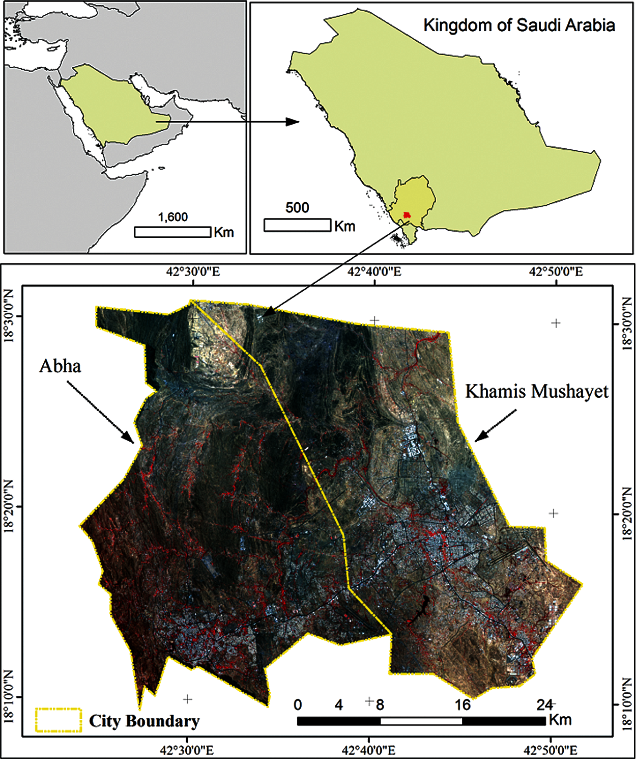
Figure 1: Abha-Khamis Mushyet twin cities selected for this study
The Landsat 4-5 TM and 8 OLI data (path/row: 167/047 and spatial resolution: 30 m) for the years 1990, 2000, and 2018 were downloaded from the USGS Earth Explorer website (https://earthexplorer.usgs.gov). ALOS PALSAR radiometrically terrain corrected (RTC) Digital Elevation Model (DEM) [71] with 12.5 m spatial resolution was acquired from Earth Science Data Systems NASA to extract the topography parameters.
2.3 Methods for LULC Classification
The SVM is a non-parametric machine learning algorithm that classifies the data according to its statistical learning theory [72]. It follows the concept of structural risk minimization (SRM), which separates and maximizes the hyper-plane and data points nearest to the spectral angle mapper (SAM) of the hyper-plane. Further, it divides the data points into several classes using a hyper-spectral plane. In this process, the vectors ensure that the width of the margin will be maximized [73]. The SVM supports multiple continuous and categorical variables and supports linear and non-linear samples in different classes. The training samples that demarcate the margin or hyper-plane of SVM are known as support vectors [74].
In this study, the radial basis function (RBF) kernel SVM algorithm was applied to the LU/LC classification using ENVI 5.3 software. “The SVM was performed using parameters; the kernel width gamma (γ) of 0.143, the penalty parameter (C) of 100, as well as the classification probability threshold value of 0.3”. The classification threshold probability is an important part of the SVM because it unclassifies all rules with probabilities less than the threshold [75]. A value of 0.3 was placed as the threshold to classify all the pixels into a single category. Further, for the pyramid parameter, a value of zero was assigned, which led to the processing of the image at full resolution. The inverse of the number of bands is set by default for the value of gamma. In the present study, eight LULC classes were classified using SVM, such as built up areas, water bodies, dense vegetation, sparse vegetation, agricultural land, scrubland, bare soil, and exposed rock.
In the present study, to explore the LULC dynamics, the post-classification or delta change (cross tabulation) has been employed using the MOLUSCE plug-in in QGIS software [76]. This method is usually been used to quantify and monitor urban sprawl [77]. These post-classification change detection methods are based on pixel to pixel analysis, which calculates the quantity and spatial allocation of LULC changes. Gains and losses of different LULC types can be calculated using delta change and percentage delta change rate.
2.5 Transitional Probability Matrix
To project the LULC change from t to t+1, the Markov model has been employed. It displays the expected number of pixels converted from one LULC type to another over the specified number of time units. The representation of the probabilities is presented in the following matrix p (Eq. (1)):
where p represents the state of probability of transition from i to j.
2.6 Quantification of Urban Sprawl
Several methods have been used for urban sprawl modelling, such as comparisons between two classified images [78], urban sprawl index [32,79], numerical landscape matrices [34], Shannon's entropy [80], GIS based buffer analysis [81]. But these models do not provide the actual quantity of new urban areas and expanded areas. Even so landscape matrices provide numerical information about urban sprawl. Therefore, to model urban sprawl with Quantification and good visuals, two approaches have been employed in the study area. These models were borrowed from hydrological, forest, and wetland studies. These are:
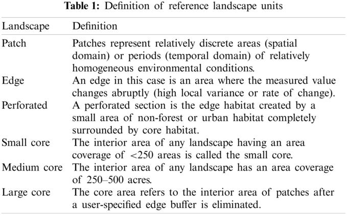
2.6.1 Landscape Fragmentation Approach
Landscape fragmentation (LF) is a process by which large habitat areas are mutilated into smaller and much more isolated habitats [82]. LF is related to the extensive conversion of natural landscapes for human use [83] and has negative effects on biodiversity and ecosystem services also [84]. This process has accelerated in recent years as a result of urbanization and the spread of linear infrastructure such as roads, railways, agricultural land, and so on [85,86]. New discrete urban areas have been formed outside of the main urban areas. Therefore, based on the concentration of urban areas in a particular area, the landscape fragmentation approach has been employed. Six landscape fragmentation indices were prepared, such as patch, edge, perforated, small core, medium core, and large core based on the concentration of urban areas (for details, see Tab. 1) [87]. The higher the concentration of urban areas indicates, the higher the chance of being a core area or stable urban area. The large core indicates a highly concentrated built up area of more than 500 acres, while the medium core has a continuous urban area of 250–500 acres and the small core has a continuous urban area of less than 250 acres. The patch area, on the other hand, denotes a discrete urban region with relatively uniform environmental conditions apart from the core region. The edge is the most dynamic part of the landscape, which can be converted to other land uses easily. The perforated is the core area's surrounding landscape, which could be converted to a small core area in the future. Therefore, patch and edge can be considered as indicators of urban sprawl, while core urban areas have been considered as stable urban areas, which cannot be converted into other land use types. Furthermore, because these landscapes will be stable urban areas in the future, perforated can be a significant indicator of urban area growth.
The Centre for Land Use Education and Research (CLEAR) of the University of Connecticut [88] has launched a GIS tool (Landscape Fragmentation Tool) to demonstrate the fragmentation status of the forest. In the present study, to the best of the author's knowledge, it is the first study to apply the landscape fragmentation approach to identifying urban sprawl.
2.6.2 Urban Presence Frequency
The urban presence frequency was developed in the present study to analyze and map urban sprawl. This model was calculated by following the water presence frequency [44]. This technique has been applied for delineating wetland boundaries and wetland classification [89–91]. The water presence frequency model suggests the average condition of the surface water body of a wetland based on time series data. The model has been generated by averaging the frequency of appearance of water pixels in particular places during the time frame. The higher the frequency of the model indicates, the number of water pixels in those particular places is higher. Those pixels are called stable water pixels, while the lower frequency suggests unstable and new water pixels in those pixels during the time frame. Based on this line of thinking, we have constructed an urban presence frequency. For this, built up areas for different years were extracted from LULC maps. By using Eq. (2), all built-up area maps were combined to create the urban presence frequency map.
where, BPFp is the calculated built up presence frequency for p pixels, Xj is the frequency of jth pixel in image X having an urban appearance, and N is the number of years taken.
2.7 Prediction of Urban Sprawl Using Neural Network Based Cellular Automata
ANN is a machine learning technique that is competent at capturing and representing complex relationships between inputs and outputs. ANN is an interconnected node group inspired by simplifying the brain’s neurons. It contains multiple neurons or nodes, which function simultaneously to transform the data input into output categories. An ANN typically has three layers, namely input, hidden layers, and output. Each layer has several neurons, depending on the particular application in a network. Each neuron is linked by direct links to other neurons in the next consecutive layer. These links reflect the intensity of the output signal [92]. There are many types of networks for an ANN application and the selection of the proper type depends on the nature of the problem and data availability. According to Zhang et al. [93], the multi-layer perception (MLP) is perhaps the most popular network used in hydrological modelling. In MLP, the artificial neurons, or processing units, are arranged in a layered design containing an input layer, a processing (“hidden”) layer (in complex topologies, two hidden layers are used) and an output layer. In the present study, ANN-MLP was used to predict the transitional probability model by integrating land use change conditioning factors. Land use transitional probability conditioning parameters, such as elevation, slope, proximity to urban areas, agricultural land, sparse vegetation, scrubland, and water bodies, were extracted for the 2000 and 2018 LULC maps. The Euclidean distance tool in ArcGIS software 10.5 was then used to construct proximity parameters from the retrieved data. Then, the ANN model was applied to integrate the conditioning parameters for predicting the LULC transitional probability map.
The mathematical explanation of the CA-ANN model has been described below:
Transition rules, restrictions, neighbourhood, and stochastic perturbation are three approaches for obtaining components of restricted CA conceptually. These are incorporated by:
where
The transition rules procedure, which is based on linear regression, is the most important in urban CA modelling (LR). The LR model uses a statistical technique to determine each suitable pixel, in which numerous indications are linearly combined with varying weights. Eqs. (4) and (5) combined show those equations.
where
Furthermore, in our work, the constraint of CA estimation only applies to the urban and non-urban areas (
CA is estimated using 10 * 10 De Moore’s neighbourhood, which is defined as:
where
The probability
where
where
All input variable files should have geographical scales that are the same (i.e., geometry, pixel size, and projection). Within CA modelling, an ANN for transition potential modelling was included. ANNs are a type of machine learning model that is linked to geographical neural networks. This type of integrated CA model is commonly used to compute or approximate nonlinear regression with a large number of input variables [93]. Liu et al. [92] found that the integrated CA-ANN model is particularly well suited to land use change modelling. The benefit of ANNs is that they can link complicated links between input and output data and perform well when modelling with a huge quantity of data. The values of probable transitions for each pixel between the two recorded times were used to create simulations. To correlate to the likelihood of occurrence of estimates for each land variable, the model employed two defined predictors (height and distance from highways). The kappa statistic, which certifies agreement between two categorical datasets, compensated for the predicted differences [94].
In the present study, the whole process has been completed in QGIS software. The QGIS MOLUSCE plug-in has an inbuilt system for collecting training datasets and testing datasets. Based on the training datasets, the ANN model was implemented to generate a land use transitional probability model. During training of the ANN model, several model parameters have to be optimized to get better results. To optimize the ANN model parameters, we have optimized the parameters through a trial and error process. The optimized parameters are: Iteration rate: 1000, Learning rate: 0.001, Momemtum: 0.02, Neighbourhood: 10px, Hidden layer: 10.
After obtaining the transitional probability model by ANN, the prediction of LULC has been conducted by employing CA simulation. It comprises regular spatial lattices of cells. Each cell could have only one of a finite number of states, replying to the states of neighboring cells. It acts on the structure of correlated pixels around one cell. The CA simulation usually comprises multiple iterations to determine whether or not the pixel or cell should be transformed. A preset threshold value has to be set to control the changing rate in order for LULC transformations to occur step by step. If the highest transitional probability of any LULC type is smaller than the threshold value, which is 0.8 in the study based on the trial and error processes, then the pixel or cell stays unconverted. The threshold value ranges from 0 to 1, and 0.8 has been set to keep the LULC conversions stable in each iteration, thus getting fine patterns of simulation. Then, we optimized the CA model. We first set the model to 1 iteration (10 years), indicating the prediction of the upcoming 10 years.
In order to validate the LULC maps and simulated LULC maps, three statistical methods were utilized in the present study area. The statistical techniques are:
The validation of LULC maps is necessary to understand the accuracy level of classified, which was extracted from Landsat satellite imageries [94]. The Kappa coefficient (K) is used to validate the wetland map. K is calculated using Eq. (9).
where, N = total number of pixels; r = number of rows in the matrix; Xii = number of observations in row i and column i; xi+ and x+i are the marginal totals for row i and column i, respectively.
RMSE denotes the square root of the mean squared difference between predicted values through the model and the observed values. RMSE can be employed to quantify the variation of errors in a prediction model and is very effective when massive errors are unwanted [95] The RMSE is cleared by the following formula:
where, Yo indicates the observed value; Yp indicates the predicted value and the number of data points is indicated by the n.
Pearson correlation refers to the assessment of the direction and strength of linear association between two variables, narrating the degree and direction about the most linearly related variable that is associated with one another [96]. It is expressed through this equation:
Here,
LULC maps for 1990, 2000, and 2018 were prepared using the SVM classification technique. The LULC maps were shown in Figs. 2a–2c. The LULC map in the present study area was classified into eight LULC classes, such as built up areas, water bodies, dense vegetation, sparse vegetation, agricultural land, scrubland, bare soil, and exposed rock. Through the visual interpretation of Fig. 2, it can be stated that built up areas have increased significantly during the 1990–2018 periods. Scrubland, on the other hand, has decreased significantly over the last 28 years.
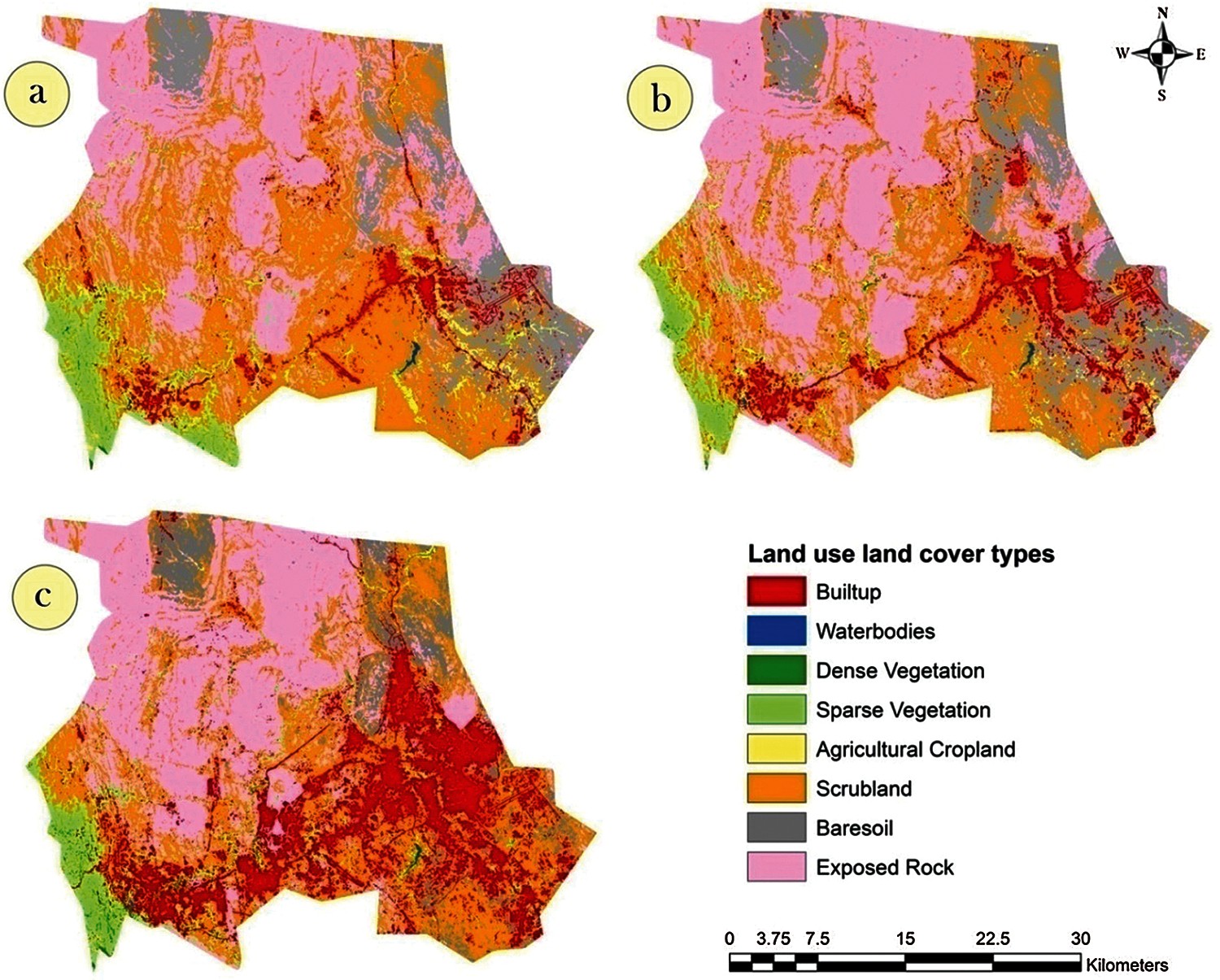
Figure 2: LULC maps for (a) 1990, (b) 2000, and (c) 2018
The area under LULC maps since 1990–2018 was computed and presented in Tab. 1. The built up area showed the largest change in over 28 years. In other words, it was increased noteworthy. The built up area in 2018 was 271.45 km2 in Abha city, compared with 62.46 km2 (1990) and 105.2 km2 (2018) (Tab. 2). In addition, the delta (Δ) change in built up area between 1990 and 2000 was 42.75 km2 (3.34%), which increased to 166.24 km2 (13%) (2000–2018) and 208.99 km2 (16.34%) (1990–2018). The growth rate of built up areas was 334.6% since 1990–2018, signifying noteworthy urban expansion over 28 years. However, the sharp growth has been noticed since 2000 (13% of delta change). This is caused due to rapid and continuous urbanization in the process of development. Scrubland is one of the eight LULC types that has seen a significant decline over 28 years.
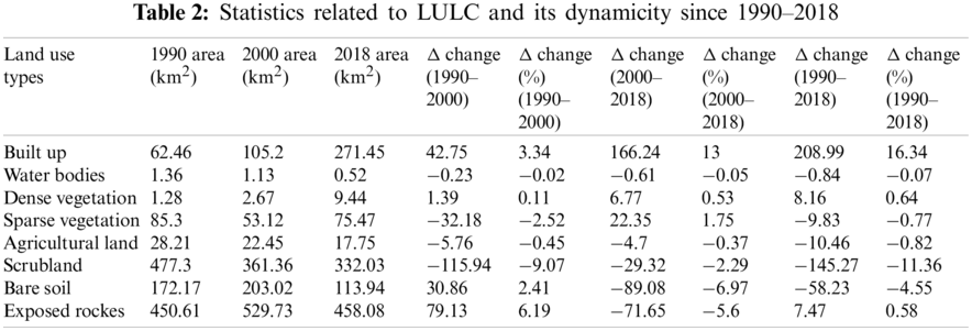
Scrubland covered 477.3 km2 in 1990, but it has shrunk to 332.02 km2 in 2018. The growth rate was −30.38% during the period of 1990–2018. Fig. 2 shows that the built-up area has absorbed the majority of the scrubland. Bare soil also observed some minor loss of about −4% delta change over 28 years, which was converted to urban areas (Tab. 2). On the other hand, other land use types, such as dense vegetation and exposed rocks, observed almost no changes during this period. Although the water body and sparse vegetation experienced minor losses of approximately −0.07% and 0.77% delta change, respectively (Tab. 2). In fact, it can be stated that the scrubland of the study area has observed a very sharp conversion to other land use, especially built up areas, since 2000. One of the main reasons for this land use type's higher conversion rate was its proximity to the main city, as well as its lower elevation (2000 m) and slope (10°) compared to other land use types’ geographical locations.
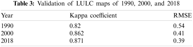
The validation of LULC is a major task, which can not be avoided. Otherwise, the LULC maps’ dependability will be nil. Therefore, in the present study, LULC maps for 1990, 2000, and 2018 were validated with ground truth. The information from the field survey was used to validate the LULC map of 2018, whereas a field survey and a Google Earth image were not available to validate the LUCL maps of 1990 and 2000. As a result, we had to rely on sceondary source. The testing samples were obtained from the blue, shortwave infrared, and near infrared bands of Landsat 4–5tm for the years 1990 and 2000. Based on the collected samples, the kappa coefficient and RMSE were employed to validate the LULC maps statistically. Tab. 3 shows the kappa coefficient and RMSE error for all LULC images. The LULC map of 2018 had a kappa coefficient of 0.871, indicating a very good agreement between ground truth and the LULC map. While the RMSE for the 2018 LULC map was very small. Therefore, it can be concluded that the performance of the LULC classifier for preparing the LULC map for 2018 is highly satisfactory. In addition, the kappa coefficient for LULC maps of 1990 and 2000 was more than 0.8, which suggests good performance. Therefore, the statistical validation analysis suggested that all LULC maps are valid and can be utilized for further research.
3.4 Analysis of LULC Transitional Probability
The trend of LULC change can easily be explored by employing a transitional probability matrix. It indicates the probability of each cell of land use type being converted into other land use types. In the present study, the transitional probability matrix was prepared between the periods of 1990–2000, 2000–2018, and 1990–2018 using the MOLUSE plugin of QGIS following the Markovian approach. Tab. 4 shows the transitional probability matrix between 1990 and 2000. The diagonal bold values showed the probabilities of being unchanged during the period. A zero value indicates that the land has not been converted to other land use types. Exposed rock, bare soil, built-up areas, and water bodies had the highest probability of remaining stable or unchanged, accounting for 86%, 81%, 75%, and 67% of their original areas, respectively (Tab. 4).
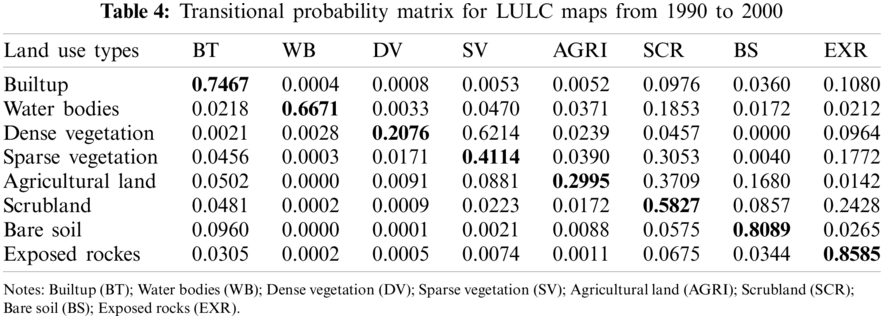
Dense vegetation had the lowest chance of remaining unchanged, with significant areas transformed into sparse vegetation (62.1%) between 1990 and 2000. Sparse vegetation, on the other hand, was converted to scrubland and exposed rocks by 30.5% and 17.7%, respectively, during this period. Similarly, agricultural land was transformed into scrubland and bare soil by 37% and 16.8% respectively. Scrubland was converted to exposed rocks by 24.3%. Therefore, based on the analysis of the transitional proabability matrix, it can be stated that slight land use changes have taken place during this period. Land use types, which can provide services, have transformed into non-resource land use types. This was not a good indicator. Even so, the urbanization process was insignificant, with only 9% of bare land converted to built-up areas.
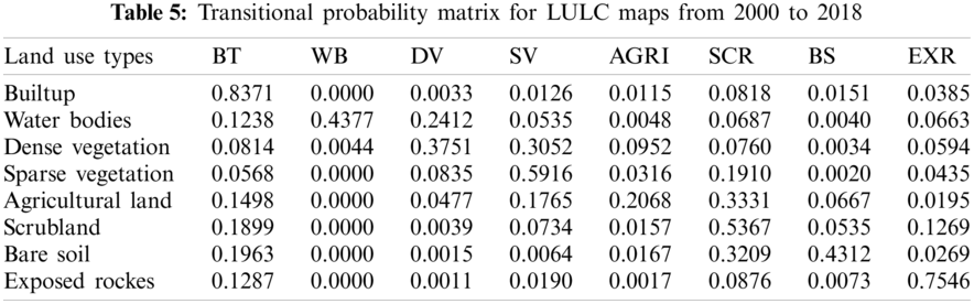
Tab. 5 shows the transitional probability matrix between the LULC maps of 2000 and 2018. Built-up areas, exposed rocks, and sparse vegetation had the highest chances of remaining stable or unchanged during this time period, with 83.7%, 75.4%, and 59.2%, respectively. While, agricultural land had the lowest probability of being transformed by 20.7%. However, very small areas of built up were converted to other land use types, such as exposed rocks (03.8%), scrubland (8.18%), and agricultural land (1.1%). Contrary to this, bare soil, scrubland, agricultural land, exposed rocks, and water bodies were converted to built-up areas by 19.6%, 18.9%, 14.9%, 12.8%, and 12.3% respectively. Except for built up areas, the water bodies did not convert to any other land use types during this period. Similar to built-up areas, scrubland has gained a huge amount of area from other land use types, such as sparse vegetation (19.1%), agricultural land (33.31%), and bare soil (32.09%). From this analysis, it can be concluded that the urbanization process has accelerated to capture other land use types in the process of urbanization and development. Therefore, this period can be called the period of urbanization in the study area.
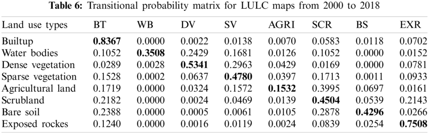
Tab. 6 displays the transitional probability matrix between the LULC maps of 2000 and 2018. Built up areas in the study area were the most consistent and stable land use types, having the largest transitional probability of being unchanged by 83.6%. Similarly, exposed rocks are also a consistent land use type, having a good amount of transitional probability to be unchanged by 75.08%. While, agricultural land was the lowest transitional probability of being unchanged by 15.3% over 28 years. However, built up areas have not changed to other land use types significantly. Scrubland and exposed rocks have gained a negligible amount of built-up area over the last 28 years, increasing by 5.8% and 7%, respectively. In the study area, a fast urbanisation trend has been noticed. Huge amounts of other land use types, such as sparse vegetation, agricultural land, scrubland, bare soil, exposed land, and water bodies, were converted into urban areas by 15.2%, 17.2%, 21.8%, 23.8%, 12.4%, and 19.5%, respectively. Therefore, in the aim of development, urban areas have captured all resources providing land use types, which is not a good sign for the environment and the ecosystem.
3.5 Urban Sprawl Identification Using Landscape Fragmentation
Urbanization and developmental activities have been the key focal point for the conversion of LULC types for over 28 years in the study area. The landscape dynamics analysis also showed that all resource providing land use land types have been transformed into urban areas since 1990–2018 (Tabs. 3–5). Therefore, to control the unscientific and unsystematic expansion of urban areas, the identification of the urban areas in a quantitative and spatial way is an essential task. In the present study, the urban sprawl of Abha city was modelled and quantified by employing landscape fragmentation matrices. Fig. 3 shows the urban sprawl using landscape fragmentation for 1990, 2000, and 2018 based on the arrangement of pixels or concentration of urban areas in a particular area. However, in the present study area, during 1990, the study area had no large core area; while a very small number of small core (4.82 km2) and medium core (2.68 km2) urban areas were observed. But the patch and edge areas were covered by 19.16, and 29.98 km2 respectively. In 2000, the medium core, perforated area of 1990 was converted into a large core area (10.46 km2), while the patch and edge areas increased to 26.03, and 43.88 km2 respectively. Some areas of the edge were transformed into perforated urban areas (13.66 km2). As a result, it can be stated that highly stable urban areas (large core) (10 km2), as well as a large number of new urban areas, were formed between 1990 and 2000, indicating that the urbanization process was carried out both in the center and in nearby rural areas. The urbanization process, which converted different types of LULC to a large extent, was mainly observed in 2018. The patch and edge areas were increased to 40.63, and 98.86 km2. The perforated area was 48 km2. While, the small, medium, and large core areas were covered by 23.19, 8, and 52.76 km2 areas (Fig. 3).
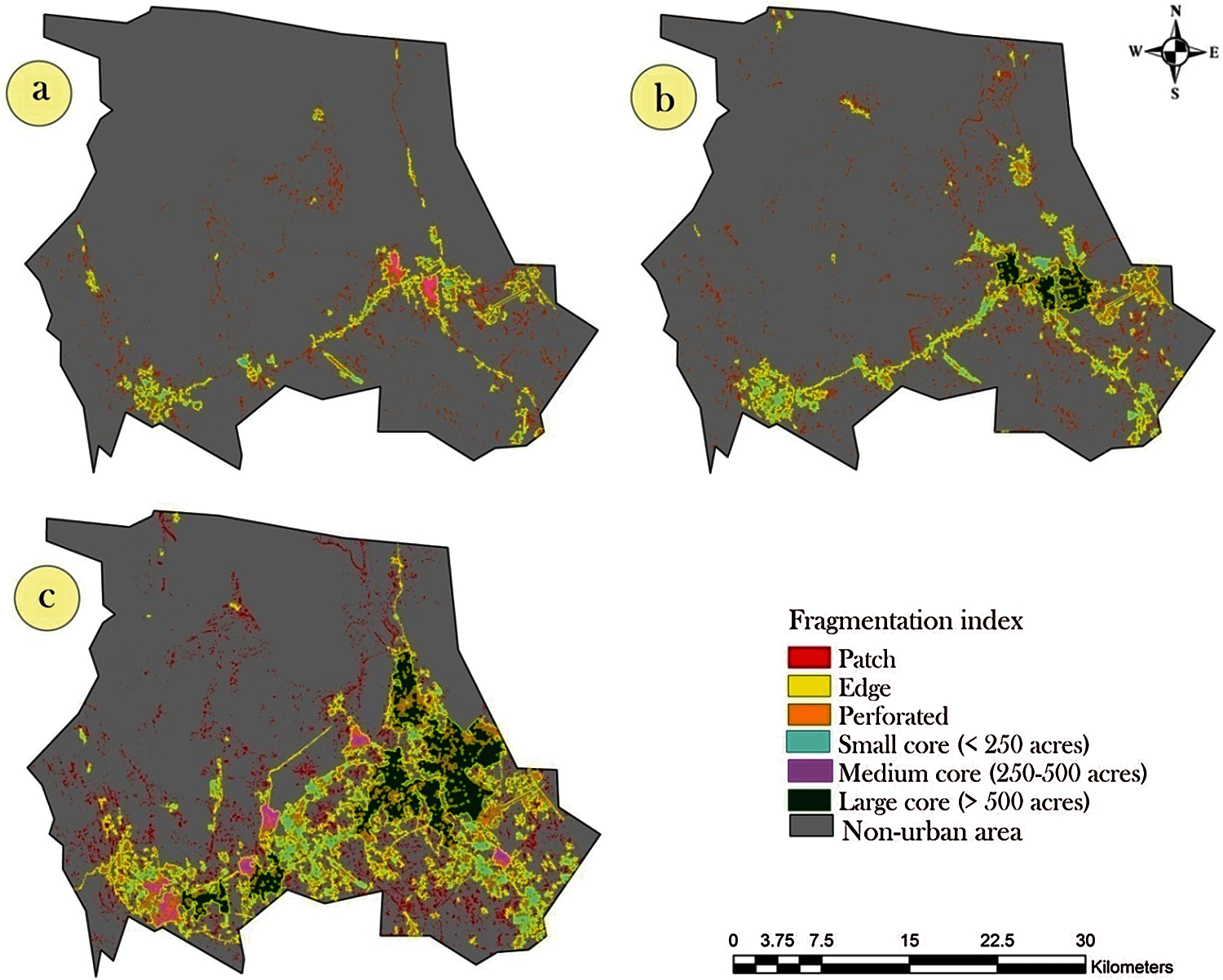
Figure 3: Urban sprawl identification using landscape fragmentation for (a) 1990, (b) 2000, and (c) 2018
Overall, new urban areas (urban sprawl) in the form of patches and edges increased by 111.98% and 229.68% during the last 28 years, which can easily indicate the very fast urbanization process in the study area. The perforated area increased by 728.28%. The stabilized urban area grew by more than 400%. These findings imply that small core, perforated, and some edge areas have been transformed into large cores or stable urban areas. The study area observed an insignificant number of small and medium core areas. As a result, it is possible to forecast that in the future, a large number of stable urban areas will be formed by combining existing perforated, small core, medium core, and some edge areas. According to the trend of horizontal urban expansion, many natural resource-producing land use types will be converted into urban areas as a result of rapid and unsystematic urbanization.
On the other hand, urban sprawl was identified and quantified using built up presence frequency (Fig. 7). Usually, the presence frequency approach is a common approach, which has been employed in wetland studies [44,54]. For the first time, it was utilized in urban science to identify urban sprawl. The idea behind the application of presence frequency is that it can provide information about each pixel, how many times those pixels have appeared in a particular area. Therefore, lower frequencies indicate new pixels or new areas. Based on this line of thinking, it was applied in the study area. Low frequencies indicate new urban areas and vice versa. Fig. 7a shows the urban sprawl modelling using the frequency approach. Over a 28-year period, a 196.35 km2 area was identified as a new urban area. Similarly, the perforated urban area was covered by a 55.78 km2 area. A 43.73 km2 area was designated as the stable area. Therefore, from this analysis, it can be stated that the study area observed huge urban sprawl due to rapid urbanization.
After analyzing the LULC dynamics, the present study was designed to forecast the future LULC of 2028 based on historical LULC maps. Before forecasting future LULC, the important task is to predict the present or existing LULC maps. If the predicted model provides a satisfactory outcome, then the same model can be applied to predict future LULC maps. Prediction of the existing LULC map is an essential task because it is impossible to evaluate the performance of the model for future LULC. As we do not have any idea about the future of LULC, the performance of the model has to be judged before applying it to predicting the future LULC map. Otherwise, the future LULC map would be unreliable. However, the performance of the model can be judged when the model has been applied to predict the existing LULC map. Therefore, in the present study, the LULC map of 2018 was simulated first and evaluated the performance of the model. After obtaining good performance of the model, the LULC map of 2028 was predicted. In the present study, seven LULC change conditioning factors for 2018 and 2028 were identified, such as elevation, slope, proximity to urban areas, agricultural land, scrubland, sparse vegetation, and water bodies. Lower elevations and slopes provide favorable conditions for urban expansion. While regions which are located near urban areas have higher chances of being converted to urban areas. In contrast, high distances from core forest, water bodies, and agricultural land have been deciding factors in urban area transformation. Figs. 4 and 5 show the LULC change conditioning factors for 2018 and 2028. The conditioning factors for predicting 2018 were prepared from the data of 2000, while the conditioning factors for predicting 2028 were generated from the data of 2018. However, Fig. 4 showed that the eastern and north eastern parts of the study area have lower elevation and slope, which is a suitable condition for constructing new habitat. While the northern part of the study area was very far from the existing urban area (6270 m in 2000 and 7068 m in 2018). Therefore, the conversion to an urban area in this region is very difficult, even in the future. On the other hand, agricultural land, sparse vegetation, and scrubland in the eastern and north eastern parts of the study area were situated very close to urban areas in 2000. Therefore, these areas had a higher chance of being converted to urban areas in 2018. Similarly, the closeness of these areas to urban areas increased significantly in 2018, which indicates the conversion of these areas to urban areas in 2028 (Fig. 5). Then, the ANN-MLP model was applied to integrate these parameters to construct a land use suitability model for predicting 2018 and 2028.
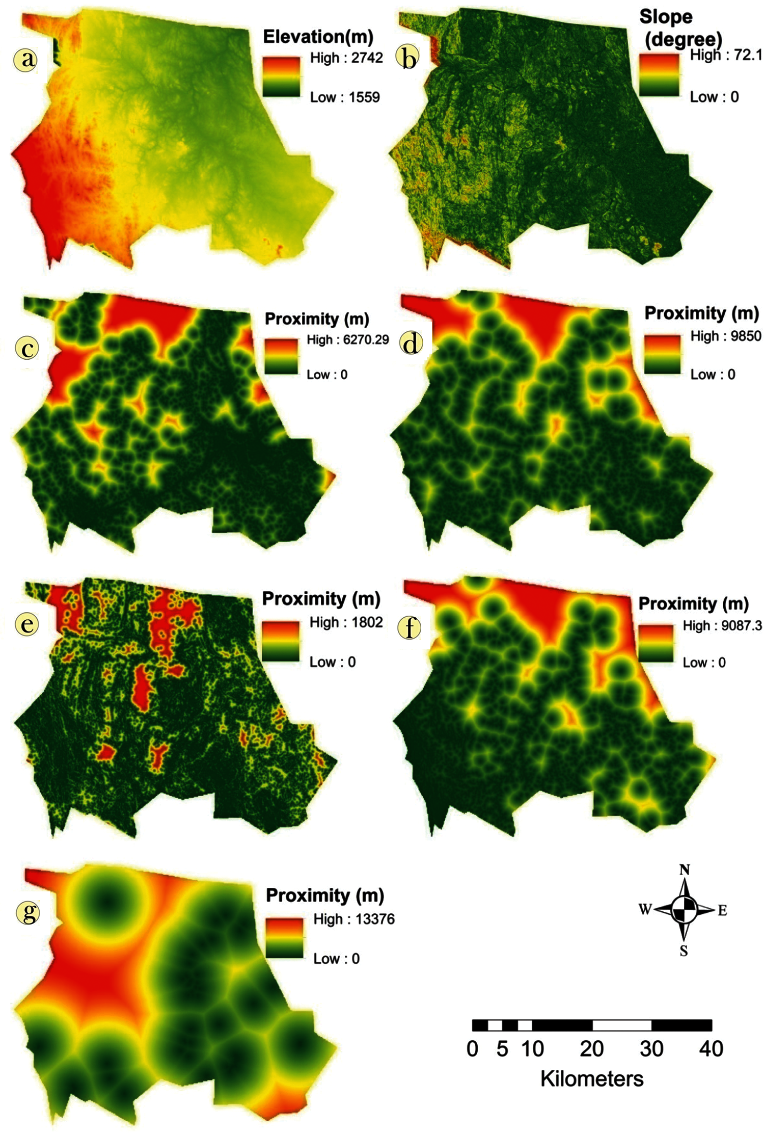
Figure 4: LULC change conditioning factors, such as (a) elevation, (b) slope, (c) proximity to urban area, (d) proximity to agricultural land, (e) proximity to scrubland, (f) proximity to sparse vegetation, (g) proximity to water bodies for predicting 2018 LULC
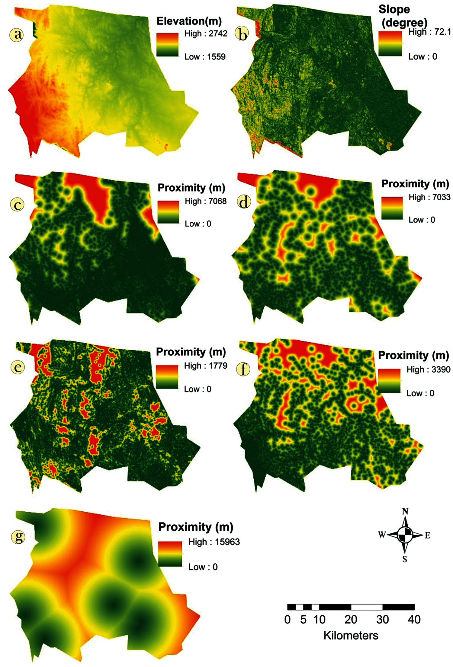
Figure 5: LULC change conditioning factors, such as (a) elevation, (b) slope, (c) proximity to urban area, (d) proximity to agricultural land, (e) proximity to scrubland, (f) proximity to sparse vegetation, (g) proximity to water bodies for predicting 2028 LULC
Based on the ANN model based land suitability model, the CA model was implemented to construct the LULC maps of 2018 and 2028. After obtaining the LULC map in 2018, it was matched with the original LULC map to judge the performance of the ANN-CA model for prediction. The correction of prediction, correlation coefficient and kappa coefficient for the LULC map of 2018 were 76.2%, 0.841 and 83%, which indicates satisfactory performance of the model. After validation of the predicted LULC map of 2018, the LULC map of 2028 was constructed using the same model. No model parameters were changed during the modelling procedure of 2028 to avoid different outcomes of the model. Fig. 6 shows a simulated LULC map of 2018 and a predicted LULC map of 2028.
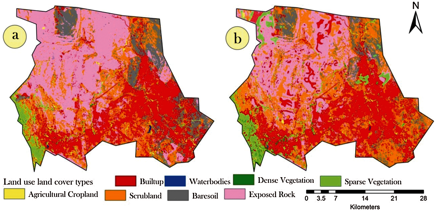
Figure 6: LULC simulation and prediction for (a) 2018, and (b) 2028
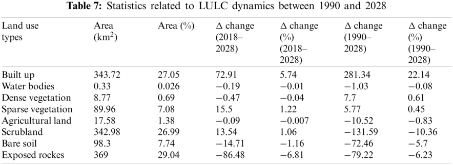
Tab. 7 shows the land use dynamics of LULC from 1990 to 2028. It showed that the built up area would be 343.72 km2, which will increase by 281.34 km2 (22.14%) and 72.91 km2 (5.74%) compared to the LULC maps of 1990 and 2018. The area under bare soil has decreased by 14.71 km2 since 2018 and 72.46 km2 since 1990. The exposed rock has decreased by 86.48 km2 since 2018 and 79.22 since 1990. Other land use types in 2028 would remain quite similar to the LULC of 2018.
3.7 Future Urban Sprawl Modelling
Based on the future LULC maps of 2028, it can be seen that urban areas or built up areas will increase by 26.79% since 2018. Therefore, the new urban areas would obviously be increased. In the present study, urban sprawl was modeled using both the frequency approach and the landscape fragmentation approach (Figs. 7b and 7c).
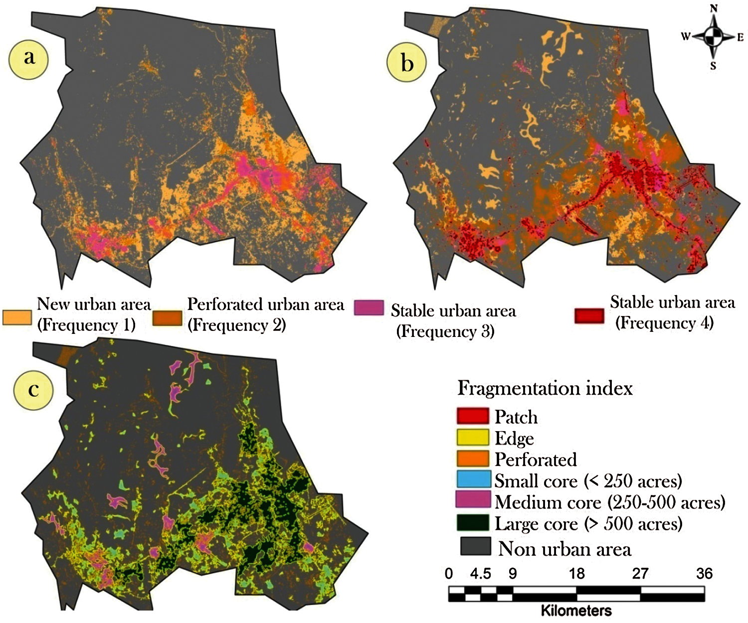
Figure 7: Urban sprawl using frequency approach (a) 1990–2018, (b) 1990–2028, and landscape fragmentation approach (c) 2028
The new urban area would cover 108.1 km2, while the perforated urban area would cover 172.67 km2. The urban areas that are stable and highly stable would be 52.18 and 43.24 km2, respectively. If the authorities were notable to control the unsystematic, very fast urbanization, in the future, many resources providing land use types could be transformed into new urban areas. Urban sprawl can be identified more clearly using the landscape fragmentation approach. Fig. 7c showed that new urban areas in the form of patches and edges would be 39.91 km2 and 120.78 km2. While the perforated urban area would be 60.84 km2. In 2028, the stable urban areas of various sizes, such as small core, medium core, and large core areas, would be 28.19, 20.86, and 73.57 km2 (Fig. 7c). Between 1990 and 2028, the growth rate of new urban areas (patch and edge) would be 108.26% and 302.79%, respectively. In addition, perforated urban areas would increase by 949.83%. The stabilized urban area would grow by more than 450%. As a result, it can be stated that in the future, the urbanization process will be faster and more stable in the center. It does not imply that horizontal expansion or urban sprawl will be reduced. The expansion of new urban areas would be less than that of the stabilized part. Stable urban areas would be more compact and overpopulated or crowded in 2028. Authorities should focus on this to control horizontal expansion towards both the outside and inside of the city. Otherwise, in the future, the natural environment as well as the urban environment would be in danger.
The current study investigated how to forecast and quantify urban spread in Abha, Saudi Arabia, between 1990 and 2028. From the following three perspectives, this study contributes to the existing literature on urban area extension and sprawl modelling utilising geospatial technology: First, we used the delta change and transitional probability matrix to map spatiotemporal LULC maps and investigate land use dynamics; second, urban sprawl from 1990 to 2018 was identified using new approaches such as landscape fragmentation and frequency approach; and third, future land use for 2028 was predicted using the ANN-CA model and future urban sprawl was explored using the two new approaches. Three significant findings have emerged from our research. First, significant LULC dynamics have been found in Abha between 1990 and 2018. However, there was no notable change in LULC in the city between 1990 and 2000. Following the year 2000, the study area underwent a transformation as a result of the development activities. As a result, between 2000 and 2018, significant LULC dynamics were detected. Due to the fast urbanisation and modernisation of the study area, a large amount of horizontal urban growth was seen during this time. Agricultural land, scrubland, and topographically suitable unoccupied places have all been used to create new urban areas. Several Saudi Arabian cities, including AlRiyadh city (increased by 545 km2 between 1987 and 2017), Riyadh (increased by 185% between 1990 and 2014), Al-Khobar City (increased by 110% between 1990 and 2001), Jeddah (increased by 109.76 km2 between 1972 and 2014), and Al Hassa oasis (increased by 254.52 km2 between 1972 and 2014), have observed substantial growth [97–101]. Apart from Saudi Arabia, Dewan et al. [102] observed that the urban area of Dhaka megacity rose by 190% between 1975 and 2003, which is similar to our findings. Between 1972 and 2018, the built-up area in Mangalore, India, rose by 39%, according to Dhanaraj et al. [103]. According to Badlani et al. [104], the urban area of Gandhinagar, India, has grown by 73 percent in 26 years (1989–2015). According to Sahana et al. [32], the urban area of the Kolkata urban agglomeration rose by 24.5 percent between 2000 and 2015, with agricultural land being converted (decreased by 66.9 percent between 2000 and 2015). According to Altuwaijri et al., [97], the population of AlRiyadh has expanded by 600 percent in the previous four decades. This pattern has been detected in several researches all across the world [105–114].
Second, between 1990 and 2028, the creation of new urban areas on agricultural land and scrubland increased significantly in Abha. Along with urban growth, the study area witnessed the urban area's stabilisation process in certain locations. The number of rapidly changing metropolitan regions that will become stable in the near future has also grown dramatically. Many cities across the world, including Bilwara (Rajsthan, India), Mansoura (Egypt), Hangzhou (China), Harbin (China), Khoms (Libya), and 417 metropolitan areas (Europe), have had difficulties with unsystematic urban expansion, similar to our results [115–120]. Another intriguing aspect of this research is the use of landscape fragmentation and frequency approaches to identify urban sprawl rather than traditional methods. Urban sprawl identification is a challenging but necessary undertaking for urban management [121]. To determine urban sprawl in Kolkata’s agglomeration region, Sahana et al. [32] analysed two LULC maps at two distinct dates. By comparing two LULC maps, Bhat et al. [78] were able to detect urban sprawl in Dehradun, India. By comparing two classed LULC maps, El Garouani et al. [122] detected urban sprawl in Fez, Morocco. In Tshwane, South Africa, Magidi et al. [34] employed landscape matrices to identify urban sprawl. Mosammam et al. [80] used Shannon's entropy model to find urban sprawl in the Iranian city of Qom. In Beijing, China, Yang et al. [81] employed GIS-based buffer analysis to identify urban growth. To identify urban sprawl, many studies analysed two LULC maps from different times [32,123,124]. These methodologies are unable to quantify the extent of urban sprawl, particularly how many additional urban areas exist. The use of a landscape fragmentation and frequency technique not only provides valuable Quantification of the urban region, but also excellent visualisation. As a result, urban sprawl and even the stages of urbanisation may be detected from a bird’s eye view. These techniques have a relatively basic modelling method, yet they provide extremely reliable results. As a result, urban planners, city officials, and scientists may use these methodologies to mimic urban sprawl when developing urban and environmental management strategies.
Third, we calculated that the urban growth in 2028 will be 343.72 km2, with a delta change rate of 22.14 percent since 1990. In the current study area, the growth rate since 1990 has been 450.3%. This rate of urbanisation is regarded to be extremely fast. Many cities in the Arab world, such as Al Riyadh, Tabriz, Iran (raised by 116% in 2035), Nizwa, Al Dakhliyah, and Oman, Iran (up by 418.5% in 2038), have witnessed the same growth rate for the future [97,125,126]. The cause of this remarkable growth rate is the rapid expansion of infrastructural infrastructure in the metropolitan region as a result of modernization [126]. Rural migration has thus grown quite quickly in the hunt for work and other conveniences. Rural migrants began to settle in the vicinity of metropolitan centres. Many Saudi Arabian towns have thus seen quite exceptional urban expansion. The current study area has an urban development rate equivalent to that of India and China, which are highly rapidly developed. Both emerging countries have had very rapid urban expansion worldwide. The overcrowding in both nations is one of the key reasons. While overpopulation is not a major issue in Saudi Arabia, the country has experienced increasing urbanisation as a result of urban-centric growth and possibilities. However, the urbanisation process will be extremely difficult in the near future due to the conversion of natural resource-providing land use types and overcrowding. As a result, it would wreak havoc on the natural and urban environments.
Above all, the identification of urban sprawl using a landscape fragmentation and frequency method is a significant contribution to the literature on urban sprawl. Even little researche on future urban sprawl mapping has been conducted. In the current study, the future urban sprawl was identified using the two methodologies indicated. Because urban sprawl has become a worldwide issue or worry in recent decades, there is little doubt that the fragmentation methodologies utilised in this study may be used for the assessment of urban development in other cities and nations [124,127]. Furthermore, this study offers a thorough examination of spatiotemporal LULC mapping, as well as analyses of its dynamics using the Markovian transitional probability matrix, urban sprawl identification using novel approaches, future LULC modelling using the ANN-CA model, and future urban sprawl identification. As a result, the outcomes of this study will aid in raising awareness of the alarming severity of urban land growth. Policymakers may use the data to establish strategies to reduce urban sprawl by restricting rural-urban migration, LULC conversions, and implementing more compact urban development policies [26,32,121,125,128,129,130].
The goal of this research was to give a complete examination of LULC trends from 1990 to 2018. Since 1990, the built-up area has expanded by 16.34 percent, compared to 3.34 percent between 1990 and 2000 and 13 percent between 2000 and 2018. After the year 2000, urbanization development accelerated. Between 1990 and 2018, the transitional probability matrix analysis revealed that the most stable LULC type in the study area is urban, with a transitional probability of 83.6 percent. Agricultural land, scrubland, exposed rocks, and water bodies, on the other hand, were converted to built-up areas by 17.9%, 21.8%, 12.4, and 10.5, respectively. Agricultural land, on the other hand, was the most transformed land use. Scrubland, built-up areas, and sparse vegetation acquired 39.9%, 17.1%, and 15.72% of agricultural land. Over the course of 28 years, new urban areas in the form of patches and edges rose by 111.9 percent and 229.6 percent, respectively, according to the current study. In 2018, more than 200 percent of urban areas were stabilized or converted to core urban areas. The LULC map for 2028 was also projected using the ANN-CA model. The results of the ANN-CA were satisfactory. According to the LULC of 2028, the built-up area expanded to 343.72 km2, while bare soil and exposed rocks decreased by 86.48 and 14.71 km2, respectively. In 2028, the area covered by agricultural land decreased significantly. The data gathered in the study area allows for a thorough examination of urban sprawl and its dynamics, which might be useful in planning for long-term urban growth.
Of course, the use, of course, resolution satellite images (Landsat) for LULC mapping utilizing a supervised image classification approach is a key drawback of this study. Due to a lack of socioeconomic data, which impacts land use changes, the prediction model's performance may be low. For forecasting LULC in 2018 and 2028, we employed a lower number of explanatory factors. High-resolution images, such as SPOT-5, KOMPSAT series, IKONOS, QUICKBIRD, and others, would be highly beneficial for obtaining very high precision urban growth and sprawl mapping. The management plans will be highly accurate since they may supply very minute details of LULC types. Deep learning approaches such as artificial neural networks, and random forests, on the other hand, can categorize LULC types more accurately than SVM. Similarly, we have just integrated ANN with CA for the prediction of LULC. Instead of it, Resnet, Xception, and VGG Net can perform better results for forecasting. Finally, to build high-quality future LULC maps, the number of variables should be raised. By resolving these issues, the work will be more robust and thorough, which will aid in the development of thorough and accurate urban and natural resource management plans.
Acknowledgement: Authors thankfully acknowledge the Deanship of Scientific Research for proving administrative and financial supports and NASAUSGS personnel at the land DAAC provided the latest Landsat satellite image was greatly appreciated.
Funding Statement:Funding for this research was given under Award No. R.G.P2/75/41 by the Deanship of Scientific Research; King Khalid University, Ministry of Education, Saudi Arabia.
Conflicts of Interest: The authors declare that they have no conflicts of interest to report regarding the present study.
1. Chen, M., Zhang, H., Liu, W., Zhang, W. (2014). The global pattern of urbanization and economic growth: Evidence from the last three decades. PLoS One, 9(8), e103799. DOI 10.1371/journal.pone.0103799. [Google Scholar] [CrossRef]
2. Jarah, S., Zhou, B., Abdullah, R., Lu, Y., Yu, W. (2019). Urbanization and urban sprawl issues in city structure: A case of the Sulaymaniah Iraqi Kurdistan Region. Sustainability, 11(2), 485. DOI 10.3390/su11020485. [Google Scholar] [CrossRef]
3. Wu, Y., Li, S., Yu, S. (2016). Monitoring urban expansion and its effects on land use and land cover changes in Guangzhou city. China Environmental Monitoring and Assessment, 188(1), 1–15. DOI 10.1007/s10661-015-5069-2. [Google Scholar] [CrossRef]
4. United Nations, Department of Economic and Social Affairs, Population Division (2019). World Urbanization Prospects: The 2018 Revision (ST/ESA/SER.A/420). New York: United Nations. [Google Scholar]
5. Seto, K. C., Fragkias, M. (2005). Quantifying spatiotemporal patterns of urban land-use change in four cities of China with time series landscape metrics. Landscape Ecology, 20(7), 871–888. DOI 10.1007/s10980-005-5238-8. [Google Scholar] [CrossRef]
6. Seto, K. C., Güneralp, B., Hutyra, L. R. (2012). Global forecasts of urban expansion to 2030 and direct impacts on biodiversity and carbon pools. Proceedings of the National Academy of Sciences of the United States of America, 109(40), 16083–16088. DOI 10.1073/pnas.1211658109. [Google Scholar] [CrossRef]
7. Alahmadi, M., Atkinson, P. M. (2019). Three-fold urban expansion in Saudi Arabia from 1992 to 2013 observed using calibrated DMSP-OLS night-time lights imagery. Remote Sensing, 11(19), 2266. DOI 10.3390/rs11192266. [Google Scholar] [CrossRef]
8. Ministry of Municipal and Rural Affairs (2019). Saudi cities report. Future Saudi cities programme. King Fahd National Library Cataloging-in-Publication. [Google Scholar]
9. Belloumi, M., Alshehry, A. (2016). The impact of urbanization on energy intensity in Saudi Arabia. Sustainability, 8(4), 375. DOI 10.3390/su8040375. [Google Scholar] [CrossRef]
10. Ahmed, H. A., Singh, S. K., Kumar, M., Maina, M. S., Dzwairo, R. et al. (2020). Impact of urbanization and land cover change on urban climate: Case study of Nigeria. Urban Climate, 32(2), 100600. DOI 10.1016/j.uclim.2020.100600. [Google Scholar] [CrossRef]
11. Fang, S., Gertner, G. Z., Sun, Z., Anderson, A. A. (2005). The impact of interactions in spatial simulation of the dynamics of urban sprawl. Landscape and Urban Planning, 73(4), 294–306. DOI 10.1016/j.landurbplan.2004.08.006. [Google Scholar] [CrossRef]
12. Li, B., Shi, X., Wang, H., Qin, M. (2020). Analysis of the relationship between urban landscape patterns and thermal environment: A case study of Zhengzhou city. China Environmental Monitoring and Assessment, 192(8), 1–13. DOI 10.1007/s10661-020-08505-w. [Google Scholar] [CrossRef]
13. Bhat, P. A., ul Shafiq, M., Mir, A. A., Ahmed, P. (2017). Urban sprawl and its impact on landuse/land cover dynamics of Dehradun City, India. International Journal of Sustainable Built Environment, 6(2), 513–521. DOI 10.1016/j.ijsbe.2017.10.003. [Google Scholar] [CrossRef]
14. Wentz, E., Anderson, S., Fragkias, M., Netzband, M., Mesev, V. et al. (2014). Supporting global environmental change research: A review of trends and knowledge gaps in urban remote sensing. Remote Sensing, 6(5), 3879–3905. DOI 10.3390/rs6053879. [Google Scholar] [CrossRef]
15. Wang, S., Gao, S., Li, S., Feng, K. (2020). Strategizing the relation between urbanization and air pollution: Empirical evidence from global countries. Journal of Cleaner Production, 243(4), 118615. DOI 10.1016/j.jclepro.2019.118615. [Google Scholar] [CrossRef]
16. Roy, S. S., Rahman, A., Ahmed, S., Shahfahad, Ahmad, I. A. (2020). Alarming groundwater depletion in the Delhi Metropolitan region: A long-term assessment. Environmental Monitoring and Assessment, 192(10), 1–14. DOI 10.1007/s10661-020-08585-8. [Google Scholar] [CrossRef]
17. Sultana, S., Satyanarayana, A. N. V. (2019). Impact of urbanisation on urban heat island intensity during summer and winter over Indian metropolitan cities. Environmental Monitoring and Assessment, 191(3), 1–17. DOI 10.1007/s10661-019-7692-9. [Google Scholar] [CrossRef]
18. Mallick, J., Rahman, A., Singh, C. K. (2013). Modeling urban heat islands in heterogeneous land surface and its correlation with impervious surface area by using night-time ASTER satellite data in highly urbanizing city, Delhi-India. Advances in Space Research, 52(4), 639–655. DOI 10.1016/j.asr.2013.04.025. [Google Scholar] [CrossRef]
19. Shao, Z., Sumari, N. S., Portnov, A., Ujoh, F., Musakwa, W. et al. (2020). Urban sprawl and its impact on sustainable urban development: A combination of remote sensing and social media data. Geo-spatial information science. UK: Taylor & Francis. [Google Scholar]
20. Rahman, A., Aggarwal, S. P., Netzband, M., Fazal, S. (2011). Monitoring urban sprawl using remote sensing and GIS techniques of a fast growing urban centre. India IEEE Journal of Selected Topics in Applied Earth Observations and Remote Sensing, 4(1), 56–64. DOI 10.1109/JSTARS.2010.2084072. [Google Scholar] [CrossRef]
21. Dinda, S., Das, K., Chatterjee, N. D., Ghosh, S. (2019). Integration of GIS and statistical approach in mapping of urban sprawl and predicting future growth in Midnapore town. India Modeling Earth Systems and Environment, 5(1), 331–352. DOI 10.1007/s40808-018-0536-8. [Google Scholar] [CrossRef]
22. Bhatta, B. (2010). Urban growth and sprawl. Analysis of urban growth and sprawl from remote sensing data, pp. 1–16. Berlin, Heidelberg: Springer. [Google Scholar]
23. Yue, W., Liu, Y., Fan, P. (2013). Measuring urban sprawl and its drivers in large Chinese cities: The case of Hangzhou. Land Use Policy, 31(4), 358–370. DOI 10.1016/j.landusepol.2012.07.018. [Google Scholar] [CrossRef]
24. Fertner, C., Jørgensen, G., Sick Nielsen, T. A., Bernhard Nilsson, K. S. (2016). Urban sprawl and growth management–drivers, impacts and responses in selected European and US cities. Future Cities and Environment, 2, 9. DOI 10.1186/s40984-016-0022-2. [Google Scholar] [CrossRef]
25. Barrington-Leigh, C., Millard-Ball, A. (2015). A century of sprawl in the United States. Proceedings of the National Academy of Sciences of the United States of America, 112(27), 8244–8249. DOI 10.1073/pnas.1504033112. [Google Scholar] [CrossRef]
26. Chen, L., Ren, C., Zhang, B., Wang, Z., Liu, M. (2018). Quantifying Urban land sprawl and its driving forces in Northeast China from 1990 to 2015. Sustainability, 10(2), 188. DOI 10.3390/su10010188. [Google Scholar] [CrossRef]
27. Mallick, J., Al-Wadi, H., Rahman, A., Ahmed, M. (2014). Landscape dynamic characteristics using satellite data for a mountainous watershed of Abha, Kingdom of Saudi Arabia. Environmental Earth Sciences, 72(12), 4973–4984. DOI 10.1007/s12665-014-3408-1. [Google Scholar] [CrossRef]
28. Wilson, B., Chakraborty, A. (2013). The environmental impacts of sprawl: Emergent themes from the past decade of planning research. Sustainability, 5(8), 1–26. DOI 10.3390/su5083302. [Google Scholar] [CrossRef]
29. Bart, I. L. (2010). Urban sprawl and climate change: A statistical exploration of cause and effect, with policy options for the EU. Land Use Policy, 27(2), 283–292. DOI 10.1016/j.landusepol.2009.03.003. [Google Scholar] [CrossRef]
30. Gonzalez, G. A. (2005). Urban sprawl, global warming and the limits of ecological modernisation. Environmental Politics, 14(3), 344–362. DOI 10.1080/0964410500087558. [Google Scholar] [CrossRef]
31. Abedini, A., Khalili, A., Asadi, N. (2020). Urban sprawl evaluation using landscape metrics and black-and-white hypothesis (case study: Urmia City). Journal of the Indian Society of Remote Sensing, 48(7), 1021–1034. DOI 10.1007/s12524-020-01132-5. [Google Scholar] [CrossRef]
32. Sahana, M., Hong, H., Sajjad, H. (2018). Analyzing urban spatial patterns and trend of urban growth using urban sprawl matrix: A study on Kolkata urban agglomeration. India Science of the Total Environment, 628–629(1), 1557–1566. DOI 10.1016/j.scitotenv.2018.02.170. [Google Scholar] [CrossRef]
33. Tewolde, M. G., Cabral, P. (2011). Urban sprawl analysis and modeling in Asmara. Eritrea Remote Sensing, 3(10), 2148–2165. DOI 10.3390/rs3102148. [Google Scholar] [CrossRef]
34. Magidi, J., Ahmed, F. (2019). Assessing urban sprawl using remote sensing and landscape metrics: A case study of city of Tshwane, South Africa (1984–2015). Egyptian Journal of Remote Sensing and Space Science, 22(3), 335–346. DOI 10.1016/j.ejrs.2018.07.003. [Google Scholar] [CrossRef]
35. Liu, T., Yang, X. (2015). Monitoring land changes in an urban area using satellite imagery, GIS and landscape metrics. Applied Geography, 56(2–3), 42–54. DOI 10.1016/j.apgeog.2014.10.002. [Google Scholar] [CrossRef]
36. Reis, J. P., Silva, E. A., Pinho, P. (2016). Spatial metrics to study urban patterns in growing and shrinking cities. Urban Geography, 37(2), 246–271. DOI 10.1080/02723638.2015.1096118. [Google Scholar] [CrossRef]
37. Rifat, S. A. A., Liu, W. (2019). Quantifying spatiotemporal patterns and major explanatory factors of urban expansion in Miami Metropolitan area during 1992–2016. Remote Sensing, 11(21), 2493. DOI 10.3390/rs11212493. [Google Scholar] [CrossRef]
38. Obeidat, M., Awawdeh, M., Lababneh, A. (2019). Assessment of land use/land cover change and its environmental impacts using remote sensing and GIS techniques, Yarmouk River Basin, North Jordan. Arabian Journal of Geosciences, 12(22), 1–15. DOI 10.1007/s12517-019-4905-z. [Google Scholar] [CrossRef]
39. Lal, K., Kumar, D., Kumar, A. (2017). Spatio-temporal landscape modeling of urban growth patterns in Dhanbad urban agglomeration, India using geoinformatics techniques. Egyptian Journal of Remote Sensing and Space Science, 20(1), 91–102. DOI 10.1016/j.ejrs.2017.01.003. [Google Scholar] [CrossRef]
40. Liu, H., Weng, Q. (2013). Landscape metrics for analysing urbanization-induced land use and land cover changes. Geocarto International, 28(7), 582–593. DOI 10.1080/10106049.2012.752530. [Google Scholar] [CrossRef]
41. Munsi, M., Malaviya, S., Oinam, G., Joshi, P. K. (2010). A landscape approach for quantifying land-use and land-cover change (1976–2006) in middle Himalaya. Regional Environmental Change, 10(2), 145–155. DOI 10.1007/s10113-009-0101-0. [Google Scholar] [CrossRef]
42. Talukdar, S., Pal, S. (2018). Impact of dam on flow regime and flood plain modification in Punarbhaba River Basin of Indo–Bangladesh barind tract. Water Conservation Science and Engineering, 3(2), 59–77. DOI 10.1007/s41101-017-0025-3. [Google Scholar] [CrossRef]
43. Pal, S., Saha, T. K. (2018). Identifying dam-induced wetland changes using an inundation frequency approach: The case of the Atreyee River Basin of Indo–Bangladesh. Ecohydrology and Hydrobiology, 18(1), 66–81. DOI 10.1016/j.ecohyd.2017.11.001. [Google Scholar] [CrossRef]
44. Borro, M., Morandeira, N., Salvia, M., Minotti, P., Perna, P. et al. (2014). Mapping shallow lakes in a large South American floodplain: A frequency approach on multitemporal Landsat TM/ETM data. Journal of Hydrology, 512(2–4), 39–52. DOI 10.1016/j.jhydrol.2014.02.057. [Google Scholar] [CrossRef]
45. Mumtaz, F., Tao, Y., de Leeuw, G., Zhao, L., Fan, C. et al. (2020). Modeling spatio-temporal land transformation and its associated impacts on land surface temperature (LST). Remote Sensing, 12(18), 2987. DOI 10.3390/rs12182987. [Google Scholar] [CrossRef]
46. Siddiqui, A., Siddiqui, A., Maithani, S., Jha, A. K., Kumar, P. et al. (2018). Urban growth dynamics of an Indian metropolitan using CA markov and logistic regression. Egyptian Journal of Remote Sensing and Space Science, 21(3), 229–236. DOI 10.1016/j.ejrs.2017.11.006. [Google Scholar] [CrossRef]
47. Falah, N., Karimi, A., Harandi, A. T. (2020). Urban growth modeling using cellular automata model and AHP (case study: Qazvin City). Modeling Earth Systems and Environment, 6(1), 235–248. DOI 10.1007/s40808-019-00674-z. [Google Scholar] [CrossRef]
48. Feng, Y., Cai, Z., Tong, X., Wang, J., Gao, C. et al. (2018). Urban growth modeling and future scenario projection using cellular automata (CA) models and the R package optimx. ISPRS International Journal of Geo-Information, 7(10), 387. DOI 10.3390/ijgi7100387. [Google Scholar] [CrossRef]
49. Maithani, S. (2009). A neural network based urban growth model of an Indian City. Journal of the Indian Society of Remote Sensing, 37(3), 363–376. DOI 10.1007/s12524-009-0041-7. [Google Scholar] [CrossRef]
50. Karimi, F., Sultana, S., Babakan, A. S., Suthaharan, S. (2019). Urban expansion modeling using an enhanced decision tree algorithm. GeoInformatica, 31(2), 1–17. DOI 10.1007/s10707-019-00377-8. [Google Scholar] [CrossRef]
51. Hua, L., Zhang, X., Chen, X., Yin, K., Tang, L. (2017). A feature-based approach of decision tree classification to map time series urban land use and land cover with Landsat 5 TM and Landsat 8 OLI in a Coastal City. China ISPRS International Journal of Geo-Information, 6(11), 331. DOI 10.3390/ijgi6110331. [Google Scholar] [CrossRef]
52. Zhou, Y., Varquez, A. C. G., Kanda, M. (2019). High-resolution global urban growth projection based on multiple applications of the SLEUTH urban growth model. Scientific Data, 6(1), 1–10. DOI 10.1038/s41597-019-0048-z. [Google Scholar] [CrossRef]
53. Dadashpoor, H., Nateghi, M. (2017). Simulating spatial pattern of urban growth using GIS-based SLEUTH model: A case study of eastern corridor of Tehran metropolitan region. Iran Environment, Development and Sustainability, 19(2), 527–547. DOI 10.1007/s10668-015-9744-9. [Google Scholar] [CrossRef]
54. Talukdar, S., Singha, P., Mahato, S., Shahfahad, Pal, S., Liou, Y. A. et al. (2020). Land-use land-cover classification by machine learning classifiers for satellite observations—A Review. Remote Sensing, 12(7), 1135. DOI 10.3390/rs12071135. [Google Scholar] [CrossRef]
55. Mohamed, A., Worku, H. (2020). Simulating urban land use and cover dynamics using cellular automata and Markov chain approach in Addis Ababa and the surrounding. Urban Climate, 31(1), 100545. DOI 10.1016/j.uclim.2019.100545. [Google Scholar] [CrossRef]
56. Gidey, E., Dikinya, O., Sebego, R., Segosebe, E., Zenebe, A. (2017). Cellular automata and markov chain (CA_Markov) model-based predictions of future land use and land cover scenarios (2015–2033) in Raya, Northern Ethiopia. Modeling Earth Systems and Environment, 3(4), 1245–1262. DOI 10.1007/s40808-017-0397-6. [Google Scholar] [CrossRef]
57. Losiri, C., Nagai, M., Ninsawat, S., Shrestha, R. (2016). Modeling urban expansion in bangkok metropolitan region using demographic-economic data through cellular automata-Markov chain and multi-layer perceptron-Markov chain models. Sustainability, 8(7), 686. DOI 10.3390/su8070686. [Google Scholar] [CrossRef]
58. Rahnama, M. R. (2021). Forecasting land-use changes in Mashhad Metropolitan area using cellular automata and Markov chain model for 2016–2030. Sustainable Cities and Society, 64, 102548. DOI 10.1016/j.scs.2020.102548. [Google Scholar] [CrossRef]
59. Moradi, F., Kaboli, H. S., Lashkarara, B. (2020). Projection of future land use/cover change in the Izeh–Pyon plain of Iran using CA-Markov model. Arabian Journal of Geosciences, 13(19), 1–17. DOI 10.1007/s12517-020-05984-6. [Google Scholar] [CrossRef]
60. Nath, B., Wang, Z., Ge, Y., Islam, K., Singh, P. et al. (2020). Land use and land cover change modeling and future potential landscape risk assessment using Markov-CA model and analytical hierarchy process. ISPRS International Journal of Geo-Information, 9(2), 134. DOI 10.3390/ijgi9020134. [Google Scholar] [CrossRef]
61. Mishra, V. N., Rai, P. K., Prasad, R., Punia, M., Nistor, M. M. (2018). Prediction of spatio-temporal land use/land cover dynamics in rapidly developing Varanasi district of Uttar Pradesh, India, using geospatial approach: A comparison of hybrid models. Applied Geomatics, 10(3), 257–276. DOI 10.1007/s12518-018-0223-5. [Google Scholar] [CrossRef]
62. Mirakhorlo, M. S., Rahimzadegan, M. (2018). Modeling land use changes by integrated use of Markov chain model, cellular automata model, and multiple criteria decision making in Talar watershed. Journal of Geomatics Science and Technology, 8(1), 85–99. https://www.sid.ir/en/journal/ViewPaper.aspx?ID=708444. [Google Scholar]
63. Gounaridis, D., Chorianopoulos, I., Symeonakis, E., Koukoulas, S. (2019). A random forest-cellular automata modelling approach to explore future land use/cover change in Attica (Greeceunder different socio-economic realities and scales. Science of the Total Environment, 646(4), 320–335. DOI 10.1016/j.scitotenv.2018.07.302. [Google Scholar] [CrossRef]
64. Lu, Q., Chang, N. B., Joyce, J. (2018). Predicting long-term urban growth in Beijing (China) with new factors and constraints of environmental change under integrated stochastic and fuzzy uncertainties. Stochastic Environmental Research and Risk Assessment, 32(7), 2025–2044. DOI 10.1007/s00477-017-1493-x. [Google Scholar] [CrossRef]
65. Lu, Q., Joyce, J., Imen, S., Chang, N. B. (2019). Linking socioeconomic development, sea level rise, and climate change impacts on urban growth in New York City with a fuzzy cellular automata-based Markov chain model. Environment and Planning B: Urban Analytics and City Science, 46(3), 551–572. DOI 10.1177/2399808317720797. [Google Scholar] [CrossRef]
66. Vincent, P. (2008). Saudi Arabia: An environmental overview. Boca Raton, FL, USA: CRC Press. [Google Scholar]
67. Bindajam, A. A., Mallick, J. (2020). Impact of the spatial configuration of streets networks on urban growth: A case study of Abha City, Saudi Arabia. Sustainability, 12(5), 1856. DOI 10.3390/su12051856. [Google Scholar] [CrossRef]
68. Abulfatih, H. A. (1981). Wild plants of Abha and its surroundings. Proceedings of the Fifth Conference on the Biological Aspects of Saudi Arabia, King Saud University, Abha. [Google Scholar]
69. Bindajam, A. A., Mallick, J., AlQadhi, S., Singh, C. K., Hang, H. T. (2020). Impacts of vegetation and topography on land surface temperature variability over the semi-arid mountain cities of Saudi Arabia. Atmosphere, 11(7), 762. DOI 10.3390/atmos11070762. [Google Scholar] [CrossRef]
70. Mallick, J., Khan, R. A., Ahmed, M., Alqadhi, S. D., Alsubih, M. et al. (2019). Modeling groundwater potential zone in a semi-arid region of aseer using fuzzy-AHP and geoinformation techniques. Water, 11(12), 2656. DOI 10.3390/w11122656. [Google Scholar] [CrossRef]
71. Laurencelle, J., Logan, T., Gens, R. (2015). ASF radiometrically terrain corrected ALOS PALSAR products. Product Guide, Revision, 1(2). https://asf.alaska.edu/wp-content/uploads/2019/03/rtc_product_guide_v1.2.pdf. [Google Scholar]
72. Choubin, B., Moradi, E., Golshan, M., Adamowski, J., Sajedi-Hosseini, F. et al. (2019). An ensemble prediction of flood susceptibility using multivariate discriminant analysis, classification and regression trees, and support vector machines. Science of the Total Environment, 651(8), 2087–2096. DOI 10.1016/j.scitotenv.2018.10.064. [Google Scholar] [CrossRef]
73. Bouaziz, M., Eisold, S., Guermazi, E. (2017). Semiautomatic approach for land cover classification: A remote sensing study for arid climate in southeastern Tunisia. Euro-Mediterranean Journal for Environmental Integration, 2(1), 1–7. DOI 10.1007/s41207-017-0036-7. [Google Scholar] [CrossRef]
74. Shih, H., Stow, D. A., Tsai, Y. H. (2019). Guidance on and comparison of machine learning classifiers for Landsat-based land cover and land use mapping. International Journal of Remote Sensing, 40(4), 1248–1274. DOI 10.1080/01431161.2018.1524179. [Google Scholar] [CrossRef]
75. Keshtkar, H., Voigt, W., Alizadeh, E. (2017). Land-cover classification and analysis of change using machine-learning classifiers and multi-temporal remote sensing imagery. Arabian Journal of Geosciences, 10(6), 1–15. DOI 10.1007/s12517-017-2899-y. [Google Scholar] [CrossRef]
76. Eastman, J. (2015). TerrSet: Geospatial monitoring and modeling software. vol. 53, no. 9. Clark Labs, Clark University, Worcester, USA. [Google Scholar]
77. Kamusoko, C., Aniya, M. (2007). Land use/cover change and landscape fragmentation analysis in the Bindura District. Zimbabwe Land Degradation & Development, 18(2), 221–233. DOI 10.1002/(ISSN)1099-145X. [Google Scholar] [CrossRef]
78. Biney, E., Boakye, E. (2021). Urban sprawl and its impact on land use land cover dynamics of Sekondi–Takoradi metropolitan assembly. Ghana Environmental Challenges, 4(1), 100168. DOI 10.1016/j.envc.2021.100168. [Google Scholar] [CrossRef]
79. Bindajam, A., Mallick, J., Balha, A., AlQadhi, S., Sohan, A. et al. (2021). Characterizing the urban decadal expansion and its morphology using integrated spatial approaches in semi-arid mountainous environment Saudi Arabia. Polish Journal of Environmental Studies (in Press). [Google Scholar]
80. Mosammam, H. M., Nia, J. T., Khani, H., Teymouri, A., Kazemi, M. (2017). Monitoring land use change and measuring urban sprawl based on its spatial forms: The case of Qom City. Egyptian Journal of Remote Sensing and Space Science, 20(1), 103–116. DOI 10.1016/j.ejrs.2016.08.002. [Google Scholar] [CrossRef]
81. Yang, Y., Liu, Y., Li, Y., Du, G. (2018). Quantifying spatio-temporal patterns of urban expansion in Beijing during 1985–2013 with rural-urban development transformation. Land Use Policy, 74(7499), 220–230. DOI 10.1016/j.landusepol.2017.07.004. [Google Scholar] [CrossRef]
82. Jaeger, J. A. G. (2000). Landscape division, splitting index, and effective mesh size: New measures of landscape fragmentation. Landscape Ecology, 15(2), 115–130. DOI 10.1023/A:1008129329289. [Google Scholar] [CrossRef]
83. Harrisson, K. A., Pavlova, A., Amos, J. N., Takeuchi, N., Lill, A. et al. (2012). Fine-scale effects of habitat loss and fragmentation despite large-scale gene flow for some regionally declining woodland bird species. Landscape Ecology, 27(6), 813–827. DOI 10.1007/s10980-012-9743-2. [Google Scholar] [CrossRef]
84. Gibson, L., Lynam, A. J., Bradshaw, C. J. A., He, F., Bickford, D. P. et al. (2013). Near-complete extinction of native small mammal fauna 25 years after forest fragmentation. Science, 341(6153), 1508–1510. DOI 10.1126/science.1240495. [Google Scholar] [CrossRef]
85. Gao, J., Li, X. L., Cheung, A., Yang, Y. W. (2013). Degradation of wetlands on the Qinghai–Tibet Plateau: A comparison of the effectiveness of three indicators. Journal of Mountain Science, 10(4), 658–667. DOI 10.1007/s11629-013-2562-3. [Google Scholar] [CrossRef]
86. Li, F., Wang, Z., Chao, N., Song, Q. (2018). Assessing the influence of the three Gorges Dam on hydrological drought using GRACE data. Water, 10(5), 669. DOI 10.3390/w10050669. [Google Scholar] [CrossRef]
87. Vogt, W. P. (2007). Quantitative research methods for professionals. London: Allyn & Bacon. [Google Scholar]
88. Parent, J., Assistant, A., Civco, D., Hurd, J. (2007). Simulating future forest fragmentation in a connecticut region undergoing suburbanization. ASPRS 2007 Annual Conference, Tampa, Florida. [Google Scholar]
89. Pal, S., Talukdar, S. (2018). Drivers of vulnerability to wetlands in Punarbhaba river basin of India–Bangladesh. Ecological Indicators, 93, 612–626. DOI 10.1016/j.ecolind.2018.05.043. [Google Scholar] [CrossRef]
90. Talukdar, S., Pal, S. (2017). Impact of dam on inundation regime of flood plain wetland of punarbhaba river basin of barind tract of Indo–Bangladesh. International Soil and Water Conservation Research, 5(2), 109–121. DOI 10.1016/j.iswcr.2017.05.003. [Google Scholar] [CrossRef]
91. Yin, J., Yin, Z., Zhong, H., Xu, S., Hu, X. et al. (2011). Monitoring urban expansion and land use/land cover changes of Shanghai metropolitan area during the transitional economy (1979–2009) in China. Environmental Monitoring and Assessment, 177(1), 609–621. DOI 10.1007/s10661-010-1660-8. [Google Scholar] [CrossRef]
92. Liu, X., Liang, X., Li, X., Xu, X., Ou, J. et al. (2017). A future land use simulation model (FLUS) for simulating multiple land use scenarios by coupling human and natural effects. Landscape and Urban Planning, 168(2), 94–116. DOI 10.1016/j.landurbplan.2017.09.019. [Google Scholar] [CrossRef]
93. Zhang, J., Mei, Z., Lv, J., Chen, J. (2020). Simulating multiple land use scenarios based on the FLUS model considering spatial auto-correlation. International Journal of Geographical Information Science, 22, 531–542. DOI 10.12082/dqxxkx.2020.190359. [Google Scholar] [CrossRef]
94. van Vliet, J., Bregt, A. K., Hagen-Zanker, A. (2011). Revisiting Kappa to account for change in the accuracy assessment of land-use change models. Ecological Modelling, 222(8), 1367–1375. DOI 10.1016/j.ecolmodel.2011.01.017. [Google Scholar] [CrossRef]
95. Despotovic, M., Nedic, V., Despotovic, D., Cvetanovic, S. (2015). Review and statistical analysis of different global solar radiation sunshine models. Renewable and Sustainable Energy Reviews, 52, 1869–1880. DOI 10.1016/j.rser.2015.08.035. [Google Scholar] [CrossRef]
96. Kumar, S., Chong, I. (2018). Correlation analysis to identify the effective data in machine learning: Prediction of depressive disorder and emotion states. International Journal of Environmental Research and Public Health, 15(12), 2907. DOI 10.3390/ijerph15122907. [Google Scholar] [CrossRef]
97. Altuwaijri, H. A., Alotaibi, M. H., Almudlaj, A. M., Almalki, F. M. (2019). Predicting urban growth of Arriyadh City, capital of the Kingdom of Saudi Arabia, using Markov cellular automata in TerrSet geospatial system. Arabian Journal of Geosciences, 12(4), 1–15. DOI 10.1007/s12517-019-4261-z. [Google Scholar] [CrossRef]
98. Jamali, N. A., Rahman, M. T. (2016). Utilization of remote sensing and GIS to examine urban growth in the city of Riyadh, Saudi Arabia. Journal of Advances in Information Technology, 7(4), 297–301. DOI 10.12720/jait.7.4.297-301. [Google Scholar] [CrossRef]
99. Rahman, M. (2016). Detection of land use/land cover changes and urban sprawl in Al-Khobar, Saudi Arabia: An analysis of multi-temporal remote sensing data. ISPRS International Journal of Geo-Information, 5(2), 15. DOI 10.3390/ijgi5020015. [Google Scholar] [CrossRef]
100. Almazroui, M., Mashat, A., Assiri, M. E., Butt, M. J. et al. (2017). Application of landsat data for urban growth monitoring in Jeddah. Earth Systems and Environment, 1(2), 25. DOI 10.1007/s41748-017-0028-4. [Google Scholar] [CrossRef]
101. Alqarni, S., Babiker, A., Salih, A. (2018). Detection, mapping and assessment change in urban and croplands area in Al-Hassa Oasis, Eastern Region in Saudi Arabia using remote sensing and geographic information system. Journal of Geographic Information System, 10(6), 659–685. DOI 10.4236/jgis.2018.106034. [Google Scholar] [CrossRef]
102. Dewan, A. M., Yamaguchi, Y. (2009). Land use and land cover change in Greater Dhaka, Bangladesh: Using remote sensing to promote sustainable urbanization. Applied Geography, 29(3), 390–401. DOI 10.1016/j.apgeog.2008.12.005. [Google Scholar] [CrossRef]
103. Dhanaraj, K., Angadi, D. P. (2020). Land use land cover mapping and monitoring urban growth using remote sensing and GIS techniques in Mangaluru, India. GeoJournal, 11(7), 1–27. DOI 10.1007/s10708-020-10302-4. [Google Scholar] [CrossRef]
104. Badlani, B., Patel, A. N., Patel, K., Kalubarme, M. H. (2017). Urban growth monitoring using remote sensing and geo-informatics: Case study of Gandhinagar, Gujarat State (India). International Journal of Geosciences, 8(4), 563–576. DOI 10.4236/ijg.2017.84030. [Google Scholar] [CrossRef]
105. Kantakumar, L. N., Kumar, S., Schneider, K. (2019). SUSM: A scenario-based urban growth simulation model using remote sensing data. European Journal of Remote Sensing, 52(Sup 2), 26–41. DOI 10.1080/22797254.2019.1585209. [Google Scholar] [CrossRef]
106. Willie, Y. A., Pillay, R., Zhou, L., Orimoloye, I. R. (2019). Monitoring spatial pattern of land surface thermal characteristics and urban growth: A case study of King Williams using remote sensing and GIS. Earth Science Informatics, 12(4), 447–464. DOI 10.1007/s12145-019-00391-2. [Google Scholar] [CrossRef]
107. Akın, A., Erdoğan, M. A. (2020). Analysing temporal and spatial urban sprawl change of Bursa City using landscape metrics and remote sensing. Modeling Earth Systems and Environment, 6(3), 1331–1343. DOI 10.1007/s40808-020-00766-1. [Google Scholar] [CrossRef]
108. Essien, E., Cyrus, S. (2019). Detection of urban development in Uyo (Nigeria) using remote sensing. Land, 8(6), 102. DOI 10.3390/land8060102. [Google Scholar] [CrossRef]
109. Sejati, A. W., Buchori, I., Rudiarto, I. (2019). The spatio-temporal trends of urban growth and surface urban heat islands over two decades in the Semarang Metropolitan region. Sustainable Cities and Society, 46, 101432. DOI 10.1016/j.scs.2019.101432. [Google Scholar] [CrossRef]
110. Mahtta, R., Mahendra, A., Seto, K. C. (2019). Building up or spreading out? Typologies of urban growth across 478 cities of 1 million+. Environmental Research Letters, 14(12), 124077. DOI 10.1088/1748-9326/ab59bf. [Google Scholar] [CrossRef]
111. Riad, P., Graefe, S., Hussein, H., Buerkert, A. (2020). Landscape transformation processes in two large and two small cities in Egypt and Jordan over the last five decades using remote sensing data. Landscape and Urban Planning, 197(4), 103766. DOI 10.1016/j.landurbplan.2020.103766. [Google Scholar] [CrossRef]
112. Gómez, J. A., Patiño, J. E., Duque, J. C., Passos, S. (2019). Spatiotemporal modeling of urban growth using machine learning. Remote Sensing, 12(1), 109. DOI 10.3390/rs12010109. [Google Scholar] [CrossRef]
113. Liu, Y., Shaker Ul, D. R., Jiang, Y. (2020). Urban growth sustainability of Islamabad, Pakistan, over the last 3 decades: A perspective based on object-based backdating change detection. GeoJournal, 52(1), 1–21. DOI 10.1007/s10708-020-10172-w. [Google Scholar] [CrossRef]
114. Hamad, R. (2020). A remote sensing and GIS-based analysis of urban sprawl in Soran District, Iraqi Kurdistan. SN Applied Sciences, 2(1), 1–9. DOI 10.1007/s42452-019-1806-4. [Google Scholar] [CrossRef]
115. Borana, S. L., Vaishnav, A., Yadav, S. K., Parihar, S. K. (2020). Urban growth assessment using remote sensing, GIS and Shannon’s entropy model: A case study of Bhilwara City, Rajasthan. 2020 3rd International Conference on Emerging Technologies in Computer Engineering: Machine Learning and Internet of Things (ICETCEJaipur, India. DOI 10.1109/ICETCE48199.2020.9091771. [Google Scholar] [CrossRef]
116. Hegazy, I. R., Helmi, M. R. (2020). Spatial monitoring of urban growth of Mansoura City. Egypt International Journal of Low-Carbon Technologies, 15(4), 536–542. DOI 10.1093/ijlct/ctaa021. [Google Scholar] [CrossRef]
117. Ma, Q. (2020). Integrating ecological correlation into cellular automata for urban growth simulation: A case study of Hangzhou. China Urban Forestry and Urban Greening, 51, 126697. DOI 10.1016/j.ufug.2020.126697. [Google Scholar] [CrossRef]
118. Jin, M., Zhang, H. (2020). Investigating urban land dynamic change and its spatial determinants in Harbin city. China European Journal of Remote Sensing, 54(Sup 2), 1–12. DOI 10.1080/22797254.2020.1758964. [Google Scholar] [CrossRef]
119. Belhaj, O. S., Mubako, S. T. (2020). Land use land cover change and urban growth in Khoms district, Libya, 1976–2015. International Journal of Applied Geospatial Research, 11(2), 42–58. DOI 10.4018/IJAGR. [Google Scholar] [CrossRef]
120. Masini, E., Tomao, A., Barbati, A., Corona, P., Serra, P. et al. (2019). Urban growth, land-use efficiency and local socioeconomic context: A comparative analysis of 417 Metropolitan Regions in Europe. Environmental Management, 63(3), 322–337. DOI 10.1007/s00267-018-1119-1. [Google Scholar] [CrossRef]
121. Pal, S., Ziaul, S. (2017). Detection of land use and land cover change and land surface temperature in English bazar urban centre. Egyptian Journal of Remote Sensing and Space Science, 20(1), 125–145. DOI 10.1016/j.ejrs.2016.11.003. [Google Scholar] [CrossRef]
122. El Garouani, A., Mulla, D. J., El Garouani, S., Knight, J. (2017). Analysis of urban growth and sprawl from remote sensing data: Case of Fez. Morocco International Journal of Sustainable Built Environment, 6(1), 160–169. DOI 10.1016/j.ijsbe.2017.02.003. [Google Scholar] [CrossRef]
123. Zhang, C., Miao, C., Zhang, W., Chen, X. (2018). Spatiotemporal patterns of urban sprawl and its relationship with economic development in China during 1990–2010. Habitat International, 79(Part B), 51–60. DOI 10.1016/j.habitatint.2018.07.003. [Google Scholar] [CrossRef]
124. He, Q., Zeng, C., Xie, P., Tan, S., Wu, J. (2019). Comparison of urban growth patterns and changes between three urban agglomerations in China and three metropolises in the USA from 1995 to 2015. Sustainable Cities and Society, 50(3), 101649. DOI 10.1016/j.scs.2019.101649. [Google Scholar] [CrossRef]
125. Dadashpoor, H., Azizi, P., Moghadasi, M. (2019). Analyzing spatial patterns, driving forces and predicting future growth scenarios for supporting sustainable urban growth: Evidence from Tabriz metropolitan area. Iran Sustainable Cities and Society, 47(2), 101502. DOI 10.1016/j.scs.2019.101502. [Google Scholar] [CrossRef]
126. Mansour, S., Al-Belushi, M., Al-Awadhi, T. (2020). Monitoring land use and land cover changes in the mountainous cities of Oman using GIS and CA-Markov modelling techniques. Land Use Policy, 91(4), 104414. DOI 10.1016/j.landusepol.2019.104414. [Google Scholar] [CrossRef]
127. Liu, Y., Feng, Y. (2016). Simulating the impact of economic and environmental strategies on future urban growth scenarios in Ningbo. China Sustainability, 8(10), 1045. DOI 10.3390/su8101045. [Google Scholar] [CrossRef]
128. Kovács, Z., Farkas, Z. J., Egedy, T., Kondor, A. C., Szabó, B. et al. (2019). Urban sprawl and land conversion in post-socialist cities: The case of metropolitan Budapest. Cities, 92(1), 71–81. DOI 10.1016/j.cities.2019.03.018. [Google Scholar] [CrossRef]
129. Artmann, M., Inostroza, L., Fan, P. (2019). Urban sprawl, compact urban development and green cities. How much do we know, how much do we agree?. Ecological indicators. vol. 96, pp. 3–9. Amsterdam, Netherlands: Elsevier B.V. [Google Scholar]
130. Tadese, M., Kumar, L., Koech, R., Kogo, B. K. (2020). Mapping of land-use/land-cover changes and its dynamics in Awash River Basin using remote sensing and GIS. Remote Sensing Applications: Society and Environment, 19(6), 100352. DOI 10.1016/j.rsase.2020.100352. [Google Scholar] [CrossRef]
 | This work is licensed under a Creative Commons Attribution 4.0 International License, which permits unrestricted use, distribution, and reproduction in any medium, provided the original work is properly cited. |