| Computer Modeling in Engineering & Sciences |
DOI: 10.32604/cmes.2021.016817
ARTICLE
An Effective Feature Generation and Selection Approach for Lymph Disease Recognition
1School of Computer and Software, Nanjing University of Information Science and Technology, Nanjing, 210044, China
2Institute of Hydrobiology, Chinese Academy of Sciences, Wuhan, 430072, China
*Corresponding Author: Sunil Kr. Jha. Email: 002891@nuist.edu.cn
Received: 29 March 2021; Accepted: 15 July 2021
Abstract: Health care data mining is noteworthy in disease diagnosis and recognition procedures. There exist several potentials to further improve the performance of machine learning based-classification methods in healthcare data analysis. The selection of a substantial subset of features is one of the feasible approaches to achieve improved recognition results of classification methods in disease diagnosis prediction. In the present study, a novel combined approach of feature generation using latent semantic analysis (LSA) and selection using ranker search (RAS) has been proposed to improve the performance of classification methods in lymph disease diagnosis prediction. The performance of the proposed combined approach (LSA-RAS) for feature generation and selection is validated using three function-based and two tree-based classification methods. The performance of the LSA-RAS selected features is compared with the original attributes and other subsets of attributes and features chosen by nine different attributes and features selection approaches in the analysis of a most widely used benchmark and open access lymph disease dataset. The LSA-RAS selected features improve the recognition accuracy of the classification methods significantly in the diagnosis prediction of the lymph disease. The tree-based classification methods have better recognition accuracy than the function-based classification methods. The best performance (recognition accuracy of 93.91%) is achieved for the logistic model tree (LMT) classification method using the feature subset generated by the proposed combined approach (LSA-RAS).
Keywords: Disease data mining; feature selection; classification; lymph; diagnosis
| Nomenclature | |
| K | Cohen’s kappa coefficient |
| C | Accuracy in % |
| LSA | Latent semantic analysis |
| RSA | Ranker search |
The machine learning approaches are playing a vital role in the development of computer-aided diagnosis systems [1–3]. The highly efficient machine learning-based soft disease diagnosis system provides an economical, non-invasive, and quick diagnostic facility for the patient. Such a system also eases the effort of physicians in decision-making and interpretation of disease diagnosis results. The lymphatic system improves the immune system, maintains the balance of body fluids, removes the waste product, bacteria, and virus, and supports the absorption of nutrients, etc. [4,5]. Any blockage and infection of the tissue in lymph vessels result in lymphoma, lymphadenitis, and lymphedema, etc. [6]. Imaging techniques are used in the examination of lymph nodes [7,8]. Moreover, the classification approaches of machine learning can be implemented to improve the prediction accuracy of the initial status of the lymph node by modeling the measurements of imaging techniques and physical observations.
Generally, the classification techniques of machine learning are the backbone of the soft disease diagnosis system for the class recognition of the specific disease in diagnosis purposes by analyzing preliminary observations and instrumental measurements [9–11]. The performance of the classification methods has been affected by the size of the data, the number of attributes, nature of attributes, noise and outliers in data, and uneven distribution of instances of different attributes, etc. [12,13]. Consequently, addressing the earlier issues is crucial for the real-time diagnosis and recognition of diseases by a machine learning-based system. Among the previous concerns, reducing the dimensionality (attributes) of a dataset is one of the significant steps for the disease recognition performance improvement of the classification method [13–16]. The dimensionality of any disease data set can be reduced in two ways (i) selecting a significant subset of attributes from the original attribute set, and (ii) generating novel features by a transformation of the original attributes of the dataset into new feature space and subsequently, selecting a significant subset of features. In the present study, both of the earlier approaches of dimensionality reduction have been implemented for efficient recognition of lymph disease. Moreover, a novel approach of feature generation and selection has been implemented for the dimensionality reduction of the lymph dataset and its effect on the recognition performance of five different classification methods has been examined. Besides, some other feature generation methods like principal component analysis (PCA), and attribute selection methods based on the genetic algorithm (GA), greedy forward and backward search, random search, and rank search, etc. have been implemented for performance comparison of the proposed approach.
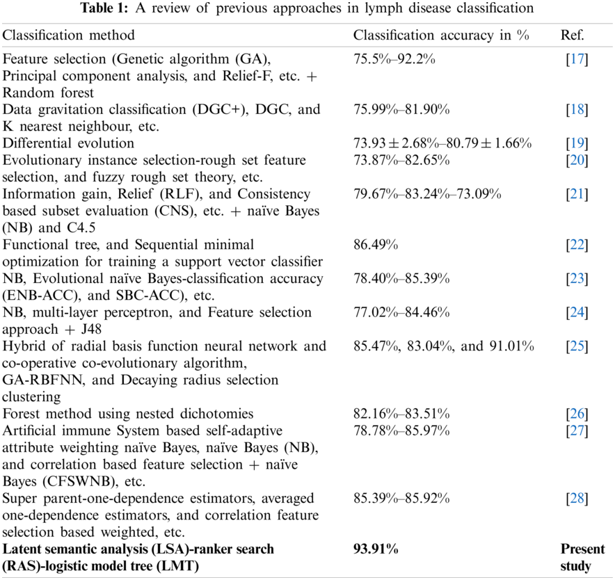
Classification approaches to machine learning have been implemented in the recognition of lymph disease in past studies [17–28]. Mainly, single classification methods [19,22], in combination with the feature selection approach [17,20,21,24], and combination with other classification methods [18,23,25,27,28] have been used in the analysis of the lymph disease dataset. Tab. 1 presents a short review of the classification approaches used in the analysis of the lymph disease dataset. Based on category wise analysis of the classification methods, it is obvious that the tree-based classification methods have been used mostly in the lymph disease recognition [17,22,28]. The maximum accuracy of 92.2% has been achieved using the selected features and random forest (RF) classifier [17]. The artificial neural network (ANN) classification methods implemented in some studies [24,25], like multi-layer perceptron (MLP) [24], and hybrids of radial basis function neural network and evolutionary algorithm [25]. The hybrid ANN method achieved improved recognition accuracy of 85.47% than MLP. The Bayesian classifiers [23,24] result in average recognition accuracy. Besides, in some recent studies, deep learning approaches have been implemented in disease diagnosis, like convolutional long short-term memory neural network in heartbeat classification [29], atrial fibrillation detection using adaptive residual network [30], and arrhythmia classification using fully connected neural networks [31], etc.
1.2 Motivation and Contribution of Present Study
It is obvious from the literature survey that the selected feature improves the recognition performance of the classification methods. The selection of an optimal set of features that can result in the maximum lymph disease recognition accuracy is still an existing challenge. With this motivation, an effective approach of feature generation (latent semantic analysis (LSA)) and selection (ranker search (RAS)) has been proposed which results in the maximum lymph disease recognition accuracy of classification methods. The main findings of the present study include the followings:
● An efficient approach of dimensionality reduction using the combination of feature generation and selection approaches.
● An effective recognition approach of lymph disease using the combination of an optimal subset of selected features.
● Comprehensive performance comparison of the proposed feature generation and selection method with other methods of attribute selection.
● Performance validation of the proposed approach using functions and tree-based classification methods.
● The maximum recognition accuracy of the classification methods using the feature subset selected with the proposed approach with methods in the reviewed literature.
Details of the lymph disease dataset are available in Section 2, Section 3 presents the proposed approach, analysis results are presented in Section 4, discussed in Section 5, and concluded in Section 6.
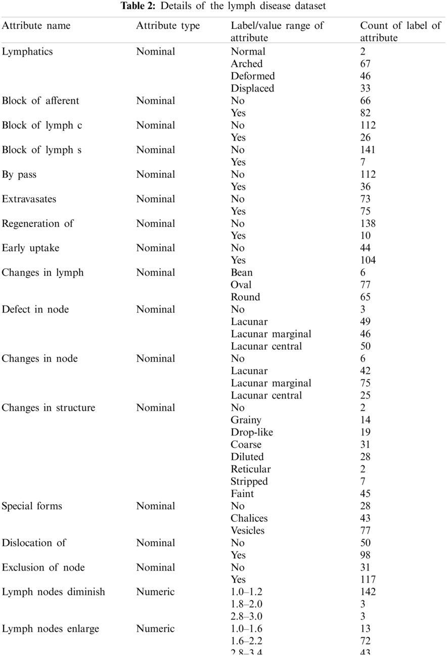
The lymphography dataset was accessed from the University of California Irvin's (UCI) machine learning repository [32]. A description of the lymphography dataset is available in Tab. 2. It contains two instances of normal cases and eighty-one, sixty-one, and four instances of metastases, malign lymph, and fibrosis cases of lymph disease, respectively. Fifteen nominal attributes (lymphatics, block of afferent, and block of lymph c, etc.) and three numerical attributes (lymph nodes diminish, lymph nodes enlarge, and number of nodes) of each of the instances have been observed without missing values.
3 Feature Generation, Selection, and Classification
The LSA method generates an effective set of features by combining the original attributes. The RAS selects an optimal subset of features from the LSA generated set. Subsequently, the selected optimal subset of features results in the improved recognition accuracy of MLP, simple linear logistic regression (SL), and sequential minimal optimization (SMO), functional tree (FT), and logistic model tree (LMT) classification methods. Fig. 1 presents a schematic diagram of the analysis and validation procedures. A PC (64-bit Windows 10, Intel(R) Core(TM) i5-4590 CPU@3.30 GHz, 8 GB RAM) was used in the implementation of attribute selection, feature generation and selection, classification methods, and their combination in WEKA [33]. A short description of attribute selection, feature generation, and selection, classification methods are as follows.
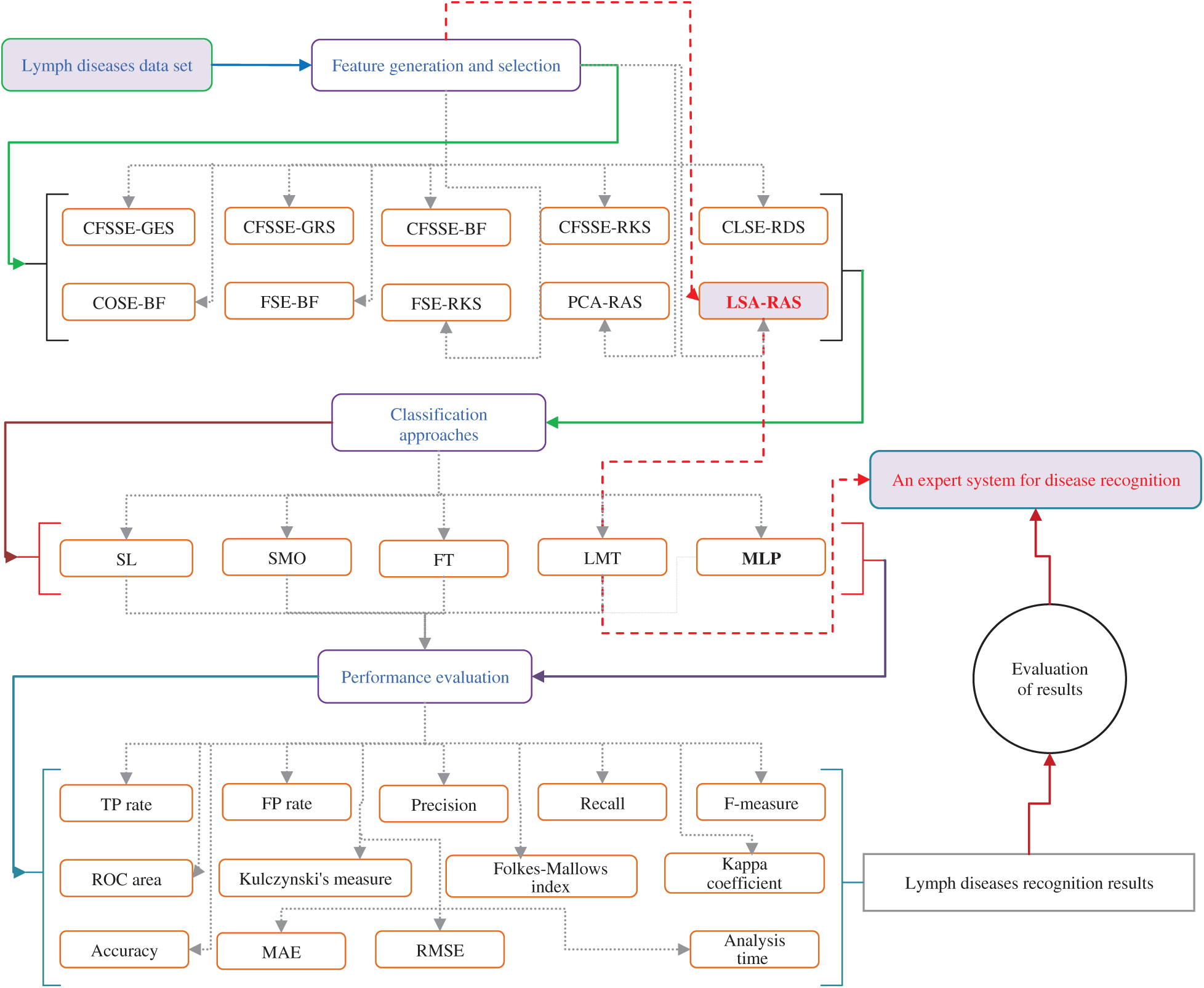
Figure 1: An overview of attribute selection, feature generation and selection, classification, and performance evaluation methods of the lymph disease
3.1 The Proposed LSA-RAS Approach of Feature Generation and Selection
The LSA measures the textual coherence of the nominal attributes. It is suitable for selecting an optimal subset of features, discarding the inappropriate features, and representation of instances in a novel semantic space for better discrimination, etc. [34]. The details of the LSA method are available in [34]. Firstly, the frequency (
3.2 Functions and Tree-Based Classification Approaches
Three functions-based classifiers (MLP, SL, and SMO) and two tree-based classifiers (FT, and LMT) have been implemented to test the efficiency of the LSA-RAS selected feature subset and other feature subsets in a 10-fold cross-validation.
It is a systematic arrangement of artificial neurons in different layers (input, hidden, and output). The input of a neuron is defined as
It implements regression function and boosting algorithm (LogitBoost) [37] in class recognition of an instance. The LogitBoost algorithm starts with the weight initialization as
SMO [36] is used in the training of the support vector machine (SVM) classifier. The decision function of binary SVM is defined as
FT [38] uses logistic regression functions at the inner nodes and/or leaves and a constructor function (generalized linear model (GLM)) to build the decision tree. GLM combines the original attributes to generate the novel attributes. Firstly, the constructor function is used to build the initial model. In the second step, the model is mapped to new attributes of dimension equal to the number of classes in the dataset. The new attributes represent the class belonging probability of an instance computed by using the constructor function. A merit function is used to evaluate the attribute with the original attributes. The FT was built using the following parameters: boosting iterations equal to 150, number of instances equal to 15 for the splitting of nodes, and
LMT is a combination of linear logistic regression (low variance high bias) and tree induction (high variance low bias) classification methods [39]. Logistic regression functions are generated at every node of the tree using the LogitBoost algorithm. An information gain criterion was used for the splitting of the tree, and after the complete formation of the tree, the CART algorithm was used for its pruning. The heuristic cross-validation was used to control the number of iterations of LogitBoost to avoid data overfitting. The additive logistic regression of the LogitBoost algorithm for each class
3.3 Additional Attributes and Feature Selection Methods
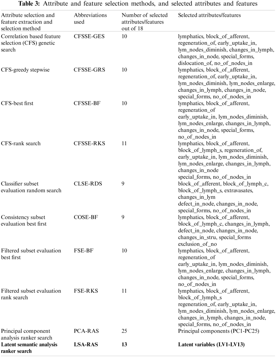
Nine feature selection methods (Tab. 3) have been used in the performance comparison analysis. The correlation-based feature selection genetic search (CFS-GES) method combines two approaches, correlation-based feature selection (CFS) and genetic search (GES). The CFS implements a correlation measure to select the feature which is highly correlated with the class and less correlated with the other features.
On the basis of the earlier correlation values, a merit measure
Redundant attributes are discarded using a threshold value of −1.80 [33]. A hill-climbing approach with a backtracking search approach was used in the selection of optimal attributes in the best first (BF) method. A forward search approach and search termination threshold value equal to 5 was used in the BF method in the present analysis [33]. BF method was used in combination with CFS, consistency subset evaluation, and filtered subset evaluation methods (Tab. 3). The rank search (RKS) approach uses a forward selection search method to generate an optimal subset of the attribute of maximum merit. The attributes are included one by one with the best attribute in each step to generate an optimal subset of attributes. Attribute evaluator (gain ratio with starting point equal to 0 and the step size equal to 1) was used to evaluate the attribute subset in each step after including an attribute until the merit of the attribute subset increases [21]. The RKS method was combined with the CFS and filtered subset evaluation (FSE) methods for the attribute ranking and selection (Tab. 3). Classifier subset evaluation (CLSE) implements a classification method in the selection of an optimal subset of attributes. The CLSE uses a ZeroR classification approach to compute the merit of the feature subset. For the numeric class, ZeroR predicts the mean of the numeric class and mode for the nominal class. This concept is used to compute the merit of an attribute subset in CLSE [33]. The random search (RDS) uses a random search approach to select an optimal subset of attributes. The RDS selects a random subset of attributes in finding the optimal subset. Another parameter used in the RDS method was a seed equal to 1 to generate a random number, and 25% of the search space [33]. The RDS was used in combination with the CLSE (Tab. 3). Consistency subset evaluation (COSE) selects an optimal subset of attributes on the basis of its level of consistency in class. The consistency
3.4 Performance Assessment Measures of Classification Approaches
Performance of classification approaches is evaluated on the basis of the average value of true positive (TP) rate, false positive (FP) rate, precision, recall, Kulczynski's measure (arithmetic mean of precision and recall), Folkes-Mallows index (geometrical mean of precision and recall), F-measure (harmonic mean of precision and recall), Kappa coefficient, receiver operating characteristic (ROC) area, and analysis time. The Kappa coefficient is computed using the number of instances in a row
4 Validation Results of the Proposed Approach and Comparative Analysis Results
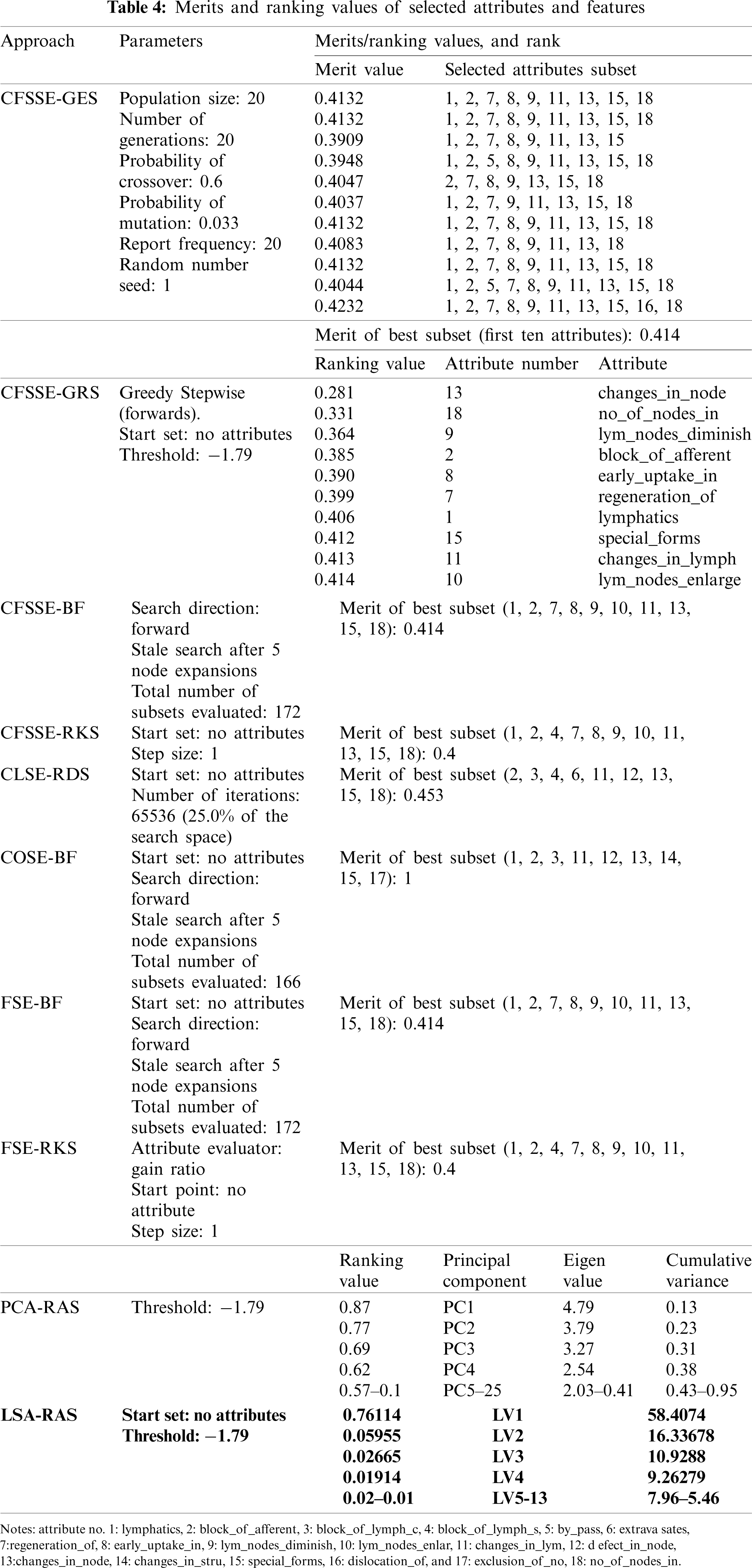
Tab. 3 summarizes the attributes and features selected by the different approaches. It is obvious that the CFSSE-RKS method selects a maximum number of attributes (11 out of 18) and PCA-RAS generates a maximum number of features. CFSSE-GES, CFSSE-GRS, and CFSSE-BF methods select a similar number of attributes (Tab. 3). The different attributes subsets are selected by the CFSSE-GES, and CFSSE-GRS methods, while the attribute subset selected by the CFSSE-GRS and CFSSE-BF is the same. It is also noticeable that the PCA-RAS and LSA-RAS methods select the optimal subset of features considering the contributions of all attributes, while the rest of the methods in Tab. 3 select an optimal subset of attributes. The parametric details of the attributes/feature selection methods and the merits/ranking of the selected subset of the attributes/features are summarized in Tab. 4. The performance of classification methods using selected subsets of attributes/features is summarized in Tab. 5. Tab. 6 presents the performance evaluation metrics of classification methods.
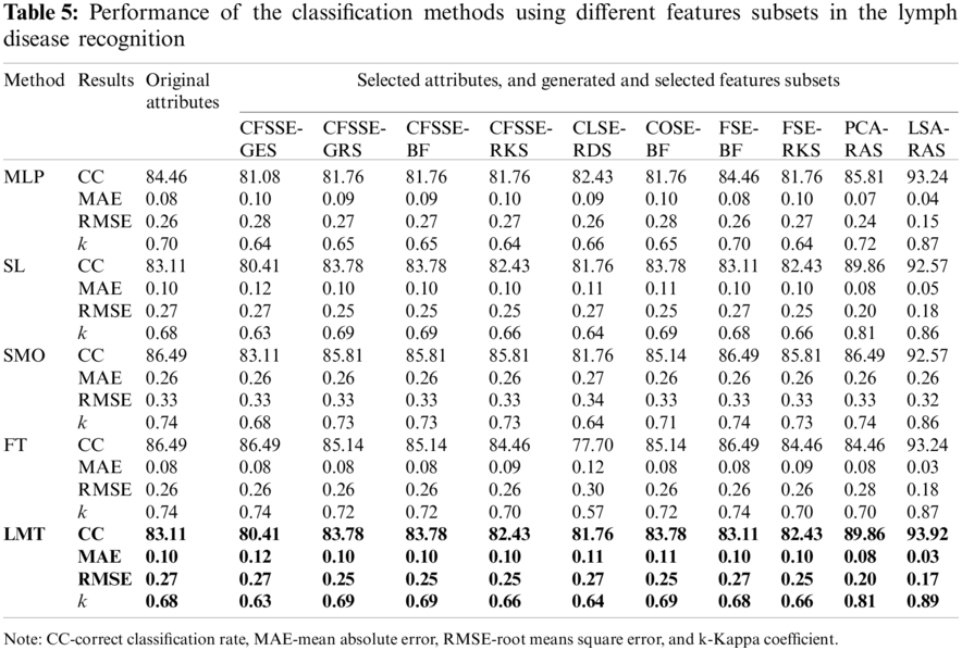
The LSA-RAS generated feature subset results in the maximum accuracy of classification methods (Tab. 5). Among the three functions-based classification methods, the maximum classification accuracy (93.24%) and the minimum value of mean absolute error (MAE) (0.04) have been achieved for the MLP. The LMT classifier achieved higher accuracy (93.92%) and the maximum value of the kappa coefficient (0.89) than the FT method.
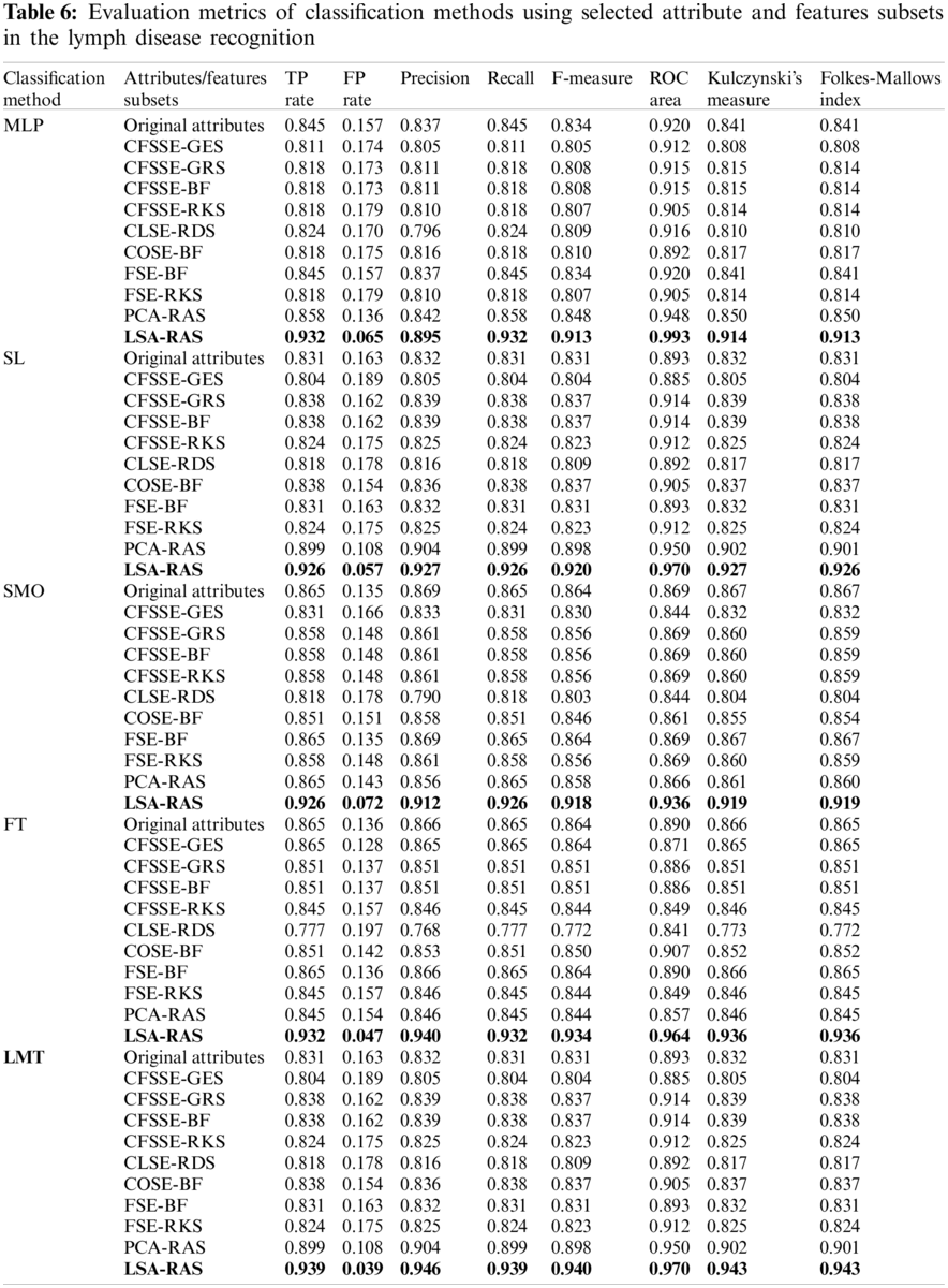
The LSA-RAS selected feature subset results in the improvement of 10.81% in the classification accuracy of the LMT classifier than the original attributes. Moreover, the accuracy of classification methods using most of the selected attribute subset except PCA-RAS and LSA-RAS selected feature subset is lower or comparable than using the original attributes. The LSA-RAS selected feature subset results in improved evaluation measures (maximum value of average the TP rate, Precision, Recall, F-measure, ROC area, Kulczynski's measure, and Folkes-Mallows index, and the minimum average value of FP rate) of each of the classification methods than other selected attribute subsets, selected feature subset, and original attributes. Furthermore, the LMT classification method using the LSA-RAS selected feature subset has the best values of earlier evaluation metrics than the rest of the classification method. A detailed class confusion matrix of each of the classification methods using the best performing LSA-RAS selected feature subset is summarized in Tab. 7. The MLP classification recognizes 138 out of 148 instances of lymph disease correctly. The maximum number of instances (80 out of 81) of metastases class is identified correctly (accuracy of 98.77%). Fig. 2 presents the error curve of the MLP method using three attribute subsets and one feature subset.
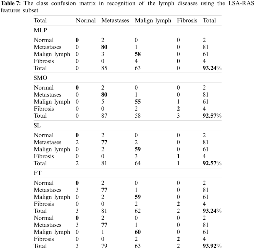
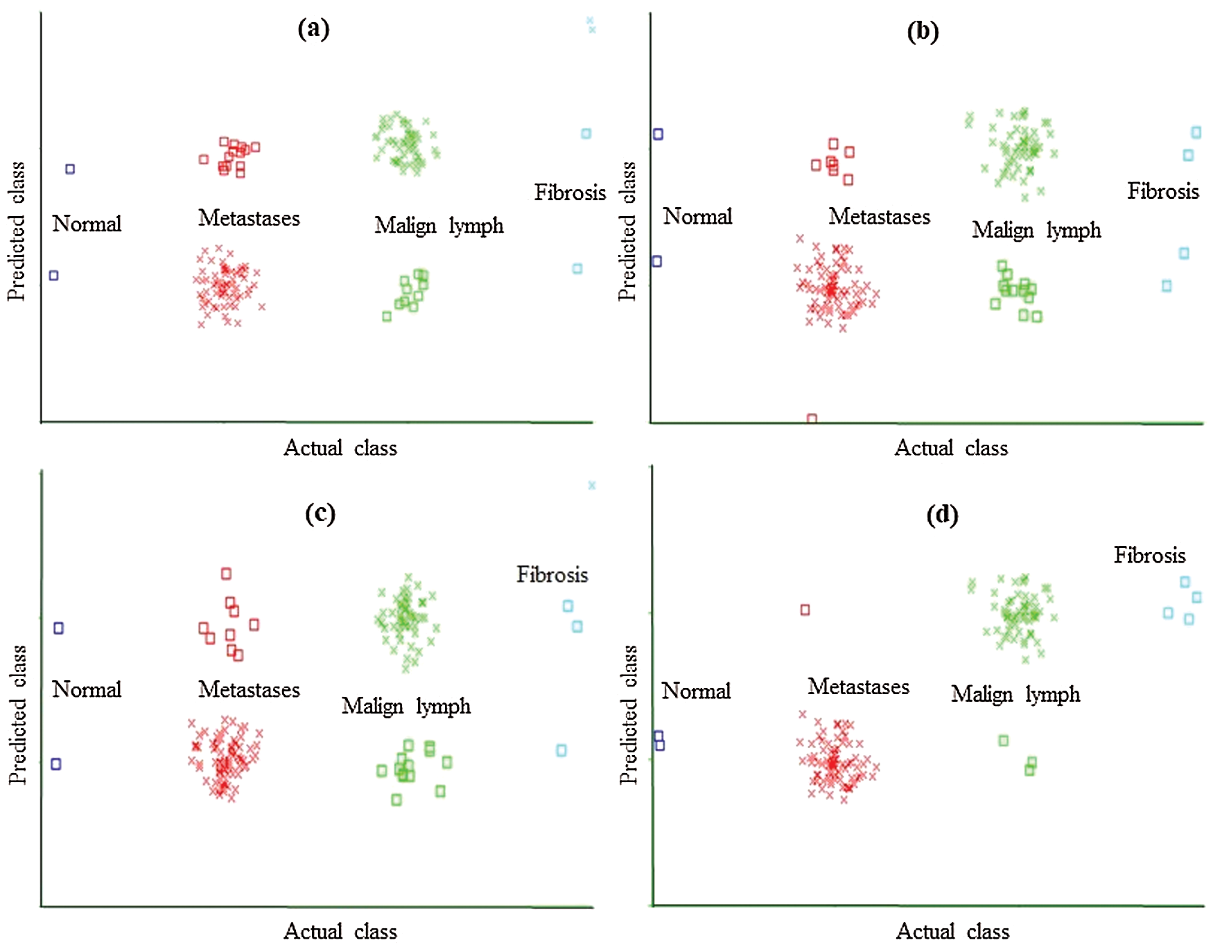
Figure 2: Classification error curve of MLP using (a) CFSSE-GES, (b) CLSE-RDS, (c) FSE-RKS, and (d) LSA-RAS selected attribute and feature subsets
The classification error in Fig. 2 is denoted by the square symbol. It is obvious that the LSA-RAS feature subset results in the minimum classification error (10) of MLP than rest three attribute subsets (Fig. 2d). It is analogous to the confusion matrix of MLP in Tab. 7. The CFSSE-GES selected attribute subset results in the maximum error of MLP (Fig. 2a). The error curve of the SL is presented in Fig. 3. The SL classification recognizes 137 out of 148 instances of lymph disease correctly. The maximum number of instances (59 out of 61) of malign lymph class is identified correctly (accuracy of 96.72%, Tab. 7). The LSA-RAS selected feature subset results in the minimum classification error (11) of the SL than rest three attribute subsets (Fig. 3d) which is similar to the confusion matrix of SL in Tab. 7. The maximum error of SL has been obtained for the CFSSE-GES selected attribute subset (Fig. 3a). Fig. 4 presents the error curve of the SMO classification method. Like SL, the SMO classification method also recognizes 137 out of 148 instances of lymph disease correctly though there is some difference in the confusion matrix (Tab. 7). The maximum number of instances (80 out of 81) of metastases class is identified correctly (accuracy of 98.77%, Tab. 7). The LSA-RAS selected feature subset results in the minimum classification error (11) of SMO than rest three attribute subsets (Fig. 4d) (analogous to the confusion matrix of SL in Tab. 7).
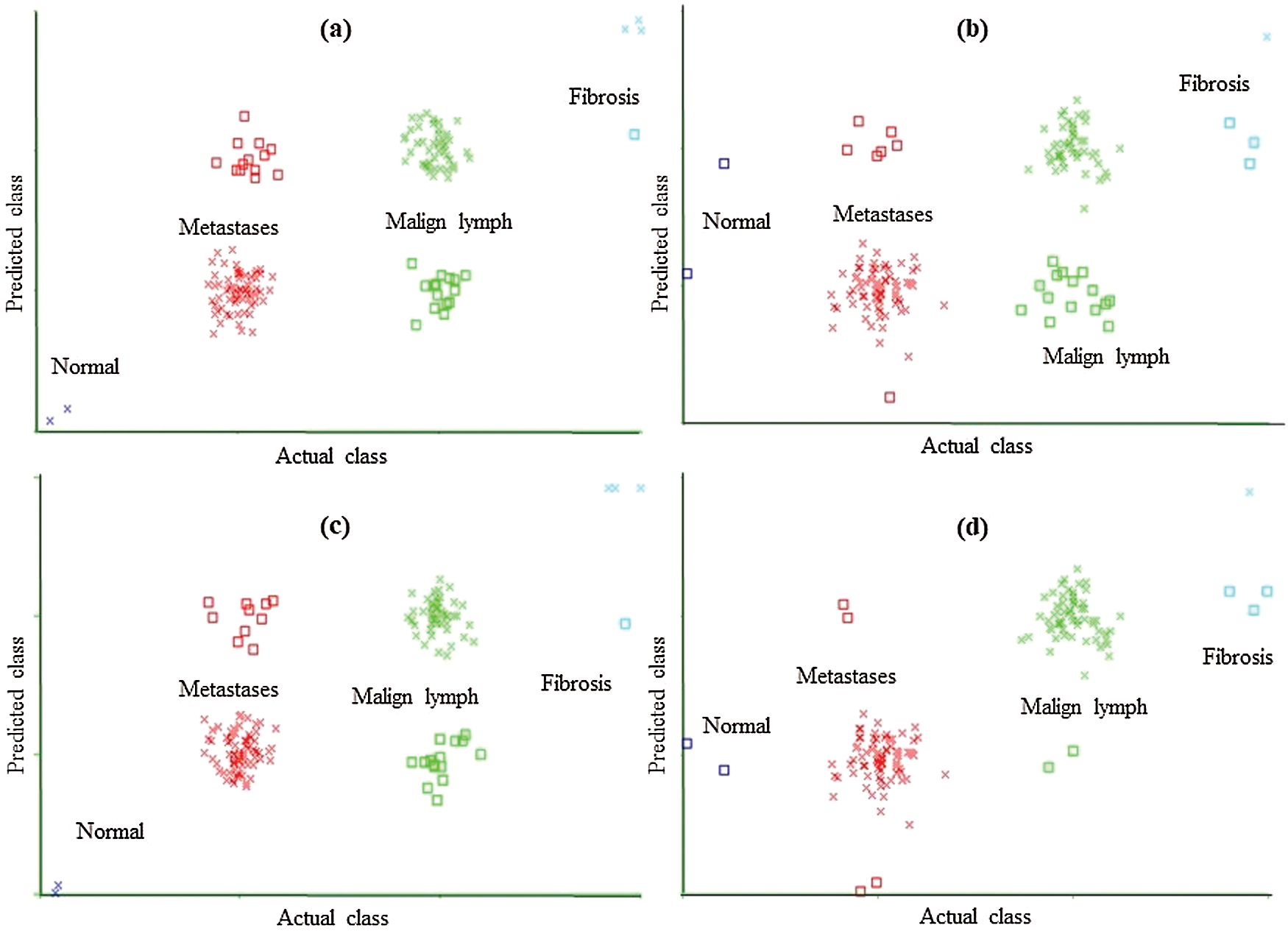
Figure 3: Classification error curve of SL using (a) CFSSE-GES, (b) CLSE-RDS, (c) FSE-RKS, and (d) LSA-RAS selected attribute and feature subsets
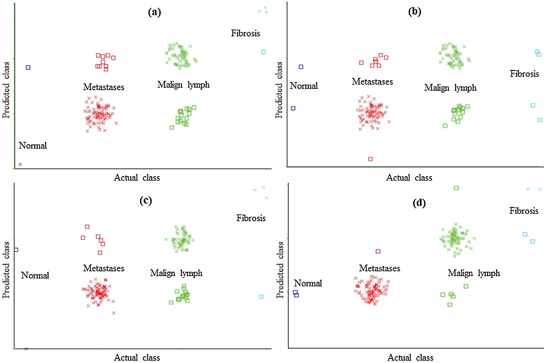
Figure 4: Classification error curve of SMO using (a) CFSSE-GES, (b) CLSE-RDS, (c) FSE-RKS, and (d) LSA-RAS selected attribute and feature subsets
The CLSE-RDS selected attribute subset results in the maximum error of the SMO (Fig. 4a). The error curve of the FT classification method using CFSSE-GES, CLSE-RDS, and FSE-RKS selected attribute subsets, and LSA-RAS selected feature subset is presented in Fig. 5. The FT classification method identifies 138 out of 148 instances of lymph disease correctly (confusion matrix in Tab. 7). The maximum number of instances (59 out of 61) of malign lymph class is identified correctly (accuracy of 96.72%). The LSA-RAS selected feature subset results in the minimum classification error (10) of the FT classifier than the rest three attributes subsets (Fig. 5d) (similar to the confusion matrix of FT in Tab. 7). CFSSE-GES and FSE-BF have the maximum and similar errors (Figs. 5a and 5c). Fig. 6 presents the error curve of the LMT classification method. The error curve in Fig. 6d represents that 139 out of 148 instances have been correctly identified by the LMT method using the LSA-RAS selected feature subset. It is analogous to the confusion matrix of the LMT method in Tab. 7. The maximum number of instances (60 out of 61) of malign lymph class is identified correctly (accuracy of 98.36%). The CFSSE-GES selected attribute subset results in the maximum error of the LMT (Fig. 6a). The LSA-RAS selected feature subset results in the improved value of the area under ROC of the classification methods than any other selected attribute subset, feature subset, and original attributes (Tab. 6). Furthermore, the maximum average area under the ROC was achieved for the LMT using the LSA-RAS selected feature subset.

Figure 5: Classification error curve of FT using (a) CFSSE-GES, (b) CLSE-RDS, (c) FSE-RKS, and (d) LSA-RAS selected attribute and feature subsets
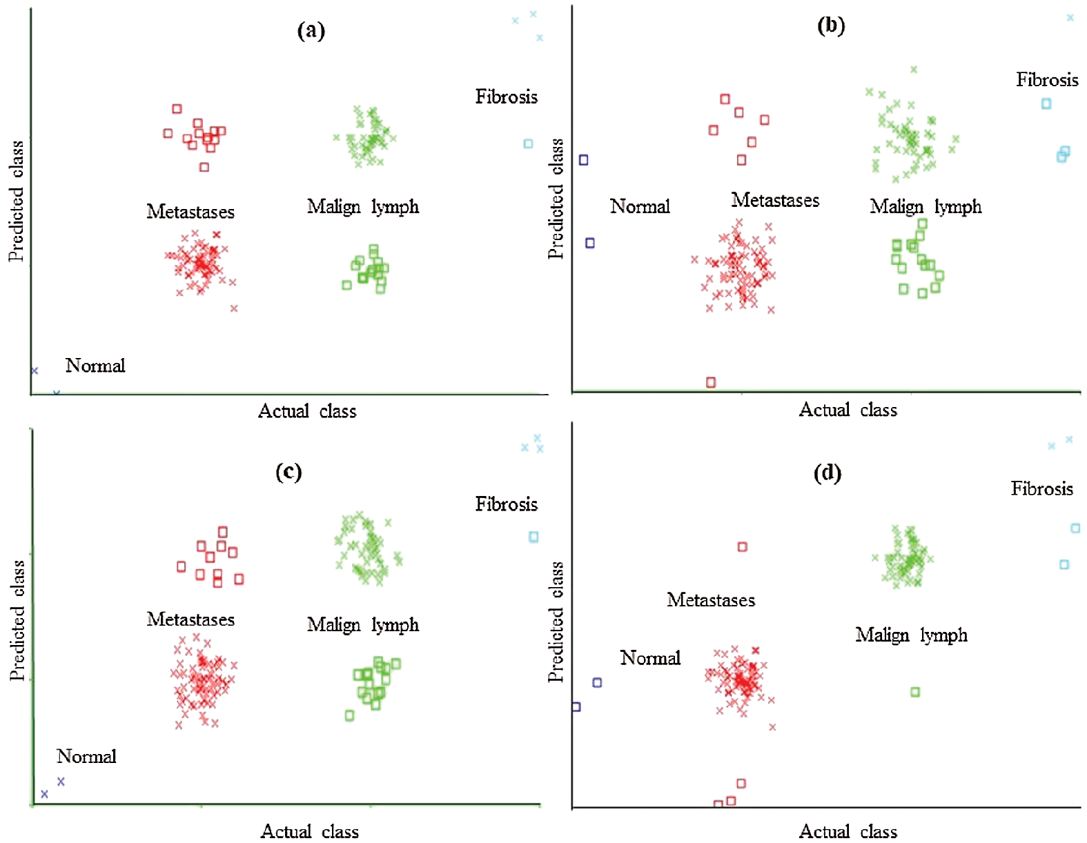
Figure 6: Classification error curve of LMT using (a) CFSSE-GES, (b) CLSE-RDS, (c) FSE-RKS, and (d) LSA-RAS selected attribute and feature subsets
The class-wise area under the ROC curve of LMT using the LSA-RAS selected feature subset is demonstrated in Fig. 7. It is obvious that the three positive classes (metastases, malign lymph class, fibrosis) of the lymph disease have an area under ROC ≥ 0.96. The minimum ROC area (0.43) was obtained for the normal class of the lymph disease while the fibrosis class of the lymph has the maximum ROC area (0.998). Fig. 8 represents the cost/benefit curve of LMT using the LSA-RAS selected feature subset of normal and three classes of lymph. The cost/benefit curve represents the error rate on the Y-axis and the probability of belonging to the positive class on the X-axis. The normal and fibrosis classes of lymph have higher error (100%, and 50%, respectively), consequently, the cost curve has a positive slope. The rest of the two classes metastases and malign have a lower error rate. The analysis time of each of the classification methods using the original attributes, selected attributes, and selected features are presented in Fig. 9. The MLP classification method has a maximum analysis time of 2.29 s using the FSE-BF selected attribute subset and the SMO method has a minimum analysis time of 0.01 s using the FSE RKS selected attribute subset. Moreover, the MLP has the maximum average analysis time of 0.793 s and the SMO has a minimum average analysis time of 0.037 s using original attributes and selected attributes, and selected features.
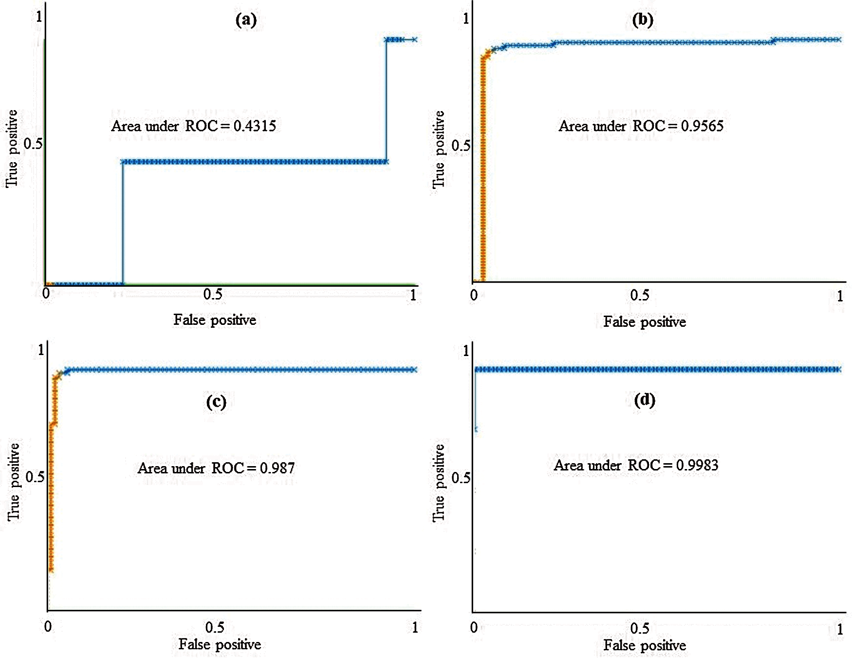
Figure 7: The area under the ROC curve of LMT using LSA-RAS selected feature subset for (a) normal, (b) metastases, (c) malign lymph, and (d) fibrosis classes of lymph diseases
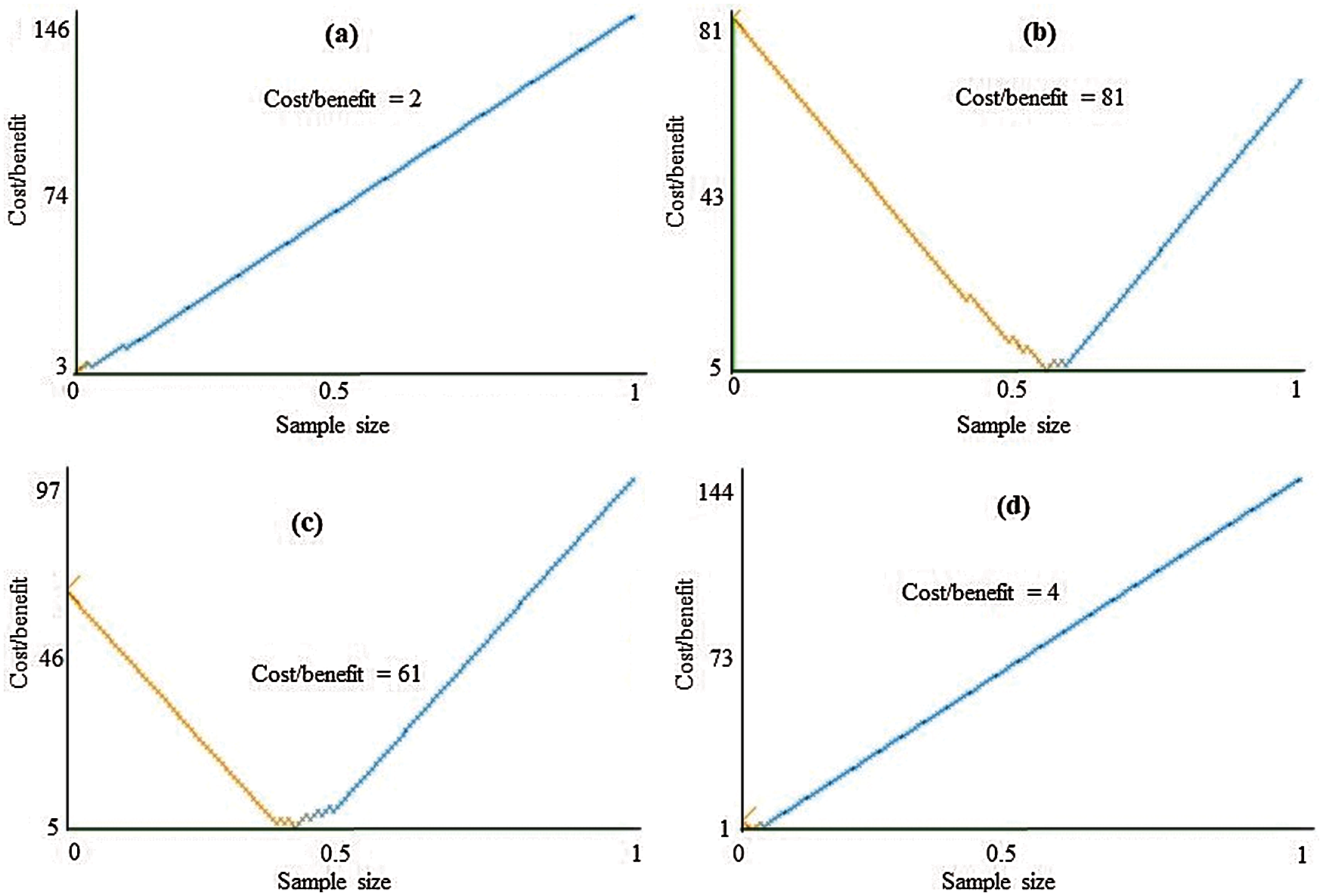
Figure 8: Cost/Benefit curve of LMT using LSA-RAS selected feature subset for (a) normal, (b) metastases, (c) malign lymph, and (d) fibrosis classes of lymph diseases
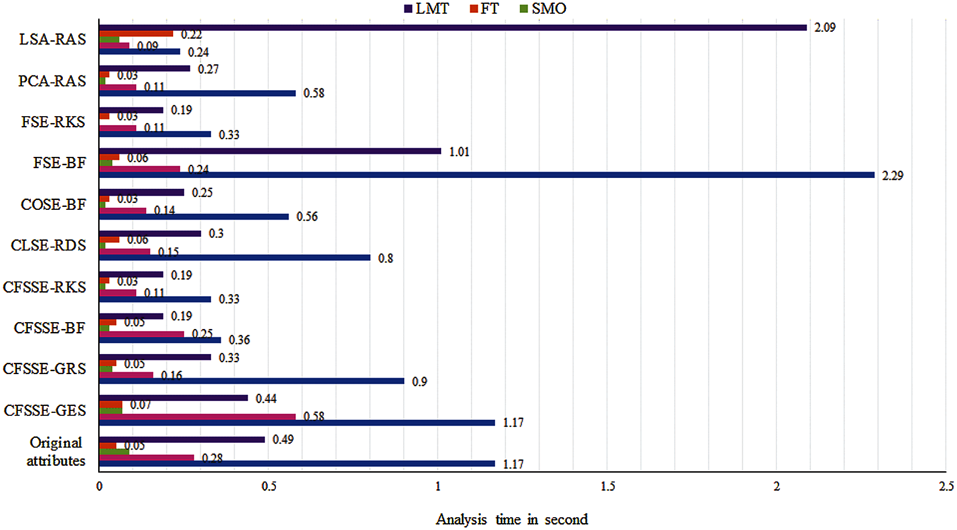
Figure 9: Analysis time of classification methods using original attributes and selected attributes, and selected and generated feature subsets
5 Discussions of Validation and Comparative Analysis Results
The PCA-RAS and LSA-RAS methods consider the contribution of all attributes in the generation and selection of an optimal subset of novel features. This is the reason for the better performance of classification methods in lymph disease recognition using the PCA-RAS and LSA-RAS selected feature subset than the original attributes and other selected subset of attributes. Though the better performance of the LSA-RAS selected feature than the PCA-RAS selected feature, in-class recognition is due to the majority of the nominal attribute (15 out of 18) in the lymph disease dataset.
The PCA minimizes the correlation and maximizes the variance of the three original numerical attributes, while the LSA measures the textual coherence of most of the nominal attributes effectively and generates novel latent variables that result in a significant improvement in the accuracy of classification methods. The deprived performances of the eight attribute selection methods (Tab. 3) in class recognition of the lymph diseases are due to the selection of a few significant attributes of the original data. It may cause the loss of the class identity information on the discarded attributes and hence the substandard recognition performance of the classification methods using the selected attributes than the original attribute, and the PCA-RAS and LSA-RAS selected feature subsets. Analysis results in Figs. 2–8 and Tabs. 2–7 confirm the better performance of the tree-based than the function-based classification methods using the LSA-RAS selected feature subset. Specifically, the LMT achieved the best recognition accuracy than the rest of the classification methods and the performance of the FT is comparable to MLP and better than the SL and SMO methods. Using the efficient LSA-RAS selected feature subset is the reason for the improved recognition accuracy of each of the classification methods. The improved performance of classification methods in recognition of lymph disease in combination with the feature selection methods is also discussed in some past studies summarized in Tab. 1, like the performance improvement of RF using GA, PCA, and ReliefF, etc. (maximum accuracy of 92.2% using GA selected feature subset) [17]; the maximum accuracy of 82.65% of classification method using the rough set selected feature subset [20]; improved accuracy of NB and C4.5 classification methods using information gain (IG), relief, and consistency-based subset evaluation (CNS), etc. (maximum accuracy of 83.24%) [21]; improved accuracy of NB, MLP, and J48 classification method using the IG, gain ratio, and symmetrical, etc. (maximum accuracy of 84.46%) [24]; and improved accuracy (84.94 ± 8.42%) of the NB method using the artificial immune system self-adaptive attribute weighting method [27], etc.
The LSA or the combination of the LSA with RAS in lymph disease recognition is not implemented before in the previously published research. Though, the LSA method has been implemented in different applications [41–45], including topic modeling [41], remote sensing image fusion [42], patient-physician communication [43], essay evaluation [44], and psychosis prediction [45], etc. The semantic information is obtained by combining the likelihood of the co-occurrence in the LSA. Also, the latent variables attempt to link the nominal attributes of the instance to their respective class maximally, which causes the improved performance of the classification methods. The improved performance of the RAS method in feature selection is due to its characteristics to combine the entropy, gain-ratio, and relief criteria. The combination of the earlier three criteria reduces the redundancy in the selected feature subset. Some of them have been used independently in the feature selection of the lymph dataset [17,21,24], like reliefF (accuracy of 84.2%) [17], information gain, and reliefF (accuracy of 82.63%, and 81.47%) [21], and information gain, gain ratio, and reliefF (accuracy of 77.02%–80.40%) [24], etc. Among the three functions-based classification methods, the MLP results in the maximum accuracy, using the LSA-RAS selected feature subset. The tree-based LMT achieved the maximum recognition accuracy, using a similar feature subset. The best accuracy of the tree-based classification method and improved accuracy of the function-based classification method is also confirmed in the earlier studies [17,22,24–26], like the best recognition accuracy of 92.2% of random forest method [17], maximum accuracy of 86.49% of SMO and FT methods using the original attributes of lymph dataset [22], the accuracy of 84.46% of MLP, using chi-square selected and original attributes [24], the training accuracy of 85.47% of hybrid radial basis function neural network [25], and the maximum accuracy of 83.51% of ensembles of decision trees [26], etc.
The better performance of the tree-based classification methods; LMT and FT are due to the less number of adjustable parameters after using a significant subset of features selected by the LSA-RAS method, a reduced amount of noise of original attributes in latent variables, and negligible influence of noise, etc. The improved performance of the MLP method is due to the reduced uncertainty of the input and output by using the LSA-RAS selected feature subset. Among the implemented feature selection methods in the recognition of the lymph disease in the previous study [17,20,21,24,27], the best accuracy has been achieved for the combination of the GA and random forest classification methods [17]. The proposed approach LSA-RAS-LMT in the present study achieved the maximum recognition accuracy of the lymph disease than previously published reports. A significant improvement in the accuracy of the LMT (10.81%), SL (9.46), and ML (8.78%) has been achieved (Tab. 5). The analysis time of the LSA-RAS-LMT approach in the present analysis of the lymph dataset was 2.09 s (Fig. 9). It is in between the analysis time 0.02 s–11.77 s of [20] and, 0.0004 s–0.0051 s (Linux cluster node (Inter(R) Xeon(R) @3.33 GHz, and 3 GB memory) [28]. The area under the ROC of the LSA-RAS-LMT approach in the present analysis is equal to 0.97 (Tab. 6). It is higher than the area under ROC of other approaches [17,19,23,27], like 0.843-0.954 [17], 80.48 [19], 91.3757 ± 3.25–91.8005 ± 3.61 [23], and 92.99 ± 4.15–95.01 ± 4.87 [27]. The LSA-RAS-LMT method has the maximum value of the kappa coefficient (0.89) (Tab. 5) in the present analysis. It is also higher than the earlier achieved value of the kappa coefficient [17,18], like 0.512–0.879 [17] and 0.500–0.629 [18].
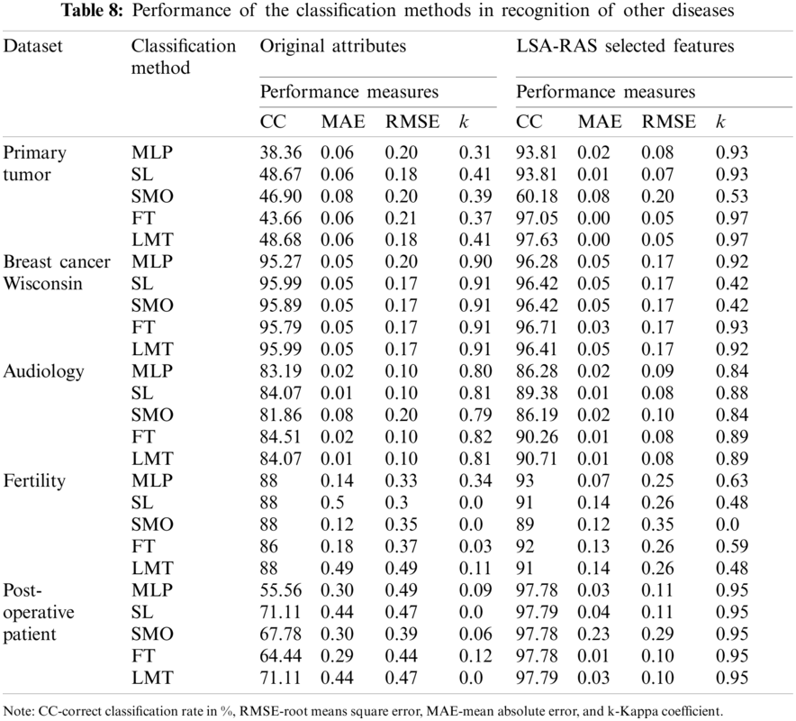
Moreover, the LSA-RAS approach has been validated in the recognition of other benchmark diseases (primary tumor, breast cancer, audiology, fertility, and post-operative patient) [32]. The performance of classification approaches is summarized in Tab. 8. It is obvious that the LSA-selected features subset results in improved accuracy of each of the classification methods than the original attributes. Specifically, a major improvement in accuracy of MLP in the primary tumor (55.45%), SL and SMO in the post-operative patient (26.61%), and FT (53.39%) and LMT (48.95%) in primary tumor has been noticed. The LMT classifier has an improved recognition performance in the analysis of most of the disease datasets.
Deep neural networks such as convolutional and recurrent neural networks are used mainly in the preprocessing and classification of the image, text, and continuous data successfully in the past studies [11–12,29–31]. Though the lymph and other disease datasets selected in the present study contains the discrete values of numeric and nominal attributes, therefore, the direct implementation of the deep neural networks and its comparison with the proposed approach is not feasible. However, there is a need to explore the possibility in the future research.
6 Conclusions and Research Scope
In the present study, a competent feature generation and selection method (LSA-RAS) of lymph disease recognition has been implemented and validated. The LSA-RAS method results in the improved accuracy of different classification methods. The tree-based methods achieved better performance than the function-based classification methods using the LSA-RAS selected feature subset. Furthermore, hybrids approach (LSA-RAS-LMT) using the combination of feature generation and selection, and classification methods achieved the maximum recognition accuracy and improved the value of other evaluation metrics than other approaches available in the published literature. The LSA-RAS-LMT approach is efficient in the recognition of the lymph disease and analogous disease datasets. Future research will focus on further improvement in the accuracy of the classification methods for lymph disease recognition.
Acknowledgement: This work is supported by the Startup Foundation for Introducing Talent of NUIST. The authors acknowledge the anonymous reviewers for their valued comments and suggestions.
Funding Statement: This work is supported by the Startup Foundation for Introducing Talent of NUIST, Project No. 2243141701103.
Conflicts of Interest: The authors declare that they have no conflicts of interest to report regarding the present study.
1. Yassin, N. I., Omran, S., El Houby, E. M., Allam, H. (2018). Machine learning techniques for breast cancer computser aided diagnosis using different image modalities: A systematic review. Computer Methods and Programs in Biomedicine, 156, 25–45. DOI 10.1016/j.cmpb.2017.12.012. [Google Scholar] [CrossRef]
2. Chan, H. P., Hadjiiski, L. M., Samala, R. K. (2020). Computer-aided diagnosis in the era of deep learning. Medical Physics, 47(5), e218–e227. DOI 10.1002/mp.13764. [Google Scholar] [CrossRef]
3. Roth, H. R., Lu, L., Liu, J., Yao, J., Seff, A. et al. (2016). Improving computer-aided detection using convolutional neural networks and random view aggregation. IEEE Transactions on Medical Imaging, 35(5), 1170–1181. DOI 10.1109/TMI.2015.2482920. [Google Scholar] [CrossRef]
4. Moore Jr, J. E., Bertram, C. D. (2018). Lymphatic system flows. Annual Review of Fluid Mechanics, 50, 459–482. DOI 10.1146/annurev-fluid-122316-045259. [Google Scholar] [CrossRef]
5. Suami, H. (2017). Lymphosome concept: Anatomical study of the lymphatic system. Journal of Surgical Oncology, 115(1), 13–17. DOI 10.1002/jso.24332. [Google Scholar] [CrossRef]
6. Leone, A., Diorio, G. J., Pettaway, C., Master, V., Spiess, P. E. (2017). Contemporary management of patients with penile cancer and lymph node metastasis. Nature Reviews Urology, 14(6), 335–347. DOI 10.1038/nrurol.2017.47. [Google Scholar] [CrossRef]
7. Hu, D., Li, L., Li, S., Wu, M., Ge, N. et al. (2019). Lymphatic system identification, pathophysiology and therapy in the cardiovascular diseases. Journal of Molecular and Cellular Cardiology, 133, 99–111. DOI 10.1016/j.yjmcc.2019.06.002. [Google Scholar] [CrossRef]
8. Arrivé, L., Monnier-Cholley, L., Cazzagon, N., Wendum, D., Chambenois, E. et al. (2019). Non-contrast MR lymphography of the lymphatic system of the liver. European Radiology, 29(11), 5879–5888. DOI 10.1007/s00330-019-06151-6. [Google Scholar] [CrossRef]
9. Masoudi, M., Pourreza, H. R., Saadatmand-Tarzjan, M., Eftekhari, N., Zargar, F. S. et al. (2018). A new dataset of computed-tomography angiography images for computer-aided detection of pulmonary embolism. Scientific Data, 5(1), 1–9. DOI 10.1038/sdata.2018.180. [Google Scholar] [CrossRef]
10. Wang, H., Zhou, Z., Li, Y., Chen, Z., Lu, P. et al. (2017). Comparison of machine learning methods for classifying mediastinal lymph node metastasis of non-small cell lung cancer from 18 F-fDG PET/CT images. EJNMMI Research, 7(1), 1–11. DOI 10.1186/s13550-017-0260-9. [Google Scholar] [CrossRef]
11. Shin, H. C., Roth, H. R., Gao, M., Lu, L., Xu, Z. et al. (2016). Deep convolutional neural networks for computer-aided detection: CNN architectures, dataset characteristics and transfer learning. IEEE Transactions on Medical Imaging, 35(5), 1285–1298. DOI 10.1109/TMI.42. [Google Scholar] [CrossRef]
12. Faust, O., Hagiwara, Y., Hong, T. J., Lih, O. S., Acharya, U. R. (2018). Deep learning for healthcare applications based on physiological signals: A review. Computer Methods and Programs in Biomedicine, 161, 1–13. DOI 10.1016/j.cmpb.2018.04.005. [Google Scholar] [CrossRef]
13. Jain, D., Singh, V. (2018). Feature selection and classification systems for chronic disease prediction: A review. Egyptian Informatics Journal, 19(3), 179–189. DOI 10.1016/j.eij.2018.03.002. [Google Scholar] [CrossRef]
14. Rahman, M., Usman, O. L., Muniyandi, R. C., Sahran, S., Mohamed, S. et al. (2020). A review of machine learning methods of feature selection and classification for autism spectrum disorder. Brain Sciences, 10(12), 949–972. DOI 10.3390/brainsci10120949. [Google Scholar] [CrossRef]
15. Cilia, N. D., De Stefano, C., Fontanella, F., Raimondo, S., Scotto di Freca, A. (2019). An experimental comparison of feature-selection and classification methods for microarray datasets. Information, 10(3), 109–122. DOI 10.3390/info10030109. [Google Scholar] [CrossRef]
16. Agor, J., Özaltın, O. Y. (2019). Feature selection for classification models via bilevel optimization. Computers & Operations Research, 106, 156–168. DOI 10.1016/j.cor.2018.05.005. [Google Scholar] [CrossRef]
17. Azar, A. T., Elshazly, H. I., Hassanien, A. E., Elkorany, A. M. (2014). A random forest classifier for lymph diseases. Computer Methods and Programs in Biomedicine, 113(2), 465–473. DOI 10.1016/j.cmpb.2013.11.004. [Google Scholar] [CrossRef]
18. Cano, A., Zafra, A., Ventura, S. (2013). Weighted data gravitation classification for standard and imbalanced data. IEEE Transactions on Cybernetics, 43(6), 1672–1687. DOI 10.1109/TSMCB.2012.2227470. [Google Scholar] [CrossRef]
19. de Falco, I. (2013). Differential evolution for automatic rule extraction from medical databases. Applied Soft Computing, 13(2), 1265–1283. DOI 10.1016/j.asoc.2012.10.022. [Google Scholar] [CrossRef]
20. Derrac, J., Cornelis, C., García, S., Herrera, F. (2012). Enhancing evolutionary instance selection algorithms by means of fuzzy rough set based feature selection. Information Sciences, 186(1), 73–92. DOI 10.1016/j.ins.2011.09.027. [Google Scholar] [CrossRef]
21. Hall, M. A., Holmes, G. (2003). Benchmarking attribute selection techniques for discrete class data mining. IEEE Transactions on Knowledge and Data Engineering, 15(6), 1437–1447. DOI 10.1109/TKDE.2003.1245283. [Google Scholar] [CrossRef]
22. Jha, S. K., Pan, Z., Elahi, E., Patel, N. (2019). A comprehensive search for expert classification methods in disease diagnosis and prediction. Expert Systems, 36(1), e12343. DOI 10.1111/exsy.12343. [Google Scholar] [CrossRef]
23. Jiang, L., Cai, Z., Zhang, H., Wang, D. (2012). Not so greedy: Randomly selected naive Bayes. Expert Systems with Applications, 39(12), 11022–11028. DOI 10.1016/j.eswa.2012.03.022. [Google Scholar] [CrossRef]
24. Karabulut, E. M., Özel, S. A., Ibrikci, T. (2012). A comparative study on the effect of feature selection on classification accuracy. Procedia Technology, 1, 323–327. DOI 10.1016/j.protcy.2012.02.068. [Google Scholar] [CrossRef]
25. Li, M., Tian, J., Chen, F. (2008). Improving multiclass pattern recognition with a co-evolutionary RBFNN. Pattern Recognition Letters, 29(4), 392–406. DOI 10.1016/j.patrec.2007.10.019. [Google Scholar] [CrossRef]
26. Rodríguez, J. J., García-Osorio, C., Maudes, J. (2010). Forests of nested dichotomies. Pattern Recognition Letters, 31(2), 125–132. DOI 10.1016/j.patrec.2009.09.015. [Google Scholar] [CrossRef]
27. Wu, J., Pan, S., Zhu, X., Cai, Z., Zhang, P. et al. (2015). Self-adaptive attribute weighting for naive Bayes classification. Expert Systems with Applications, 42(3), 1487–1502. DOI 10.1016/j.eswa.2014.09.019. [Google Scholar] [CrossRef]
28. Wu, J., Pan, S., Zhu, X., Zhang, P., Zhang, C. (2016). Sode: Self-adaptive one-dependence estimators for classification. Pattern Recognition, 51, 358–377. DOI 10.1016/j.patcog.2015.08.023. [Google Scholar] [CrossRef]
29. Wang, H., Shi, H., Lin, K., Qin, C., Zhao, L. et al. (2020). A high-precision arrhythmia classification method based on dual fully connected neural network. Biomedical Signal Processing and Control, 58, 101874. DOI 10.1016/j.bspc.2020.101874. [Google Scholar] [CrossRef]
30. Jin, Y., Qin, C., Liu, J., Lin, K., Shi, H. et al. (2020). A novel domain adaptive residual network for automatic atrial fibrillation detection. Knowledge-Based Systems, 203, 106122. DOI 10.1016/j.knosys.2020.106122. [Google Scholar] [CrossRef]
31. Jin, Y., Qin, C., Liu, J., Li, Z., Shi, H. et al. (2021). A novel incremental and interactive method for actual heartbeat classification with limited additional labeled samples. IEEE Transactions on Instrumentation and Measurement, 70, 1–12. DOI 10.1109/TIM.2021.3069021. [Google Scholar] [CrossRef]
32. Dua, D., Graff, C. (2019). UCI Machine learning repository. Irvine, CA: University of California, School of Information and Computer Science. http://archive.ics.uci.edu/ml. [Google Scholar]
33. Frank, E., Hall, M. A., Witten, I. H. (2016). The WEKA Workbench. Online Appendix for “Data Mining: Practical Machine Learning Tools and Techniques”, pp. 1–128. USA: Morgan Kaufmann. [Google Scholar]
34. Dumais, S. T. (2004). Latent semantic analysis. Annual Review of Information Science and Technology, 38(1), 188–230. DOI 10.1002/aris.1440380105. [Google Scholar] [CrossRef]
35. Liu, H., Motoda, H. (2012). Feature selection for knowledge discovery and data mining. USA: Springer. [Google Scholar]
36. Christopher, M. B. (2016). Pattern recognition and machine learning. USA: Springer. [Google Scholar]
37. Kotsiantis, S. B. (2005). Logitboost of simple Bayesian classifier. Informatica, 29(1), 53–59. http://www.informatica.si/index.php/informatica/article/viewFile/17/11. [Google Scholar]
38. Gama, J. (2004). Functional trees. Machine Learning, 55(3), 219–250. DOI 10.1023/B:MACH.0000027782.67192.13. [Google Scholar] [CrossRef]
39. Landwehr, N., Hall, M., Frank, E. (2005). Logistic model trees. Machine Learning, 59(1–2), 161–205. DOI 10.1007/s10994-005-0466-3. [Google Scholar] [CrossRef]
40. Ben-David, A. (2008). Comparison of classification accuracy using cohen's weighted kappa. Expert Systems with Applications, 34(2), 825–832. DOI 10.1016/j.eswa.2006.10.022. [Google Scholar] [CrossRef]
41. Kim, S., Park, H., Lee, J. (2020). Word2vec-based latent semantic analysis (W2V-lSA) for topic modeling: A study on blockchain technology trend analysis. Expert Systems with Applications, 152, 113401. DOI 10.1016/j.eswa.2020.113401. [Google Scholar] [CrossRef]
42. Fernandez-Beltran, R., Haut, J. M., Paoletti, M. E., Plaza, J., Plaza, A. et al. (2018). Remote sensing image fusion using hierarchical multimodal probabilistic latent semantic analysis. IEEE Journal of Selected Topics in Applied Earth Observations and Remote Sensing, 11(12), 4982–4993. DOI 10.1109/JSTARS.4609443. [Google Scholar] [CrossRef]
43. Vrana, S. R., Vrana, D. T., Penner, L. A., Eggly, S., Slatcher, R. B. et al. (2018). Latent semantic analysis: A new measure of patient-physician communication. Social Science & Medicine, 198, 22–26. DOI 10.1016/j.socscimed.2017.12.021. [Google Scholar] [CrossRef]
44. Zupanc, K., Bosnić, Z. (2017). Automated essay evaluation with semantic analysis. Knowledge-Based Systems, 120, 118–132. DOI 10.1016/j.knosys.2017.01.006. [Google Scholar] [CrossRef]
45. Rezaii, N., Walker, E., Wolff, P. (2019). A machine learning approach to predicting psychosis using semantic density and latent content analysis. NPJ Schizophrenia, 5(1), 1–12. DOI 10.1038/s41537-019-0077-9. [Google Scholar] [CrossRef]
 | This work is licensed under a Creative Commons Attribution 4.0 International License, which permits unrestricted use, distribution, and reproduction in any medium, provided the original work is properly cited. |