| Computer Modeling in Engineering & Sciences |
DOI: 10.32604/cmes.2021.017704
ARTICLE
An XBi-CFAO Method for the Optimization of Multi-Layered Variable Stiffness Composites Using Isogeometric Analysis
1School of Mechanical Science and Engineering, Huazhong University of Science & Technology, Wuhan, 430074, China
2School of Mechanical Engineering, Yangtze University, Jingzhou, 434023, China
*Corresponding Author: Qifu Wang. Email: wangqf@hust.edu.cn
Received: 31 May 2021; Accepted: 27 July 2021
Abstract: This paper presents an effective fiber angle optimization method for two and multi-layered variable stiffness composites. A gradient-based fiber angle optimization method is developed based on isogeometric analysis (IGA). Firstly, the element densities and fiber angles for two and multi-layered composites are synchronously optimized using an extended Bi-layered continuous fiber angle optimization method (XBi-CFAO). The densities and fiber angles in the base layer are attached to the control points. The structure response and sensitivity analysis are accomplished using the non-uniform rational B-spline (NURBS) based IGA. By the benefit of the B-spline space, this method is free from checkerboards, and no additional filtering is needed to smooth the sensitivity numbers. Then the curved fiber paths are generated using the streamline method and the discontinuous fiber paths are smoothed using a partitioned selection process. The proposed method in the paper can alleviate the phenomenon of fiber discontinuity, enhance information retention for the optimized fiber angles of the singular points and save calculating resources effectively.
Keywords: Isogeometric analysis; fiber angle optimization; variable stiffness laminates; fiber path optimization; topology optimization
The last two decades have witnessed the tremendous progress of advanced fiber reinforced plastics (FRP) and the increasingly usage of FRP in the aerospace and automotive industries [1–4]. Benefit from the rapid development of automated fiber placement (AFP) technologies [5–7] the variable stiffness laminates (VSLs) emerged [1–3,8–11]. These VSLs are reinforced by continuous fibers with curved trajectories within each layer, and so that they provide the engineers full potential and design flexibility by substantially enlarging the design space when compared with traditional constant stiffness laminates.
To exploit the potential and design freedom enabled by VSLs, a variety of design and optimization methods are actively developed [11]. Such as the discrete material optimization (DMO) [12–14], bi-value coding parameterization method (BCP) [15,16], and continuous fiber angle optimization method (CFAO) [17–20].
However, the design and optimization of VSLs with curvilinear fibers are still challenging. Because of the processing characteristics of curved fiber variable stiffness composites, how to improve the properties of composites while satisfying the manufacturing constraints has become an urgent problem to be solved [14,17,21].
In practice, the FEM method is utilized for structure response analysis in topology optimization. But there are some drawbacks if the conventional FEM method is used, e.g., the low continuity between the elements, and the low efficiency for high-order elements. In recent years, IGA proposed by Hughes et al. [22] has been widely used for the optimization of variable-stiffness panels [3,8,23,24]. As a novel and promising numerical method for structural analysis, IGA shows advantage in accurate representation of geometric models for structures with complex geometry [25–27]. The same basis functions are employed for geometry description and the structure response field variables representation as well, in the IGA method. Due to its high accuracy and high continuity, IGA is widely used in topology optimization [25,28,29] and fiber angle optimization problems [3,8,23,24,30]. As mentioned in [23], IGA is particularly suitable for the optimization of variable-stiffness composites benefits from the local support property of the NURBS basis function. The curved fiber paths of the VSLs are continuously laying in most of areas. In the CFAO method, the fiber angles are set as design variables during the optimization process. The control points-based-IGA can optimize the design variables attached to the control points, such as densities and fiber angles. The element parameters profit from the local support characteristics of the B-spline space, and they are naturally filtered. It should be pointed out that the natural filtering technique from the local support characters is naturally used in the NURBS-based-IGA. And the control-points-based-CFAO are checkerboard free for densities and local singular points free for fiber angles. The singular points of the fiber angles can be avoided benefit by the NURBS-based-IGA [8,29].
Commonly, in the gradient-based optimization methods, the fiber angles in single-layer laminates are optimized [31]. In recent years, the fiber angle optimization for two-layered [32] and multi-layered [18,33] laminates using gradient-based optimization methods are studied in the literatures [23,34]. In the literature [35], the fiber angles in all the considered layers are set as design variables for the three-layered plate and shells. The fiber angles in single-layered plates are set as the benchmarking to demonstrate the advantages and the potential for minimizing the compliance. The multilayer examples are utilized to present the application in the applicative design problems in industry.
It is found that, without additional treatment, the final optimized fiber angles may have spatial discontinuities [4,19,24] and singularities [36–38]. And the fiber paths are unsmooth or sharp in the related areas. Many literatures have reported the phenomenon [36,39–42], which is shown in Fig. 1. The treatments are different and may be classified into two kinds including: the filtering-like and the reconstruction-like. The former kind discards the original local singular angles by using the spatial interpolation values instead of the original angles. The discontinuity is thus avoided [17,19,40]. However, the latter kind retains the information of the singular angles, and the original angles are rotated at an angle of ±180° [36,37] or ±90° [24] to accomplish the reconstruction process.
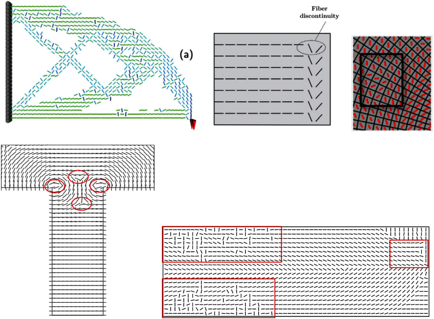
Figure 1: The spatial discontinuity of the fiber angles shown in the literatures [36,39–42]
To overcome the spatial discontinuity and singularities, the NURBS-based IGA is utilized in [24]. A two-layered fiber angle optimization method called Bi-CFAO is proposed. The fiber angles and the element densities are set as design variables and they are optimized synchronously. The fiber angles are then updated by a user-defined function called the reselection procedure. In [24], the angles in base layers are set as the design variables instead of the angles in all the layers. The fiber angles between different layers are predefined as constants for multi-layered composites which is similar to [43].
The IGA based Bi-CFAO method is effective to generate fiber paths with smaller curvatures compared to the conventional CFAO. However, the previous paper found that even with this nature filtering advantage, the spatial discontinuities still exist in the generated fiber paths.
In order to eliminate the discontinuities, this paper continues to investigate the IGA method based on control points and proposes a more effective angle selection strategy to solve the problem of fiber path discontinuity. A new updating strategy called the modified angle selection procedure is developed. Firstly, the adjacent points in the abrupt changing areas are connected to lines and the lines are classified into edge-to-edge lines and non-edge-to-edge lines. The fiber angles in the non-edge-to-edge lines are interpolated by the angles around them. Then, the design domain is separated by edge-to-edge lines into subdomains. The angles in the biggest subdomain remains and the angles in the nearby subdomains are updated by flipping 90°. The biggest subdomain will be enlarged by the updated nearby subdomains, and new iterations are performed until all the subdomains are updated. After the updating process the continuous curve fiber paths are obtained. The locations and geometries of the discontinuous points are involved in the new updating strategy. More complex situations can be solved compared with the original angle selection procedure. The new method is extended to multi-layered cases.
This article is structured as follows: basic theories are introduced in Section 2, including the NURBS based IGA, the modified CFAO fiber angle optimization. In Section 3, the proposed control-points based XBi-CFAO method for the typical elasticity problems are presented. The new angle updating process is introduced. In Section 4, effectiveness and stability of the proposed method is illustrated by three benchmark problems. The article concludes with a discussion in Section 5.
In this section, the basic theories are introduced. The NURBS-based IGA method is applied to calculate the structure response, the fiber angle optimization for single layer and two-layered composites are both based on the CFAO method, the design variables are updated by using the MMA algorithm [44].
2.1 The Overview of NURBS Based IGA
In IGA approaches [22], a unified mathematical form for both CAD and CAE models is performed, by utilizing the same NURBS basis functions to describe the geometry and to construct the space for structural responses.
Non-uniform rational B-splines (NURBS), constructed from B-splines, is a standard technology employed in CAD systems to represent curves and surfaces. NURBS is one of the most thoroughly developed and in most widespread use in both CAD and IGA [22].
To construct B-spline basis functions of order p, a knot vector Π, which consists of n spline basis functions, is defined in the parameter space as
where p is the order of the B-spline. The vector Π is a sequence of non-decreasing real numbers representing parametric coordinates of a curve. The interval [η1, ηn+p+1] is called a patch, and the knot interval [ηi, ηi+1) is called a span.
The B-spline basis functions are recursively defined following the Cox-de Boor formula [45]
It is observed that the B-spline basis functions constitute a partition of unity.
In two-dimensional cases, the B-spline basis functions are constructed as tensor products
where Bi,p(ξ) and Bj,q(η) are univariate B-spline basis functions of order p and q, corresponding to knot vectors Π = {ξ1, ξ2, …, ξm+q+1} and Ψ = {η1, η2, …, ηn+p+1}. Given a set of control points Pi,j, a bivariate B-spline surface is obtained as the tensor product of two B-spline curves
where Pi,j is the (i, j)-th control point in the design space. The patch for the surface is now the domain [ξ1, ξn+p+1] × [η1, ηm+q+1].
Assigning a positive weight ωi to each basis function of the B-splines then we get the NURBS basis functions. It is easy to find that, if the weight values are all equal, the NURBS becomes B-splines. When describing the circles, cylinders, cones, and spheres, the weight values are not all equal [46].
The two-dimensional NURBS basis functions are constructed as
where ωi,j is the weight value of the control point Pi,j in the NURBS surface. The weight values of rational basis functions are not equal for the circle, cylinder, cone, and sphere, but could be all equal when describing some other geometries. If the weights are all equal, the NURBS becomes B-splines. More details are referred to [8,22,46].
To represent a NURBS surface with the control points Pi,j, i = (1, 2, …, n), j = (1, 2, …, m), orders of p and q, the parametric form is
In NURBS based IGA, these NURBS basis functions are applied for both shape representation and physical field approximation. It is noted that Pi,j can represent the control points for describing the geometry as well as other physical quantities that is associated with [22,27,47]. For example, the displacements, the stress and strain, the design fiber variables like fiber angles and material densities.
In this paper, the fiber angles and material densities are simultaneously optimized using the Bi-CFAO method. The densities and fiber angles are both set as design variables. And the optimization process is similar to the conventional CFAO. The fiber angles update continuously during the iteration.
In the Bi-CFAO approach [24], the composite plates are consist of two layers of curved fibers. The fibers in the upper layer are set as perpendicular to the ones in the bottom. Firstly, the IGA model is constructed with predefined material parameters, displacement constraints and force constraints in the design domain. Then the structure response and the objective function are calculated. After that, the sensitivity computations are accomplished and the design variables are optimized using the MMA approach. The difference between the Bi-CFAO and the common CFAO is the layer numbers. The element fiber angles in the Bi-CFAO represents two layers, but the element fiber angles in the common CFAO represents one layer. The element stiffness matrix should be defined as the sum of the two layers as well as the analysis of the sensitivities of the fiber angles in Bi-CFAO. The fiber paths of the two layers should be generated related to the fiber angles respectively. After the fiber angle optimization, a selection process is applied to update the fiber angles and to guarantee the fiber paths are smooth.
3 Definitions of IGA Based XBi-CFAO
3.1 Definition of the Optimization Problem
In this study, the general compliance minimization problem is considered. The optimization problem is defined as
where θ is the element angle vector, ρ is the element density. N is the element number, c is the compliance, u, K and f are the global displacements, global stiffness matrix and force vectors, respectively, f is the volume constraint. V0 is the domain volume. V(ρi) is the i-th element volume (area in 2D problems). The material density optimization procedure is based on SIMP approach [48,49]. In this paper, the penalization factor is 3. If the solid design domain is considered (this means that, only fiber angles are optimized while the design domain is all filled with solid materials), all the element densities should be set as 1. The θmin and θmax are set as –90° and 90°, respectively. The ρmin and ρmax are set as 0.001 and 1, respectively.
As a common practice for numerical implementation purposes in the literature [48], a filter is applied to avoid the checkerboard patterns. In the present work, the filtering form is taken as
where
The design variables are updated by a set of elements that has the center-to-center distance smaller than the filter radius rmin, and Hi is a weight factor defined as
where Є(i, j) is the distance between element i and j.
The plane-stress quadrilateral element is used in this study. The orthotropic material element stiffness matrix is:
where the 2-D integration is performed over each element domain A, NL is the total number of layers, B is the strain-displacement matrix. D is the element orthotropic constitutive matrix.
In the multi-layered cases, the fiber angles in other layers are set as different from the angles in the base layer [43,50]. Similar to the 2-layered cases, the angle difference between layer j and the base layer is set as constants α. Which can be represented as
The orthotropic material with angle θi has the elastic matrix calculated as
where D0 is the original elastic matrix, T is related to the fiber angle θ and it is the transformation matrix [19,20].
where Ex and Ey are the Youngs modulus, Gxy is the shear modulus, vxy and vyx are the Poisson’s ratios.
3.2 Control-Point Based XBi-CFAO
In the isogeometric Bi-CFAO procedure, the general numerical analytical method FEM is replaced by the NURBS-based IGA. The NURBS basis functions are directly used in structural analysis as shape functions. Hence, a variable x (e.g., density, fiber angle, displacement, or stress) whose parametric coordinate is x (η, ξ) can be evaluated from the control point values
where Ni is the basis function of the i-th control point influencing the position of (η, ξ), and Pi is the corresponding variable value of the related control point.
The j-th layer elementary stiffness matrix Kej can be calculated as
where
The ‘‘NURBS elements’’ play the dominant role in IGA, and this is similar to the character of the elements in FEM. To be exact, they are called the ‘‘spans’’ in IGA [22]. A patch is a local domain of B-spline parametric space. The physical model of the structure is constructed by these patches, like it is constructed by elements in the FEM. In this paper, we call the ‘‘patches’’ elements, for the sake of simplicity.
As the physical models are attached to the control points and represented by the NURBS basis functions. The design variables could be optimized on the control points as well as located at the center of the elements. The former is called control point-based and the latter is called the element-based ITO.
In the element-based IGA topology and fiber angle optimization, the element density and fiber angle are represented by the values at the element center, which is calculated by
where ec denotes the center of the e-th element, pe is the control point set that influences element e, pek is the k-th control point of pe, and Npek(ec) is the NURBS basis function of control point pek corresponding to the center of element e. The
In the minimum compliance problems, the compliance sensitivity for element density can be written as
The derivatives of compliance for the element fiber angles are obtained as
However, the design variables should be changed from elemental to control point variables in the control point-based ITO. Therefor an additional job should be performed during sensitivity analysis. The sensitivities of the objective function c for respect to the density of control points are written as
And the sensitivity of fiber angle on a control point is calculated as
The derivation in the chain derivation process can be written as
where x denotes density or fiber angle.
There are series of methods such as the method of moving asymptotes (MMA) [44], the sequential quadratic programming (SQP) [54], and the optimality criteria method (OC) [48], are competent to solve the gradient-based topology and angle optimization problems. In this work, the MMA optimizer is adopted. The convergence criteria are set as the density and fiber angles of the current iteration is less than the preset convergence error δ or the iteration number is greater than the max iterations number Nt (in this paper, δ = 0.0001, Nt = 40).
Fig. 2 shows the flowchart of the main procedure. The optimization procedure for optimizing the fiber angles and element densities is shown in the left part of the figure. It can be outlined as follows:
Step 1. Initialize the design domain, boundary conditions, and optimization parameters.
Step 2. Define NURBS spaces and IGA models.
Step 3. Calculate the element stiffness matrixes with the element densities and fiber angles.
Step 4. Assemble the global stiffness matrix.
Step 5. Analyze with IGA.
Step 6. Calculate the sensitivities of the control points.
Step 7. Optimize the design variables with the MMA process.
Step 8. Iterate until the convergence.
After the fiber angle optimization process, the fiber paths are generated and updated if the fiber angles are changing abruptly. The detailed fiber path updating algorithm is introduced in the next section and the flowchart is shown in the right part of Fig. 2.
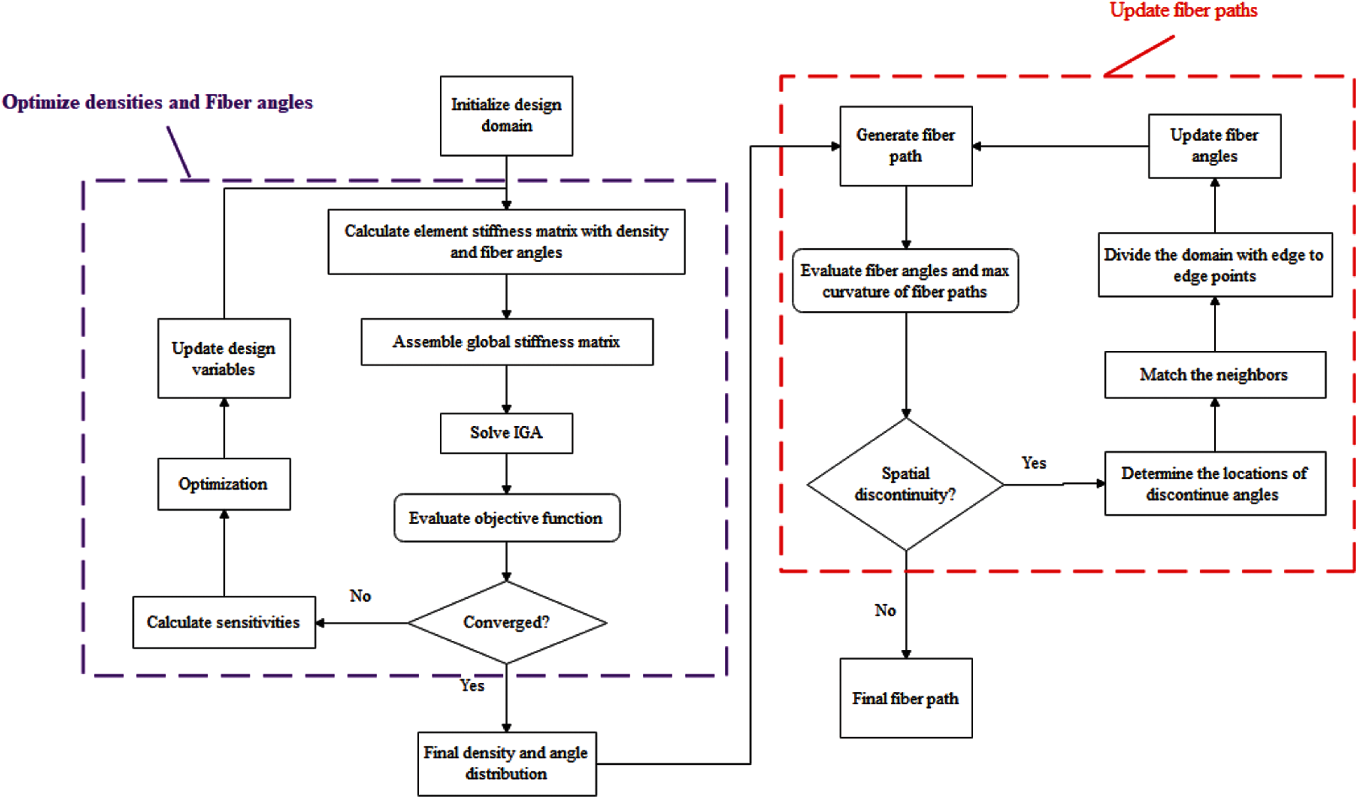
Figure 2: The flowchart of IGA based XBi-CFAO optimization procedure
3.4 The New Selection Process for Smooth the Fiber Path
As is mentioned in our former work [24], the path generation procedure is performed applying the MATLAB function stream slice. The path generation procedure can plot the fiber paths during or after the optimization iterations.
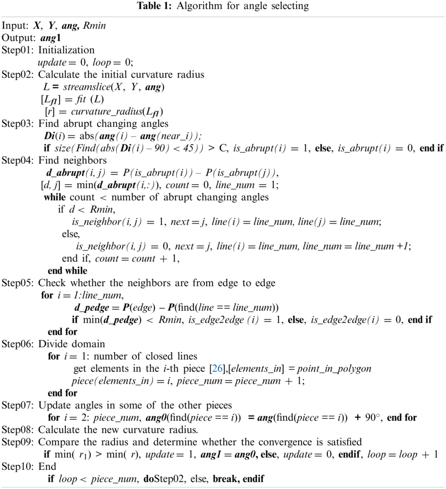
As introduced in Section 1, a new updating strategy called the modified angle selection procedure is developed in this paper to handle the discontinuous of the fiber paths. Tab. 1 shows the new selection progress. The Matlab functions like stream slice, abs, sum, min, and find are applied in a loose form for the sake of simplification. Three user-defined functions are used: fit, curvature_radius, and point_in_polygon in the algorithm. The former two user-defined functions are the same as our former work [24]. The detailed algorithm of the third user-defined function in step 06 is referred to literature [26].
The sketch map of these steps is shown in Fig. 3. The first row with four pictures shows the schematic diagram. The second row shows the steps listed in Tab. 1. The last row shows the detailed process flow chart of some steps.
It is easy to find that the first picture in the first row shows the abrupt changing angles in the design domain. We should find these angles first. The first picture in the third row shows how to find these angles. The abrupt angles can be determined by the size number of Di close to 90°. The number C is the biggest lever set size number (C is set as 8 in this paper).
As shown in the second picture of the first row, the singular angles could be interpolated according to the surrounding angles, because their neighbors are uniformly smooth. However, the abrupt changing angles near the edge-to-edge line could not be smoothed by the filtering technique. The angles are continuous and uniform in each side of the edge-to-edge line. And these angles are divided into two parts by the edge-to-edge line. Flipping the angles by 90° in one side can make the angles more continuous and uniform in both sides.
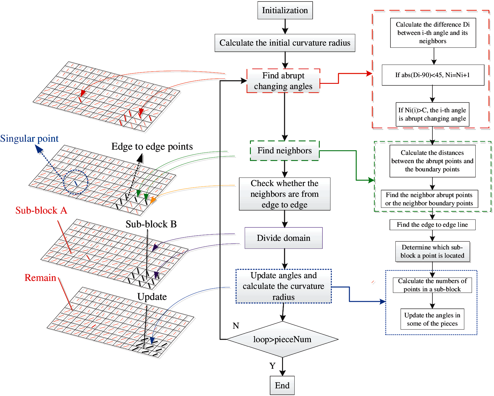
Figure 3: Schematic diagram of the selecting strategy in the XBi-CFAO
Therefore, we should classify the abrupt changing angles into two kinds, including the angles in an edge-to-edge line and the angles in a non-edge-to-edge line (including the singular angles). To classify the abrupt changing angles, all the points located at the abrupt changing angles and the points located in the boundaries of the design domain should be taken into account. The distances between all these boundary-points and the abrupt changing points should be calculated to find the neighbors of each abrupt changing point. Then we should connect the local neighbored points into a line. A minimum spatial distance Rmin is applied to distinguish whether the point is in the same line. (Rmin is set as twice of the element length). Then we should classify the lines into the two kinds, including the edge-to-edge line and the non-edge-to-edge line. As shown in the second picture in the first row, the blue line located in the dashed blue circle is a typical singular point (non-edge-to-edge line). The black lines are made of the angle points located in the edge-to-edge line.
After the edge-to-edge line is determined, the domain is divided into pieces. It is shown by the red lines and black lines in the third picture in the first row. The edge-to-edge line divides the domain to sub-block A and sub-block B. The angles are set as different groups by the location using a point-in-polygon algorithm [26] to determine which sub-block the element is located in.
We set the largest group of angles remain as the original values and the sub-blocks around the largest group update. As shown in the fourth picture in the first row, the sub-block A has the largest group of the angles so that the fiber angles remain the original angles. The fiber angles flip 90° in sub-block B.
After updating the fiber angles sub-block by sub-block, the minimum radius of curvature of the new paths should be calculated. If the minimum radius is maximized and remains constant or the loop number is bigger than the number of pieces, the updating process will be ended.
As we have described in the former part of this section, the elements are constructed by two layers, and the fiber angles in the two layers are perpendicular to each other. In the updated groups, the fiber angles just like flip from the base layer to the other layer. This fiber angles updating process seems to select an appropriate assembly of the divided pieces to avoid spatial discontinuity of the fiber paths. After this process, most of the local discontinuity may vanish.
In this work, the fiber angles for multi-layered composites are then considered by extending the Bi-CFAO method to multi-layered cases. The main difference between the multi-layered and two-layered laminates is the construction of the element stiffness matrix. For the sake of simplicity, the manufacturing constants are not considered in the present paper.
In this section, numerical results generated with the proposed XBi-CFAO method are presented. The mechanical parameters for the composite material are assumed as Ex = 1.0, Ey = 0.1, Gxy = 0.02, vxy = 0.3. In the sake of simplicity, the target volumes are V0 = 1 and V0 = 0.8, respectively. In this paper, the fiber angles with and without topology optimizations are both performed. In the V0 = 1 case, they are optimized without changing densities. Both quadratic elements are used for IGA and FEM.
The first example is a typical problem that is frequently applied in NURBS-based IGA topology optimization. As shown in Fig. 4, the design domain is a quarter annulus, which with the inner radius r = 1 and outer radius R = 2. A horizontally loaded concentrated force F is at the left-top corner. The bottom boundary is fixed. The quadratic NURBS element is applied in this example for IGA and the h-refinement is used to generate the finer NURBS meshes.
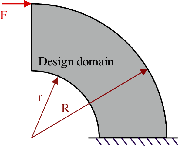
Figure 4: Quarter annulus design problem
Fig. 5 shows the quadratic NURBS elements constructed by the control points. It is noted that, some of the NURBS control points are out of the design domain, which is different from the interpolation type FEM node. The mesh construction process is described in the former work [55]. For a better understanding of the NURBS-based IGA, readers may refer to [22,29,46]. The NURBS element size is 32 × 32 and the control point size is 34 × 34. In this example, a 9-node quadratic element is applied to execute the FEM computing.
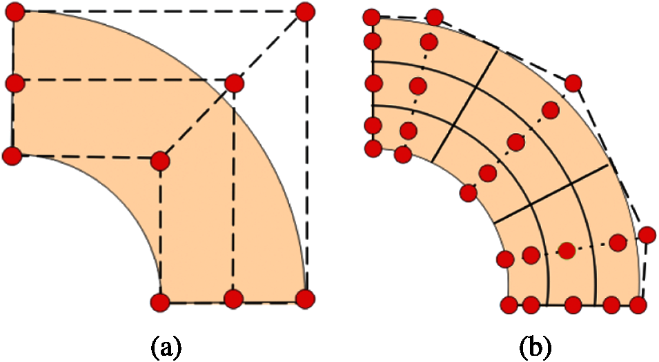
Figure 5: The control points of quarter annulus with (a) 1 × 1 quadratic NURBS element and (b) 3 × 3 quadratic NURBS elements
In this example, three optimizations are accomplished with the different initial angles, which are set as 0°, 45° and 90°, respectively. The phenomenon of fiber angle discontinuity and the selection process is presented firstly. The fiber angle results of the three optimizations are shown in Fig. 6. The abrupt changes of fiber angles are found in all the results, and the discontinuity points partitioned the design domain into 2 pieces. The fiber angles in the sub-blocks are mainly continuous with some local singular points. The locations of the abrupt changing angles and shapes of the sub-blocks are different in the three cases. But it should be noted that the fiber angles in the smooth areas are similar to each other.
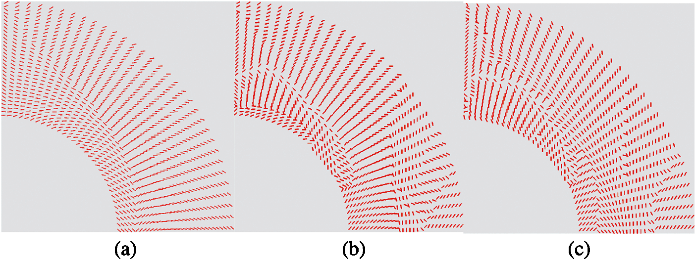
Figure 6: Optimized fiber angles with different initial values (a) θ0 = 0°, (b) θ0 = 45°, (c) θ0 = 90°
The fiber paths are generated using the Matlab function stream slice with discontinuities shown in Fig. 7. The red lines are the paths in the basic layer. The blue lines are the paths in the next layer. The locations of the unsmoothed fiber paths are attached to the abrupt changing angles. The shapes of the fiber paths in the uniformly continuous parts of the sub-blocks are almost the same to each other. The fiber paths with different initial fiber angles seem like several identical paintings whom are torn to pieces in different starting positions. The updating process seems like a restoration for the destroyed paintings. A schematic diagram of the updating process is shown in Fig. 8. It is noted that, during the optimization process, the singular fiber angles exist in the control points, these singular points can be ignored in the selection process. Profit from the NURBS-based IGA, the element angles in these areas are smoothed by the natural NURBS filtering. In the FEM cases, additional filtering should be performed to handle these singular points. The results of the updated fiber angles are shown in Fig. 9 and the updated fiber paths are shown in Fig. 10.
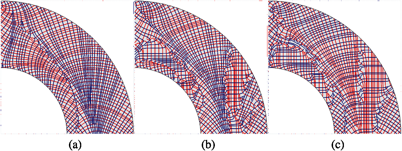
Figure 7: Fiber paths with different initial fiber angles (a) θ0 = 0°, (b) θ0 = 45°, (c) θ0 = 90°
Figure 8: The schematic diagram of updating process
The element fiber angles generated by the IGA and FEM are shown in Fig. 11. It is shown that the fiber angles are similar. The abrupt changing angles are located in the same area, but the line in the FEM is more evident as the differences between the angles located beside the line are closer to 90°. As the angles in the IGA are naturally filtered by the NURBS. The Fig. 12 shows the convergence history of the objective function for IGA and FEM. The objective function numbers for the IGA in the CFAO, Bi-CFAO, and XBi-CFAO are 26.9, 37.9 and 32.7, respectively. And the values in FEM are tiny bigger, they are 27.3, 38.0 and 32.8, respectively. The IGA is more effective to generate uniform smooth fiber angles and to obtain better results of objective functions than FEM.
Figure 9: The updated fiber angles at the control points
Figure 10: The fiber paths generated from the updated fiber angles (a) Layers (θ0) and (θ90), (b) Layers (θ45) and (θ–45)
Figure 11: The element angles generated by IGA and FEM (a) IGA element angle distribution, (b) FEM element angle distribution (c) IGA element angles, (d) FEM element angles
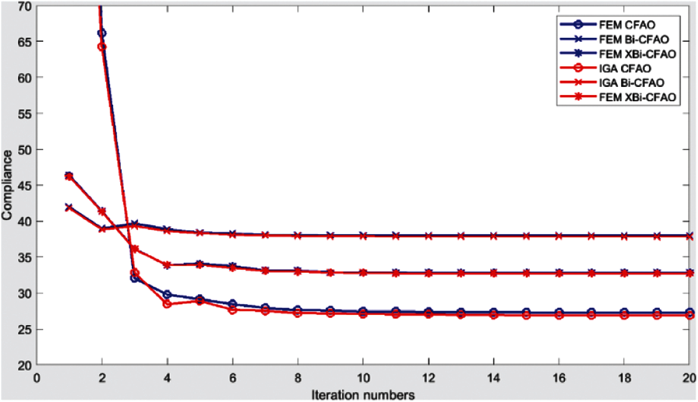
Figure 12: The convergence of the objective function using IGA and FEM
Fig. 13 shows the synchronous optimization of the topology and fiber angles. In the XBi-CFAO, the fiber angles and topology can be optimized synchronously and the fiber angles can be optimized alone as well. It is found that, in Bi-CFAO and XBi-CFAO, the optimized results for the fiber angles and fiber paths may differ in different areas of the design domain, but the locations and shapes of the abrupt areas are not near or attached to the void elements.
However, the results for conventional CFAO, shown in Fig. 14, are near to the void areas. The shapes of the fiber paths are different in the void areas, compared to the paths located in the solid areas [19]. The Bi-CFAO and XBi-CFAO are not as sensitive as the CFAO to the topology changes. As shown in Figs. 10 and 13, the shapes of the updated fiber paths for the target volumes V = 1 and V = 0.8 in the remained design domain areas are the same.
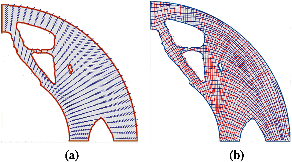
Figure 13: The topology and fiber paths for target volume 0.8 using XBi-CFAO (a) The updated fiber angles, (b) The fiber paths
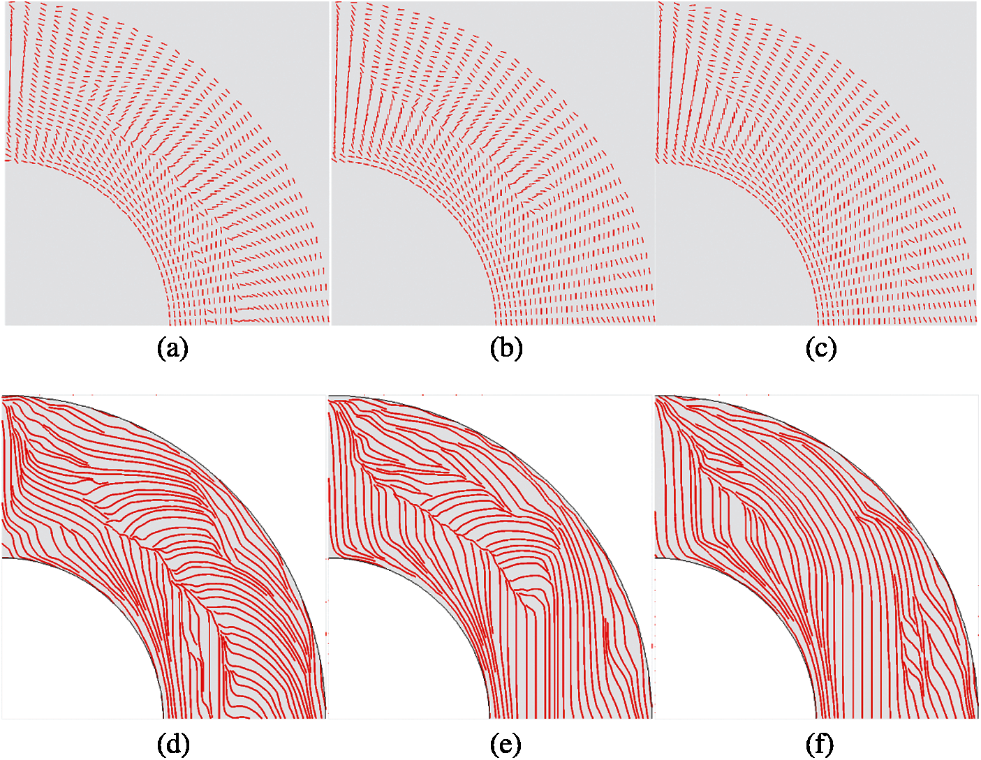
Figure 14: Optimized fiber angles and fiber paths for single layer using CFAO that with different initial values (a) θ0 = 0° (b) θ0 = 45° (c) θ0 = 90° (d) θ0 = 0° (e) θ0 = 45° (f) θ0 = 90°
The three-layered composites are optimized as well. The results are shown in Fig. 15. The red lines are corresponding to the base layer θ0, the blue lines are corresponding to the layer θ45, the green are corresponding to the layer θ–45. The optimized fiber paths in Fig. 15c are similar with Fig. 10a. The results show that, the fiber paths for three-layered cases can be smoothed using the XBi-CFAO method as well as two-layered cases.
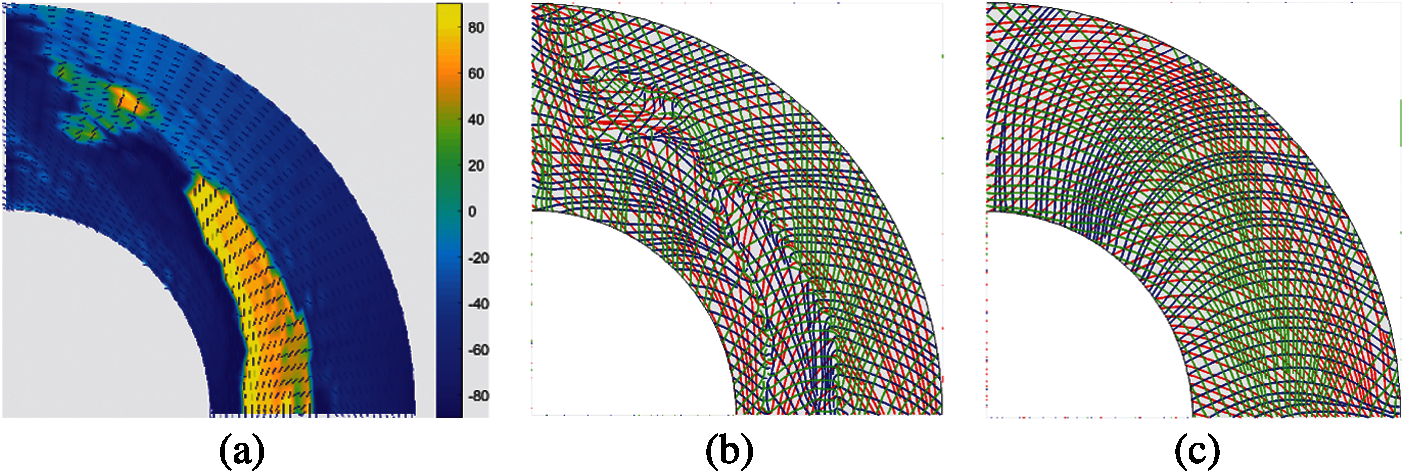
Figure 15: The fiber angles and fiber paths by XBi-CFAO (a) Fiber angles in base layer by XBi-CFAO (b) Fiber paths (c) Updated fiber paths
As shown in Fig. 16, the convergence of the objective functions using conventional CFAO (blue lines), Bi-CFAO (red lines) and the extended Bi-CFAO (green lines) for single layer, bi-layered and three-layered composites are compared. The total thicknesses for the IGA models are set as equal in these problems for the sake of fairness. The results indicate that the objective functions of the Bi-CFAO for two layers are bigger than the others. The conventional CFAO for single layer yield better objective functions than the other two. This is mainly because the restricted condition in element angle combinations for the conventional CFAO is the weakest and the restricted condition for the Bi-CFAO is the strongest. Suppose the best fiber angle for an arbitrary element is 0°. The fibers in the three layers in conventional CFAO could all be 0°. But for Bi-CFAO, one could be in 0°, the other should be in the 90°, which is in the most opposite direction to the best field. For the extended Bi-CFAO, one fiber could be along the direction of 0°, the other two fibers may have a ‘component’ in the best direction of 0°. However, the effect of the manufacturing defects induced by the big curvature is not considered during the objective function computing process. The minimum curvature radius for CFAO is equal to the minimum length of the element (refer to Fig. 14), while the minimum curvature radius for Bi-CFAO is equal to 10 times of the minimum length of the element (refer to Fig. 10b). The Bi-CFAO and XBi-CFAO results are more benign for manufacturing than CFAO.
As in practice, the composite structures are designed as multi-layered with predefined layer angles for the considerations of structure reliability and the convenience of manufacturing. The XBi-CFAO for multi-layered composites is beneficial to the angle optimization for multi-layered structures, because the XBi-CFAO method is capable of obtaining smooth and continuous fiber paths. The XBi-CFAO is stable, but the two-layered composites have larger objective functions than the single-layered composites optimized by the conventional CFAO and the three-layered plates optimized using the XBi-CFAO. This is because the objective functions are calculated without consideration of the manufacturing defects. The fiber paths generated by the Bi-CFAO and the XBi-CFAO for perpendicular multi-layered cases are smooth. This makes the Bi-CFAO and the XBi-CFAO method more promising for fiber angle optimization than the conventional CFAO.
The results also show that all the objective function numbers are about 32 for CFAO (the green lines), 44 for Bi-CFAO (the red lines), and they are 38 for XBi-CFAO (the green lines). The updated fiber paths and fiber angles are nearly the same. This implies that the optimization results depend on the initial design. The optimized compliance are close [19].
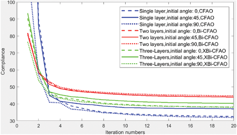
Figure 16: Convergence of the objective function using conventional CFAO, Bi-CFAO and XBi-CFAO target volume 0.8
This example is a 2 × 1 rectangular overhanging beam shown in Fig. 17. The bottom left point is fixed. The midpoint of the bottom line is fixed along the perpendicular direction. An in-plane force f = 1 is applied at the middle point of the right line. The IGA model is then constructed using B-spline, as the weights are all equal. The model is 64 × 32 elements and 66 × 34 control points.
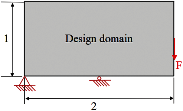
Figure 17: Overhanging beam design domain
The initial fiber angles are set as 0° for each element. The fiber angles in the first few iterations and the final iteration are shown in Fig. 18. It is found that the fiber angles convergence quickly in the first few iterations. The fiber angle optimization procedure provides a segmented continuous fiber angle distribution. In Fig. 18e, the fiber angles are not uniformly continuous, an obvious spatially discontinuous appears in the midline of the design domain and some local spatially discontinuity are also found in other areas in the design domain.
After the optimization procedure, the fiber paths are generated by the fiber angles using the Matlab function stream slice which is mentioned in the former section, and they are shown in Fig. 19. The fiber paths in the two layers are shown together. The red lines represent the fiber paths generated from the fiber angles of the final iteration shown in Fig. 18e. As predefined in the former section, the paths in the other layer are perpendicular to the base layer in XBi-CFAO. The angles in the upper layer (θ90) are calculated by adding 90° to the angles in the base layer (θ0). The blue lines represent the fiber paths generated from (θ90). Without any treatment, the fiber paths may contain discontinuous parts in the design domain, and the location of the discontinuous parts are corresponded to the angle discontinuous areas.
As shown in the Fig. 18e, in the middle of the design domain, the fiber angles flip about 90° in the discontinuous areas. As a result, the fiber paths fold 90°, in the same areas (the red lines in the middle of the domain from top to bottom in Fig. 19. The 90° flipping phenomenon is reported in some of the references [24,42].
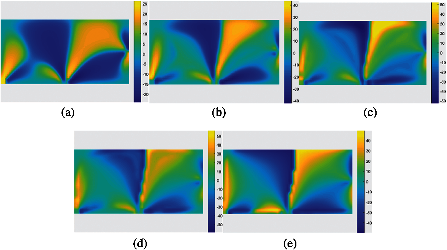
Figure 18: Fiber angles at the element centers in the base layer optimized by Bi-CFAO. (a) 1 iteration (b) 2 iterations (c) 3 iteration (d) 4 iteration (e) 20 iteration
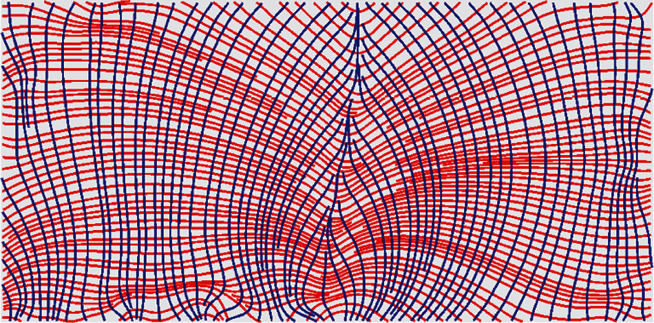
Figure 19: Fiber paths generated from the fiber angles of the final iteration, the red lines. Are corresponding to the base layer (θ0), the blue paths are corresponding to the next layer (θ90)
The fiber angle selection process is performed to accomplish the fiber angle updating procedure. In this example, the middle line partition the design domain into two areas. The abrupt change of the fiber angles and the edge-to-edge line is so easy to find out. The local singular angles and the edge-to-edge line are shown in Fig. 20. The fiber angles in the left are remained and the ones in the right flip 90 degrees. Fig. 21 shows the smoothed fiber angles. After this treatment, the fiber angles are uniformly continuous without any abrupt changing. It is noted that a filtering for the angles is not necessary to smooth the local singular angles located at the not edge-to-edge lines benefit by the nature filtering of the NURBS-based IGA.
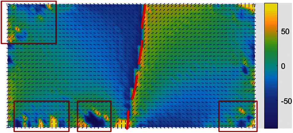
Figure 20: The edge-to-edge line (red line) and the local singular angles in the control points (located in the rectangles)
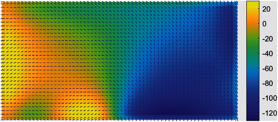
Figure 21: The updated fiber angles
As shown in Fig. 22, the updated fiber paths are smoother and without any sharp turn. Not like the CFAO method, the fiber paths generated by the Bi-CFAO method are not along with the principal stress trajectories, readers are referred to other examples in the former work [24]. It is interesting to find that, the fiber paths generated by the fiber angles of θ0±45° of are along with the principal stress trajectories. These new fiber paths are more recognizable, similar to the conventional multi-layered laminates, the related layers θ0±45° are at the direction of ±45° to the base layer. The new layers are shown in Fig. 23.
It is found that, there are two ways to get the new layers, the first one is to rotate the generated fiber angles in the base layer, the second way is set the values of the Young’s moduli as E1 = 0.1, E2 = 1.0.
The elasticity modulus D11, which is the first entry in the matrix D in Eq. (13) in the former section, are shown in Fig. 24. The parameters D11 corresponding to fiber angles for Bi-layer and single layer are represented using blue and red points, respectively. It is shown that, in the direction of ±45°, the elasticity moduli are bigger than the other directions for the blue points. In contrast, the maximum value appears in the x direction for the red points. This indicated that, for Bi-CFAO the maximum stiffness direction is along the ±45°. The optimization for minimizing compliance problems
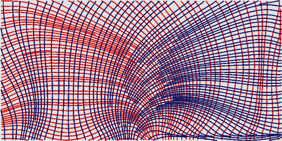
Figure 22: The fiber paths generated from the updated fiber angles, the red lines are corresponding to the base layer θ0, the blue paths are corresponding to the next layer θ0+ 90
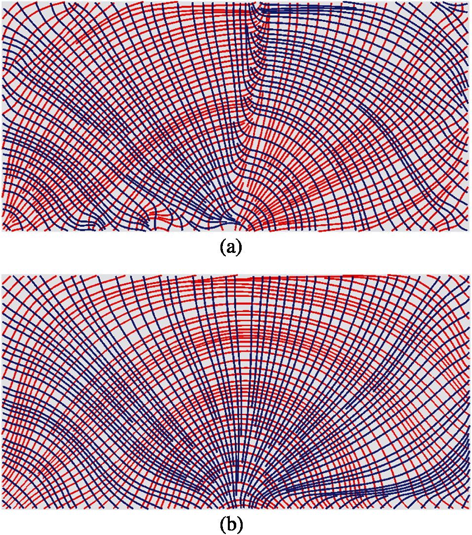
Figure 23: The fiber paths generated from the angles before and after updating process, the red lines are corresponding to the layer θ0 + 45°, the blue paths corresponding to the layer θ0 – 45° (a) Fiber paths generated from θ0±45° (b) Fiber paths generated from updated θ0±45°
The single-layer fiber angles and fiber paths are optimized and shown in Figs. 25 and 26. The fiber angles are optimized using CFAO, the fiber paths are generated with the fiber angles without any treatment. The directions of the fiber paths in most of the cases are along with the principal stress trajectories.
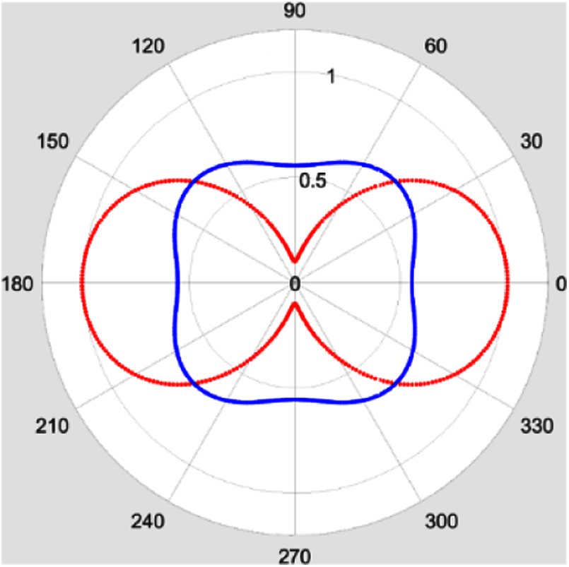
Figure 24: The parameters of bi-layer and single layer elastic matrix corresponding to fiber angles, the red points represent single layer, the blue points represent bi-layer
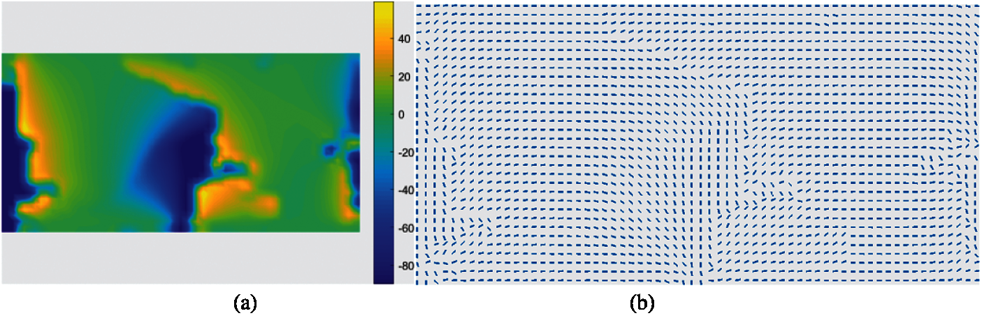
Figure 25: Fiber angles at the element centers in the final iteration of optimization using CFAO (a) Distribution of angles, (b) Fiber angles
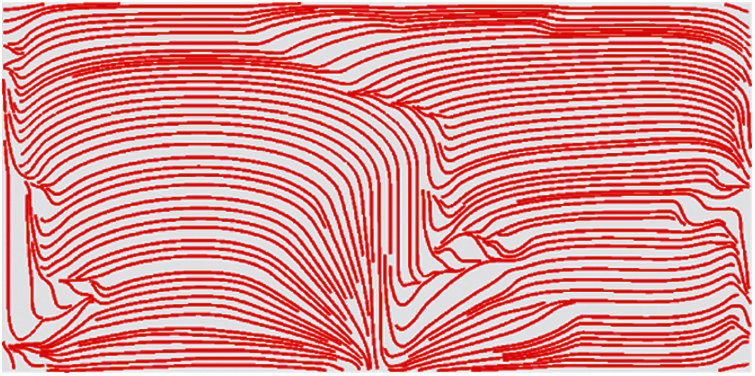
Figure 26: Fiber paths generated after the final iteration of optimization using CFAO
For instance, a three-layered case is studied and the fiber angles and fiber paths are optimized using the extended Bi-CFAO. The fiber angles in the base layer are set as design variables, and the angles in the other two layers are set as flip 45° and –45°, respectively. The optimized fiber angles in the base layer are shown in Fig. 27. The base layer fiber angles show that the partitioned areas of fiber angles are found as well as the former ones. The abrupt angle changes are similar to the bi-layered cases. Some of the fiber angles flip 90 degrees in the boundaries of each sub-block area. The fiber paths generated from the fiber angles are shown in Fig. 28 without any treatment. The directions of the fiber paths in the base layer in most of the cases are along with the principal stress trajectories, as shown by the red lines in Fig. 28.
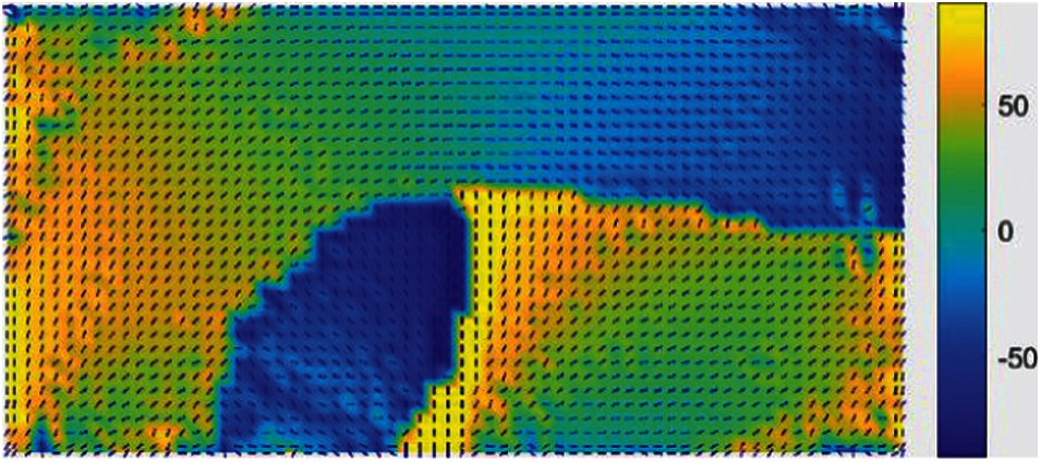
Figure 27: The fiber angles at the control points by extend the Bi-CFAO to three-layered VSLs
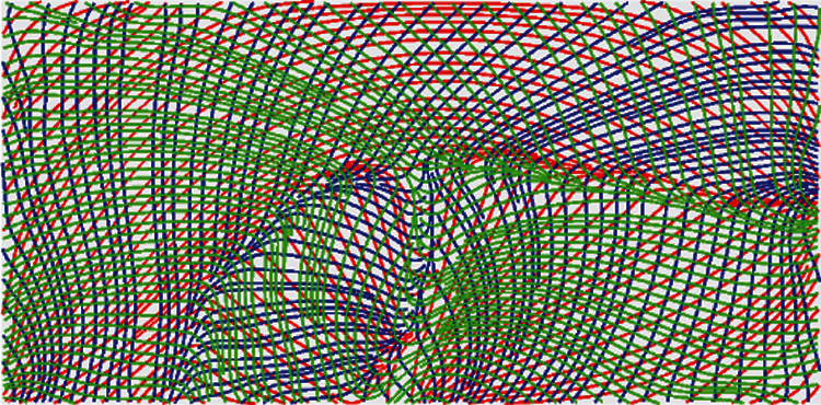
Figure 28: The generated fiber paths, the red lines are corresponding to the base layer θ0, the blue paths corresponding to the next layer θ0+ 45, the green paths corresponding to the next layer θ0 – 45
The smoothed fiber paths are shown in Fig. 29. The fiber paths in the base layer are updated to the same result in bi-layered cases, see the red lines in Fig. 23b. The other two layers are smoother than the ones in Fig. 28. It is noted that, the fiber paths in the right-bottom areas have been changed to perpendicular to the original lines. Which is associated with the selection process, which choose the perpendicular angles to replace the original angles to avoid discontinuity.
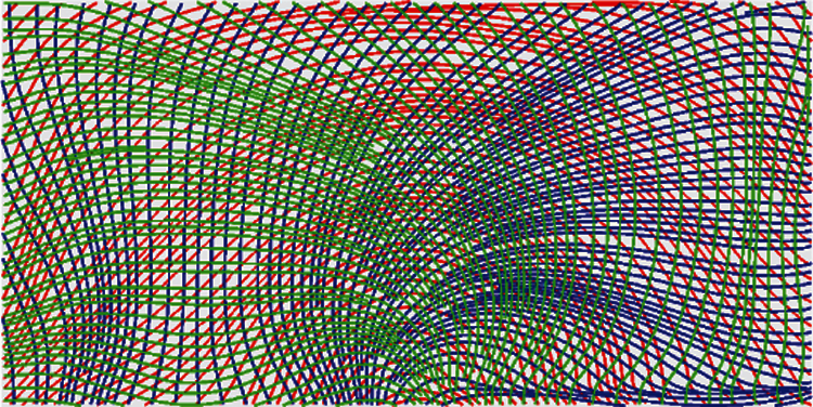
Figure 29: The updated fiber paths using the selection process, the red lines are corresponding to the base layer θ0, the blue paths corresponding to the next layer θ0+ 45, the green paths corresponding to the next layer θ0 – 45
This example is another benchmark problem utilized in NURBS-based IGA topology optimization. The design domain is shown in Fig. 30. A 64 × 32 NURBS element IGA model is constructed with 66 × 34 NURBS control points. It is noted that, as the weights are equal, the NURBS degenerate into B-Spline.
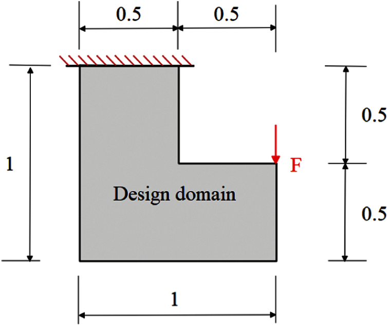
Figure 30: L beam design domain
In this example, we investigate the effects of the angles between layers in the multi-layered cases. As we know, the conventional laminates are constructed by multi-layered panels at different angles [23,57]. The fiber angles of three and four layers are studied. The initial angles in this example are set as 0°.
In the three-layered cases, the angles between the base layer and the next layer (θL1 – θL0) and angles between the base layer and the other layer (θL2 – θL0) are set as different. Six cases are calculated. The angles between θL1 and θL0 are 15°, 22.5°, 30°, 15°, 22.5°, 30°, respectively. The angles between θL2 and θL0 are –15°, –22.5°, –30°, –75°, –67.5°, –60°. The former 3 cases are mirroring cases and the latter 3 cases are perpendicular cases, respectively.
In the four-layered cases, another layer with the angle of 45° is added to the three-layered cases. The angles between layer (θL3) and layer (θL0) are 45° (θL3 – θL0 =45°).
Some of the fiber angle and fiber path results for 4 layers are shown in Fig. 31. The perpendicular and mirror cases for 3 layers are shown in Fig. 32. As shown in Fig. 32a, the red lines are the paths generated by the angles in the base layer, and the blue and green lines are the paths generated by the other two layers. The angles between the red lines and the blue lines are 60°, the angles between the red lines and green lines are 30°. Fig. 32b shows the paths generated in the other two layers. The proposed selection process is based on the assumptions that the angles of the two layers are perpendicular. For the multi-layer cases, if two of the layers are perpendicular, then the assumptions are tenable. In this case, the angles in the perpendicular layers can flip 90° to smooth some of the paths. The fiber paths in (b) are perpendicular. Hence, the fiber angles in (b) can be smoothed using the proposed selection process. The paths in mirror cases are shown in Fig. 32c and 32d. The angles between the red lines and blue lines are 30°, the angles between the red lines and green lines are −30°. The angles between blue and green lines are 60°. In this case, the assumptions are not tenable. As shown in (d), the fiber paths will remain unsmooth even if the angles in some of the areas flip 90° or 60°. The proposed angle updating process is not effective for the mirror cases. The selection process for 3-layered perpendicular cases is presented in Fig. 33.
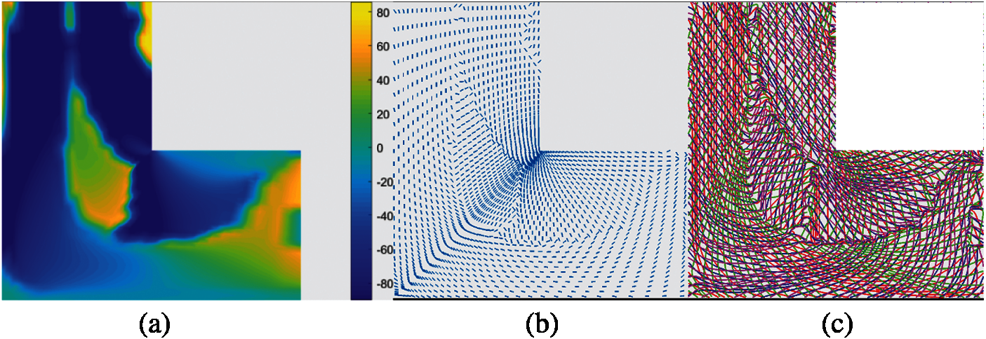
Figure 31: The fiber angles and paths in 4-layered mirror layers (a) The angle distribution, (b) Angles in the base layer, (c) The fiber paths
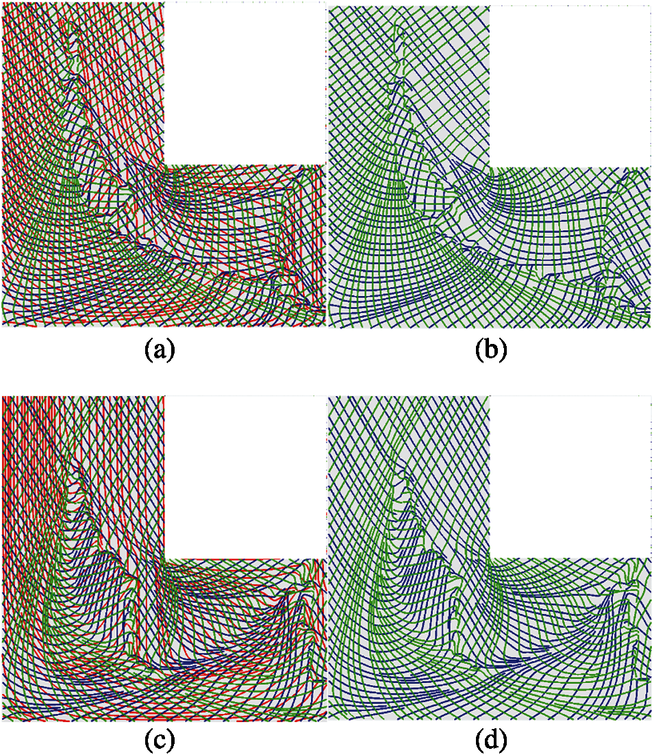
Figure 32: The 3 layers paths of perpendicular and mirror cases, (a) Perpendicular paths of 3 layers, (b) Perpendicular paths of the other 2 layers, (c) Mirror paths of 3 layers, (d) Mirror paths of the other 2 layers
The convergence of the objective functions using the extended Bi-CFAO for 3-layered and 4-layered layers are shown in Fig. 34. The blue and red-colored lines are perpendicular and mirror layers, respectively. The solid and the dashed lines are 4-layered and 3-layered cases, respectively. The fiber paths angles between two layers are set as 15°, 22.5° and 30°, respectively. Twelve optimizations are performed to study the effects of three factors: the angles between layers, the total number of the layers, and the layout form of the layers (mirror and perpendicular). For conventional multi-layered laminates, the design and optimization for the angles between layers, the thickness of different layers, and the stacking sequence are important design variables. In this example, the similar factors are studied to demonstrate their different effects on the compliances. It is found that, the optimized compliances for all the cases are close to each other. The red lines have smaller compliances than the blue lines.
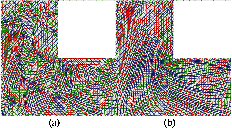
Figure 33: The updated fiber paths using the selection process, the red lines are corresponding to the base layer θ0, the blue paths corresponding to the next layer θ0 + 45, the green paths corresponding to the next layer θ0 – 45 (a) Before updating 3-layered layers, (b) After selection process
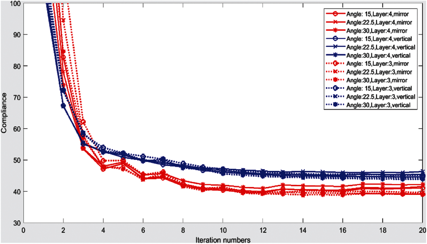
Figure 34: Convergence of the objective function using the XBi-CFAO for 3-layered and 4-layered layers
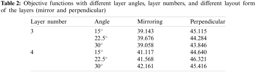
The differences of the objective functions caused by the other two factors are smaller than the layout form factor. Detailed values of the objective functions are listed in Tab. 2. It is shown that the average values for mirror layers and perpendicular layers are 40.45 and 44.94, respectively. The mirror layers have smaller objective function results than the perpendicular ones. The root mean squared errors (RMSE) of the three factors to the objective functions are calculated to represent the effects. The RMSEs of the angles between layers, the total number of the layers, and the layout form of the layers are 0.479, 0.842 and 2.24, respectively. It is noted that, more accurate models should be tested in the future, due to the simplicity of the model in this paper and the absence of the consideration of the manufacturing constraints during the optimization process.
In this paper, an effective multi-layer fiber angle optimization method XBi-CFAO is proposed to optimize the fiber angles and fiber paths for VSLs. In the XBi-CFAO method, the lines made of neighboring abrupt changing angles are classified into edge-to-edge lines and non-edge-to-edge lines. The design domain is divided into subdomains by the edge-to-edge lines and the fiber angles in the divided subdomains are updated to generate smooth paths.
Benchmark examples are presented to illustrate the proposed method. Continuous fiber paths without local small curvatures are obtained retaining the optimal result information of the fiber angles to the maximum extent.
In this paper, the static in-plain problems are studied using the XBi-CFAO method. The out-plain and dynamic problems should be studied in the future. The selection process is based on the assumption that the angles of the two layers are perpendicular. This assumption may limit the usage of XBi-CFAO for multi-layered panels. Complex problems without the perpendicular assumption will be studied in the future as well.
Funding Statement: This research work is supported by the National Key R&D Project of China (Grant Nos. 2018YFB1700803 and 2018YFB1700804), managed by Qifu Wang. These supports are gratefully acknowledged.
Conflicts of Interest: The authors declare that they have no conflicts of interest to report regarding the present study.
1. Gürdal, Z., Olmedo, R. (1993). In-plane response of laminates with spatially varying fiber orientations-variable stiffness concept. AIAA Journal, 31(4), 751–758. DOI 10.2514/3.11613. [Google Scholar] [CrossRef]
2. Gürdal, Z., Tatting, B. F., Wu, C. K. (2008). Variable stiffness composite panels: Effects of stiffness variation on the in-plane and buckling response. Composites Part A: Applied Science and Manufacturing, 39(5), 911–922. DOI 10.1016/j.compositesa.2007.11.015. [Google Scholar] [CrossRef]
3. Hao, P., Yuan, X., Liu, H., Wang, B., Liu, C. et al. (2017). Isogeometric buckling analysis of composite variable-stiffness panels. Composite Structures, 165(3), 192–208. DOI 10.1016/j.compstruct.2017.01.016. [Google Scholar] [CrossRef]
4. Tian, Y., Pu, S., Zong, Z., Shi, T., Xia, Q. (2019). Optimization of variable stiffness laminates with gap-overlap and curvature constraints. Composite Structures, 230(6), 111494. DOI 10.1016/j.compstruct.2019.111494. [Google Scholar] [CrossRef]
5. Lan, M., Cartié, D., Davies, P., Baley, C. (2015). Microstructure and tensile properties of carbon-epoxy laminates produced by automated fibre placement: Influence of a caul plate on the effects of gap and overlap embedded defects. Composites Part A: Applied Science and Manufacturing, 78, 124–134. DOI 10.1016/j.compositesa.2015.07.023. [Google Scholar] [CrossRef]
6. Lan, M., Cartié, D., Davies, P., Baley, C. (2016). Influence of embedded gap and overlap fiber placement defects on the microstructure and shear and compression properties of carbon-epoxy laminates. Composites Part A: Applied Science and Manufacturing, 82, 198–207. DOI 10.1016/j.compositesa.2015.12.007. [Google Scholar] [CrossRef]
7. Esposito, L., Cutolo, A., Barile, M., Lecce, L., Mensitieri, G. et al. (2019). Topology optimization-guided stiffening of composites realized through automated fiber placement. Composites Part B: Engineering, 164(4), 309–323. DOI 10.1016/j.compositesb.2018.11.032. [Google Scholar] [CrossRef]
8. Hao, P., Yuan, X., Liu, C., Wang, B., Liu, H. et al. (2018). An integrated framework of exact modeling, isogeometric analysis and optimization for variable-stiffness composite panels. Computer Methods in Applied Mechanics and Engineering, 339(4), 205–238. DOI 10.1016/j.cma.2018.04.046. [Google Scholar] [CrossRef]
9. Setoodeh, S., Gürdal, Z., Watson, L. T. (2006). Design of variable-stiffness composite layers using cellular automata. Computer Methods in Applied Mechanics and Engineering, 195(9), 836–851. DOI 10.1016/j.cma.2005.03.005. [Google Scholar] [CrossRef]
10. van Campen, J. M. J. F., Kassapoglou, C., Gürdal, Z. (2012). Generating realistic laminate fiber angle distributions for optimal variable stiffness laminates. Composites Part B: Engineering, 43(2), 354–360. DOI 10.1016/j.compositesb.2011.10.014. [Google Scholar] [CrossRef]
11. Xu, Y., Zhu, J., Wu, Z., Cao, Y., Zhao, Y. et al. (2018). A review on the design of laminated composite structures: Constant and variable stiffness design and topology optimization. Advanced Composites and Hybrid Materials, 1(3), 460–477. DOI 10.1007/s42114-018-0032-7. [Google Scholar] [CrossRef]
12. Stegmann, J., Lund, E. (2005). Discrete material optimization of general composite shell structures. International Journal for Numerical Methods in Engineering, 62(14), 2009–2027. DOI 10.1002/nme.1259. [Google Scholar] [CrossRef]
13. Kiyono, C. Y., Silva, E. C. N., Reddy, J. N. (2012). Design of laminated piezocomposite shell transducers with arbitrary fiber orientation using topology optimization approach. International Journal for Numerical Methods in Engineering, 90(12), 1452–1484. DOI 10.1002/nme.3371. [Google Scholar] [CrossRef]
14. Kennedy, G. J., Martins, J. R. R. A. (2013). A laminate parametrization technique for discrete ply-angle problems with manufacturing constraints. Structural and Multidisciplinary Optimization, 48(2), 379–393. DOI 10.1007/s00158-013-0906-9. [Google Scholar] [CrossRef]
15. Gao, T., Zhang, W., Duysinx, P. (2012). A bi-value coding parameterization scheme for the discrete optimal orientation design of the composite laminate. International Journal for Numerical Methods in Engineering, 91(1), 98–114. DOI 10.1002/nme.4270. [Google Scholar] [CrossRef]
16. Gao, T., Zhang, W., Duysinx, P. (2013). Simultaneous design of structural layout and discrete fiber orientation using bi-value coding parameterization and volume constraint. Structural and Multidisciplinary Optimization, 48(6), 1075–1088. DOI 10.1007/s00158-013-0948-z. [Google Scholar] [CrossRef]
17. Jantos, D. R., Hackl, K., Junker, P. (2020). Topology optimization with anisotropic materials, including a filter to smooth fiber pathways. Structural and Multidiplinary Optimization, 61(11), 2135–2154. DOI 10.1007/s00158-019-02461-x. [Google Scholar] [CrossRef]
18. Jiang, D., Hoglund, R., Smith, D. E. (2019). Continuous fiber angle topology optimization for polymer composite deposition additive manufacturing applications. Fibers, 7(14), 1–21. DOI 10.3390/fib7020014. [Google Scholar] [CrossRef]
19. Xia, Q., Shi, T. (2017). Optimization of composite structures with continuous spatial variation of fiber angle through Shepard interpolation. Composite Structures, 182, 273–282. DOI 10.1016/j.compstruct.2017.09.052. [Google Scholar] [CrossRef]
20. Nomura, T., Dede, E. M., Lee, J., Yamasaki, S., Matsumori, T. et al. (2015). General topology optimization method with continuous and discrete orientation design using isoparametric projection. International Journal for Numerical Methods in Engineering, 101(8), 571–605. DOI 10.1002/nme.4799. [Google Scholar] [CrossRef]
21. Wang, D., Abdalla, M. M., Wang, Z. P., Su, Z. (2019). Streamline stiffener path optimization (SSPO) for embedded stiffener layout design of non-uniform curved grid-stiffened composite (NCGC) structures. Computer Methods in Applied Mechanics and Engineering, 344(3), 1021–1050. DOI 10.1016/j.cma.2018.09.013. [Google Scholar] [CrossRef]
22. Hughes, T. J. R., Cottrell, J. A., Bazilevs, Y. (2005). Isogeometric analysis: CAD, finite elements, NURBS, exact geometry and mesh refinement. Computer Methods in Applied Mechanics and Engineering, 194(39), 4135–4195. DOI 10.1016/j.cma.2004.10.008. [Google Scholar] [CrossRef]
23. Hao, P., Feng, S., Zhang, K., Li, Z., Wang, B. et al. (2018). Adaptive gradient-enhanced kriging model for variable-stiffness composite panels using isogeometric analysis. Structural and Multidisciplinary Optimization, 58(1), 1–16. DOI 10.1007/s00158-018-1988-1. [Google Scholar] [CrossRef]
24. Mei, C., Wang, Q., Yu, C., Xia, Z. (2020). IGA based bi-layer fiber angle optimization method for variable stiffness composites. Computer Modeling in Engineering & Sciences, 124(1), 179–202. DOI 10.32604/cmes.2020.09948. [Google Scholar] [CrossRef]
25. Hassani, B., Khanzadi, M., Tavakkoli, S. M. (2012). An isogeometrical approach to structural topology optimization by optimality criteria. Structural and Multidisciplinary Optimization, 45(2), 223–233. DOI 10.1007/s00158-011-0680-5. [Google Scholar] [CrossRef]
26. Wang, Y., Benson, D. J. (2016). Geometrically constrained isogeometric parameterized level-set based topology optimization via trimmed elements. Frontiers of Mechanical Engineering, 11(4), 328–343. DOI 10.1007/s11465-016-0403-0. [Google Scholar] [CrossRef]
27. Wang, Y., Benson, D. J., Nagy, A. P. (2015). A multi-patch nonsingular isogeometric boundary element method using trimmed elements. Computational Mechanics, 56(1), 173–191. DOI 10.1007/s00466-015-1165-y. [Google Scholar] [CrossRef]
28. Wang, Y., Wang, Z., Xia, Z., Poh, L. H. (2018). Structural design optimization using isogeometric analysis: A comprehensive review. Computer Modeling in Engineering and Sciences, 117(3), 455–507. DOI 10.31614/cmes.2018.04603. [Google Scholar] [CrossRef]
29. Wang, Y., Benson, D. J. (2016). Isogeometric analysis for parameterized LSM-based structural topology optimization. Computational Mechanics, 57(1), 19–35. DOI 10.1007/s00466-015-1219-1. [Google Scholar] [CrossRef]
30. Hao, P., Liu, X., Wang, Y., Liu, D., Wang, B. et al. (2019). Collaborative design of fiber path and shape for complex composite shells based on isogeometric analysis. Computer Methods in Applied Mechanics and Engineering, 354(11), 181–212. DOI 10.1016/j.cma.2019.05.044. [Google Scholar] [CrossRef]
31. Ghiasi, H., Fayazbakhsh, K., Pasini, D., Lessard, L. (2010). Optimum stacking sequence design of composite materials Part II: Variable stiffness design. Composite Structures, 93(1), 1–13. DOI 10.1016/j.compstruct.2010.06.001. [Google Scholar] [CrossRef]
32. Peeters, D., Baalen, D., Abdallah, M. (2015). Combining topology and lamination parameter optimisation. Structural and Multidisciplinary Optimization, 52(1), 105–120. DOI 10.1007/s00158-014-1223-7. [Google Scholar] [CrossRef]
33. Petrovic, M., Nomura, T., Yamada, T., Izui, K., Nishiwaki, S. (2018). Orthotropic material orientation optimization method in composite laminates. Structural and Multidisciplinary Optimization, 57(2), 815–828. DOI 10.1007/s00158-017-1777-2. [Google Scholar] [CrossRef]
34. Hong, Z., Peeters, D., Turteltaub, S. (2020). An enhanced curvature-constrained design method for manufacturable variable stiffness composite laminates. Computers & Structures, 238(4), 106284. DOI 10.1016/j.compstruc.2020.106284. [Google Scholar] [CrossRef]
35. Muramatsu, Y., Shimoda, M. (2019). Distributed-parametric optimization approach for free-orientation of laminated shell structures with anisotropic materials. Structural and Multidisciplinary Optimization, 59(6), 1915–1934. DOI 10.1007/s00158-018-2163-4. [Google Scholar] [CrossRef]
36. Allaire, G., Geoffroy-Donders, P., Pantz, O. (2019). Topology optimization of modulated and oriented periodic microstructures by the homogenization method. Computers & Mathematics with Applications, 78(7), 2197–2229. DOI 10.1016/j.camwa.2018.08.007. [Google Scholar] [CrossRef]
37. Geoffroy-Donders, P., Allaire, G., Pantz, O. (2020). 3-D topology optimization of modulated and oriented periodic microstructures by the homogenization method. Journal of Computational Physics, 401(3), 108994. DOI 10.1016/j.jcp.2019.108994. [Google Scholar] [CrossRef]
38. Groen, J. P., Stutz, F. C., Aage, N., Bærentzen, J. A., Sigmund, O. (2020). De-homogenization of optimal multi-scale 3D topologies. Computer Methods in Applied Mechanics and Engineering, 364(6), 112979. DOI 10.1016/j.cma.2020.112979. [Google Scholar] [CrossRef]
39. Kiyono, C. Y., Silva, E. C. N., Reddy, J. N. (2017). A novel fiber optimization method based on normal distribution function with continuously varying fiber path. Composite Structures, 160(1–2), 503–515. DOI 10.1016/j.compstruct.2016.10.064. [Google Scholar] [CrossRef]
40. Schmidt, M. P., Couret, L., Gout, C., Pedersen, C. B. W. (2020). Structural topology optimization with smoothly varying fiber orientations. Structural and Multidisciplinary Optimization, 62(6), 3105–3126. DOI 10.1007/s00158-020-02657-6. [Google Scholar] [CrossRef]
41. Ferreira da Silva, A. L., Salas, R. A., Nelli Silva, E. C., Reddy, J. N. (2020). Topology optimization of fibers orientation in hyperelastic composite material. Composite Structures, 231(1–4), 111488. DOI 10.1016/j.compstruct.2019.111488. [Google Scholar] [CrossRef]
42. Voelkl, H., Franz, M., Klein, D., Wartzack, S. (2020). Computer aided internal optimisation (CAIO) method for fibre trajectory optimisation: A deep dive to enhance applicability. Design Science, 6(4), 1–26. DOI 10.1017/dsj.2020.1. [Google Scholar] [CrossRef]
43. Brooks, T. R., Martins, J. R. R. A. (2018). On manufacturing constraints for tow-steered composite design optimization. Composite Structures, 204(3), 548–559. DOI 10.1016/j.compstruct.2018.07.100. [Google Scholar] [CrossRef]
44. Svanberg, K. (1987). The method of moving asymptotes—A new method for structural optimization. International Journal for Numerical Methods in Engineering, 24(2), 359–373. DOI 10.1002/(ISSN)1097-0207. [Google Scholar] [CrossRef]
45. de Boor, C. (1972). On calculating with B-splines. Journal of Approximation Theory, 6(1), 50–62. DOI 10.1016/0021-9045(72)90080-9. [Google Scholar] [CrossRef]
46. Piegl, L., Tiller, W. (1995). The NURBS book. Germany, Berlin Heidelberg: Springer-Verlag. [Google Scholar]
47. Cottrell, A., Hughes, T., Bazilevs, Y. (2009). Isogeometric analysis: Toward integration of CAD and FEA. UK: John Wiley & Sons. [Google Scholar]
48. Andreassen, E., Clausen, A., Schevenels, M., Lazarov, B. S., Sigmund, O. (2011). Efficient topology optimization in MATLAB using 88 lines of code. Structural and Multidisciplinary Optimization, 43(1), 1–16. DOI 10.1007/s00158-010-0594-7. [Google Scholar] [CrossRef]
49. Bendsøe, M. P., Kikuchi, N. (1988). Generating optimal topologies in structural design using a homogenization method. Computer Methods in Applied Mechanics and Engineering, 71(2), 197–224. DOI 10.1016/0045-7825(88)90086-2. [Google Scholar] [CrossRef]
50. Brooks, T. R., Martins, J. R. R. A., Kennedy, G. J. (2019). High-fidelity aerostructural optimization of tow-steered composite wings. Journal of Fluids and Structures, 88(7), 122–147. DOI 10.1016/j.jfluidstructs.2019.04.005. [Google Scholar] [CrossRef]
51. Wang, Y., Benson, D. J. (2015). Multi-patch nonsingular isogeometric boundary element analysis in 3D. Computer Methods in Applied Mechanics and Engineering, 293(41), 71–91. DOI 10.1016/j.cma.2015.03.016. [Google Scholar] [CrossRef]
52. Wang, Y., Liao, Z., Ye, M., Zhang, Y., Li, W. et al. (2020). An efficient isogeometric topology optimization using multilevel mesh, MGCG and local-update strategy. Advances in Engineering Software, 139(8), 102733. DOI 10.1016/j.advengsoft.2019.102733. [Google Scholar] [CrossRef]
53. Yin, L., Zhang, F., Deng, X., Wu, P., Zeng, H. et al. (2019). Isogeometric bi-directional evolutionary structural optimization. IEEE Access, 7, 91134–91145. DOI 10.1109/ACCESS.2019.2927820. [Google Scholar] [CrossRef]
54. Boggs, P. T., Tolle, J. W. (1995). Sequential quadratic programming. Acta Numerica, 4, 1–51. DOI 10.1017/S0962492900002518. [Google Scholar] [CrossRef]
55. Xia, Z., Wang, Y., Wang, Q., Mei, C. (2017). GPU parallel strategy for parameterized LSM-based topology optimization using isogeometric analysis. Structural and Multidisciplinary Optimization, 56(2), 413–434. DOI 10.1007/s00158-017-1672-x. [Google Scholar] [CrossRef]
56. Bruyneel, M., Fleury, C. (2002). Composite structures optimization using sequential convex programming. Advances in Engineering Software, 33(7), 697–711. DOI 10.1016/S0965-9978(02)00053-4. [Google Scholar] [CrossRef]
57. Duan, Z., Yan, J., Lee, I., Lund, E., Wang, J. (2019). Discrete material selection and structural topology optimization of composite frames for maximum fundamental frequency with manufacturing constraints. Structural and Multidisciplinary Optimization, 60(5), 1741–1758. DOI 10.1007/s00158-019-02397-2. [Google Scholar] [CrossRef]
 | This work is licensed under a Creative Commons Attribution 4.0 International License, which permits unrestricted use, distribution, and reproduction in any medium, provided the original work is properly cited. |