| Computer Modeling in Engineering & Sciences |
DOI: 10.32604/cmes.2021.017580
ARTICLE
Fail-Safe Topology Optimization of Continuum Structures with Multiple Constraints Based on ICM Method
Beijing University of Technology, Beijing, 100124, China
*Corresponding Author: Jiazheng Du. Email: djz@bjut.edu.cn
Received: 21 May 2021; Accepted: 12 August 2021
Abstract: Traditional topology optimization methods may lead to a great reduction in the redundancy of the optimized structure due to unexpected material removal at the critical components. The local failure in critical components can instantly cause the overall failure in the structure. More and more scholars have taken the fail-safe design into consideration when conducting topology optimization. A lot of good designs have been obtained in their research, though limited regarding minimizing structural compliance (maximizing stiffness) with given amount of material. In terms of practical engineering applications considering fail-safe design, it is more meaningful to seek for the lightweight structure with enough stiffness to resist various component failures and/or to meet multiple design requirements, than the stiffest structure only. Thus, this paper presents a fail-safe topology optimization model for minimizing structural weight with respect to stress and displacement constraints. The optimization problem is solved by utilizing the independent continuous mapping (ICM) method combined with the dual sequence quadratic programming (DSQP) algorithm. Special treatments are applied to the constraints, including converting local stress constraints into a global structural strain energy constraint and expressing the displacement constraint explicitly with approximations. All of the constraints are nondimensionalized to avoid numerical instability caused by great differences in constraint magnitudes. The optimized results exhibit more complex topological configurations and higher redundancy to resist local failures than the traditional optimization designs. This paper also shows how to find the worst failure region, which can be a good reference for designers in engineering.
Keywords: Fail-safe design; topology optimization; multiple constraints; ICM method
With the development of engineering products, a critical controversy in industrial practice arises frequently: a number of measures needs to be conducted to demonstrate product quality and reliability in terms of a specific goal, whereas the structure cost must be controlled within cost limit to ensure the structural economy. Therefore, the concept of structural optimization came into being. In 1904, Michell [1] proposed the famous Michell truss design theory, which was the earliest topology optimization design. As the design complexity increases, structural optimization can be divided into three levels: size optimization, shape optimization, and topology optimization. Topology optimization is more comprehensive compared to the other two. Topology optimization optimizes the objective function by distributing material in the design regions so that it can achieve greater economic benefits and attract more engineering designers’ attention. At present, structural optimization’s research interests mainly focus on continuum structures’ topology optimization [2,3]. Research methodologies include Variable Density Method [4], Homogenization Method [5], Independent Continuous Mapping Method(ICM) [6], Evolutionary Structural Optimization [7], Moving Morphable Components Method(MMC) [8] and so on.
The optimized structure from topology optimization is usually a statically determinate structure whose weight and redundancy decrease greatly. As a result, every member of the structure becomes a critical member. When local failure occurs on one critical member, it is easy to develop into overall failure and then may cause collapses of the entire structure. Although the traditional optimized structure has distinct features such as lighter weight, higher efficiency of material uses, and lower economical cost, this type of structure is lack of security. Especially in high safety requirement engineering field, the structure is extremely unreliable. Therefore, topology optimization considering the concept of fail-safe attracts more and more attention from researchers. The local failures were categorized into two types by Yuan [9]. The first type is that the structure bears an expected extreme load, which causes the local stiffness failure or complete collapse. This type of failure depends on the mechanical properties of the structure. Unexpected accidents cause the second type of local failure, mainly from corrosion, explosion, fatigue, collision and so on. The former failure can be avoided by designing correct size, applying proper load or choosing suitable materials. The failure studied in this paper is the latter. Peng et al. [10] made mention of the fail-safe concept. They concluded that when local failure occurred, the structure designed with fail-safe concept can still survive normal loading conditions.
Since the fail-safe concept was presented, the fail-safe design has been taken into consideration by researchers in engineering application practice. The rectangular failure regions are caused by traditional topology optimization when structural optimization design is carried out. In 1982, Nguyen et al. [11] studied fail-safe optimal design of complex structures and presented a structural formulation for their design problem. In 1998, Bendsøe et al. [12] studied the effect of material property degradation on topology optimization of truss and continuum structures. Jansen et al. [13] put forward a simplified model where several contiguous elements of structure were regarded as a failure region. They combined the fail-safe concept with continuum structure topology optimization and considered uncertain failure position, while shape and size to be certain. But this approach caused the number of local failure regions was the same as the elements’ number so that computational efficiency was hard to accept. In 2016, Zhou et al. [14] developed Jansen’s work and introduced a new arrangement pattern of failure region called Level Laying Strategy which greatly reduced the number of local failure regions and computational cost. And more importantly, this method successfully extended the fail-safe problem to the three-dimensional continuum topology optimization. In 2018, Peng et al. [10] simulated failure working condition based on the research work of Zhou. He clarified some concept used in local failure of structure and solved the fail-safe continuum structure model with the constraint as displacement by using ICM method. In 2019, Du et al. [15,16] used ICM method to solve three kinds of fail-safe continuum structure models with different constraints as stress, displacement, or frequency, and obtained a reasonable optimization structure. However, the work mentioned above is only solved with a single constraint while there is more than one constraint acting at the same time in practical engineering applications. Long et al. [17] aim to make the topology optimization total volume minimizing with multiple compliance as constraints, and his achievement not only took the randomness of the fail regions into account, but also considered uncertain loading magnitude and direction. Lüdeker et al. [18] applied an approach in the fail-safe requirement optimization and reduced the number of failure working conditions within the optimization. In 2020, Li et al. [19] described a damage state of precast concrete barrier for viaducts under failure working condition caused by vehicle collision. In the same year, Ambrozkiewicz et al. [20] proposed a two-stage program based on density optimization for fail-safe design, which improve performance and computational efficiency. Zhao et al. [21] used the T-spline basis functions to propose a new isogeometric topology optimization method. Chen et al. [22] researched a methodology about additional penalization formulation of failure regions, which is capable of fatigue-resistance design for continuum optimization. In 2021, Dou et al. [23] observed the stress constraints’ model in fail-safe structural optimization and found out that the local failure may result in a worse objective function than failing completely. He thought it was necessary to choose the design when the fail-safe designs for degradation or complete failure.
Stress constraints are considered in the optimization to meet the requirement of static strength of a structure. Cheng et al. [24] modified fully stressed criterion to solve topology optimization problems of planar elastomers and thin plate structures with stress constrains. Subsequently, Sui et al. [25] introduced globalization of stress constraints that a global structural strain energy constraint takes the place of local stress constraints to improving computational efficiency, moreover research results are satisfying. Alexander et al. [26] put forward relaxation approach and a unified aggregation with stress as constraints in topology optimization. Chu et al. [27] used stress penalty to deal with localized problems of stress constraints. Wang et al. [28] introduced von Mises stress into fail-safe optimization, this method eliminated unnecessary failure working conditions and get good achievement. Meng et al. [29] used P-norms to convert a large number of stress constraints into a global constraint. Considering multiple material failure criterions, Simonetti et al. [30] carried out continuum structure topology optimization through Smoothing Evolutionary Structure Optimization and Multicriteria Tournament Decision on the basis of stress-strain energy criterion.
To meet the requirement of static stiffness, it is necessary to constrain the displacements at certain locations of a structure. Compared to the stress, the displacement constraint has below different features: the influence scope of the displacement constraint is a globalization constraint and involves in almost every element. The stress constraint is far more difficult to solve than the displacement constraint in the first-order. Also, the number of the displacement constraints is far less than the stress. Sui et al. [31] researched the integrated approach of displacement constraints to solve problem with multiple load cases and multiple displacement constraints. Xie et al. [32] gave the calculation formula of element sensitivities under a topology optimized model with multiple displacement constraints. Zhu et al. [33] studied displacement constraints of multiple load cases in topology optimization of plate and shell structures. Long et al. [34] processed node displacement of bearing surface by KS envelope function to design topology optimization of engineering structure bearing distributed load.
2 Formulation of a Fail-Safe Model on the Basis of ICM Method
Size and location in failure regions are random and uncertain in continuum topology optimization, so it is impossible that the failure working conditions are enumerated and calculated one by one. In order to solve this problem, this paper studies fail-safe topology optimization problems by the Level Laying Strategy proposed by Zhou et al. [14]. Compared to failure regions in other shapes [35], the rectangular failure region has obvious advantages such as easy expression and seamlessly lying in the whole design area. Herein, the rectangular failure region is used in this research. According to the Level Laying Strategy, the failure regions generally are squares lying seamlessly one side after another, then the failure occurs in turn. Locations and sizes of local failure regions are determined in the Level Laying Strategy. Once a failure region fails, it can be taken as a new structural failure working condition. This failure region can be simulated by defining elasticity modulus of some certain locations as 0, which means those failure regions with fixed shape, size and position in a structure are deleted. In the other word, the failure regions are removed from the structure in turn in order to generate different working conditions. Thus, the number of failure regions is same as the number of failure working conditions. Thereafter the uncertain structural failure problem is transformed into a certain multiple working conditions problem. The design variables in topology optimization with local failures can be expressed as follows:
where D is the design region.
3 Establishment and Solution for Optimization Model
3.1 Establish Optimization Model by ICM Method
With the stress and displacement as constraints and the weight as objective, considering failure working conditions, the topology optimization model is established as follows:
where
In the ICM method, the elements in a continuum structure correspond to independent design variables ranged between 0 and 1. This is different from other methods in which the design variables are related to physical parameters like density, thickness, and material properties. The filter function is introduced to convert 0 and 1 of discrete variables into the interval [0, 1] of continuous design variables. Topology design variables are represented with transition state from void to solid. Using this method, a one-to-one correspondence is established between discrete variables and continuous variables. In ICM method, the weight, stiffness matrix, and inherent allowable stress can be described by corresponding filter functions as follows:
where wi0, ki0 and
The power function is selected to describe the filter function, which is convenient for solving the optimization problems. Because the power function helps to approach the constraint bounds quickly while maintaining convergence stability. Therefore, the filter functions are expressed as follows:
where
The topology optimization problem with multiple constraints on basis of ICM method can be described as follows:
3.2 Approximate Explicit Expression of Constraints
According to the fourth strength theory, the distortional strain energy represents the main state of material yielding. The relationship between the distortional strain energy and the allowable stress of element is as follows:
where
Because it is difficult to acquire elements’ distortional strain energy. The element distortional strain energy
It summates volume of total elements in continuum structure, shown as Eq. (9):
where el is strain energy for total structure under the l-th failure working condition. It is seen from Eq. (9) that a large number of local stress constraints are approximately transformed into a globalization of stress constraints so that it reduces the number of constraints greatly.
Due to more than one failure working condition in fail-safe model, it is expensive to compute a large number of failure working conditions at the same time. Therefore, the strain energy under failure working conditions is calculated at first. Firstly, the maximum the strain energy is found. Then allowable strain energy under the other failure working condition can be obtained by numerical experiments. Finally, the allowable strain energy can be written as follows Eq. (10):
The strain constraint is actually a global constraint transformed from the local constraints by using Eq. (10). Meanwhile, this constraint transformation can reduce the number of constraints. Where
where
In accordance with the principle of virtual work, the virtual work of the external force contributing to the virtual displacement is equal to the virtual work of the internal force contributing to the virtual deformation, which can be expressed as follows:
where
According to the element equilibrium equation, Eq. (12) can be rewritten as follows:
where
On basis of ICM method, filter function is introduced into Eq. (14) as follows:
Hypothesis of static determinate is introduced during the v-th iteration to the (v + 1)-th iteration,
Eqs. (10) and (16) are substituted into Eq. (5). Topology design variable ti is replaced with
where
3.3 The ICM Method with Requirement of Discrete Topology Variables
The closer the topology variables are to 0 or 1, the closer the optimized configuration after inversion is to constraint values. The discrete condition is introduced to draw topology variables to 0 or 1 as much as possible, as follows:
The discrete condition is considered in the optimization model, and the following optimization model is written based on Eq. (17):
Assume that the structure is uniform quality. In the other word, initial weight of every element is equal. So coefficient in the objective of Eq. (19) can be written:
where
3.4 The Solution of Fail-Safe Topology Optimization Model
The constraints should be dimensionless to avoid error caused by great difference of constraints magnitude. Thus, the model is rewritten after normalization.
The next step is to solve the fail-safe optimization model in Eq. (22). Because the number of design variables is the same as the number of elements in this optimization model, which is thousands of times of the number of constraints. If the dual model of this can be selected to solve, the number of constraints and the number of design variables are exchanged. It reduces calculation workload and improves efficiency of solution. The corresponding dual model is formulated as follows:
where,
According to the second-order Taylor expansion, the dual objective function is expressed as follows:
This model is solved for obtaining
The structure model will be modified before it is submitted into the next iteration. After that, the topology variables will be updated until the convergence criterion is met.
where
Example 1: As shown in Fig. 1, the basic structure is a rectangular plate with dimensions of 100 mm
The selection principle of the inversion threshold is that the maximum displacement and strain energy constraints value of all failure cases based on the optimized topological configuration close to the given constraint value as much as possible. And the inversion threshold and the convergence accuracy are 0.76 and 0.001, respectively. After inversion, the weight of fail-safe topology optimization result is 88.75 kg and the shape is shown in Fig. 4. The weight without considering fail-safe of the structure is 21.70 kg and the topology result is shown in Fig. 5. Comparing with two topology results under different working conditions, the optimized structure with considering fail-safe increases weight evidently and improves redundancy rate significantly. It can be seen that weight of objective function structure decreases continuously and reaches the optimal value after 28 iterations from the iterative curve of structure weight optimization Fig. 6. And that, the change curve of constraints value with iterations is shown in Figs. 7 and 8. As can be seen from the figure, the constraint value increases and tends to be stable as the number of iterations increases.
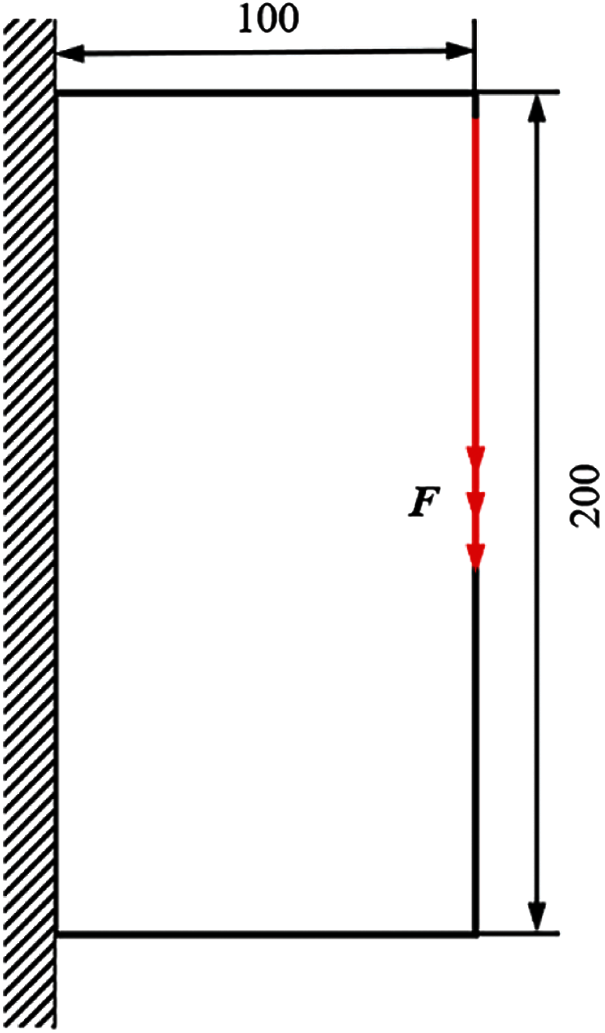
Figure 1: Basic structure for Example 1
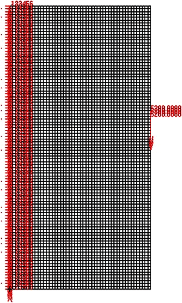
Figure 2: Finite element model for Example 1
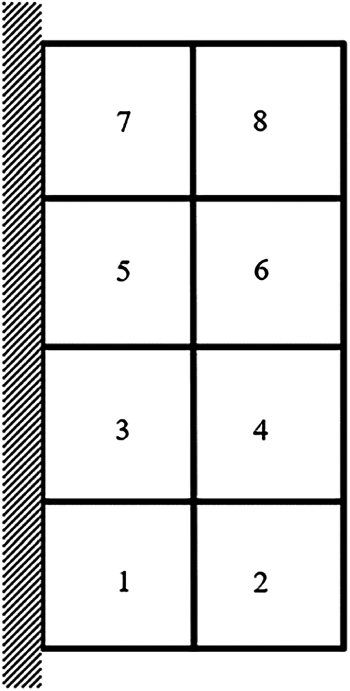
Figure 3: Damage distribution for d = 50
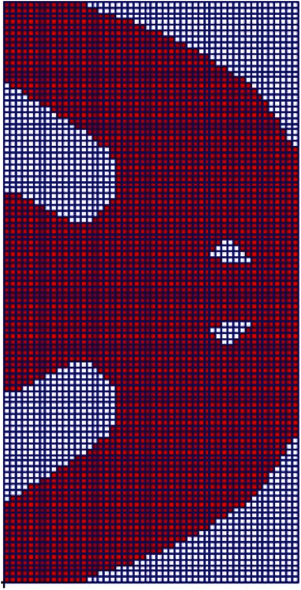
Figure 4: Topology results for Example 1
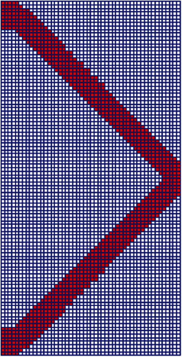
Figure 5: Conventional optimization for Example 1
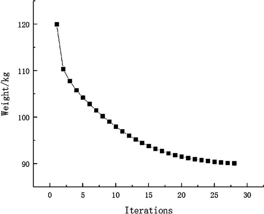
Figure 6: Weight iteration curve for Example 1
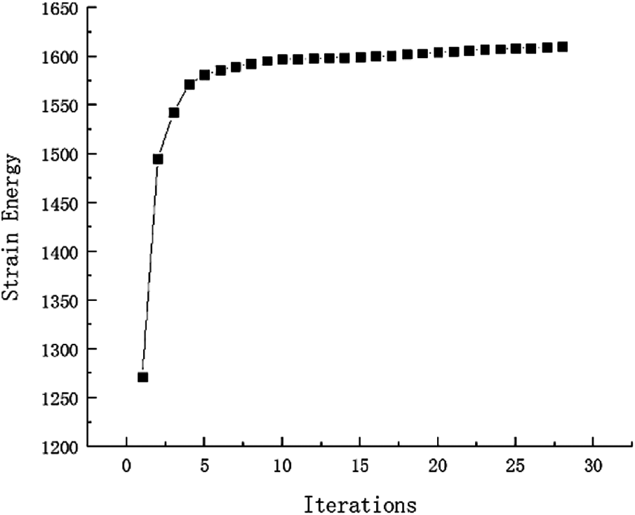
Figure 7: Strain Energy iteration curve for Example 1
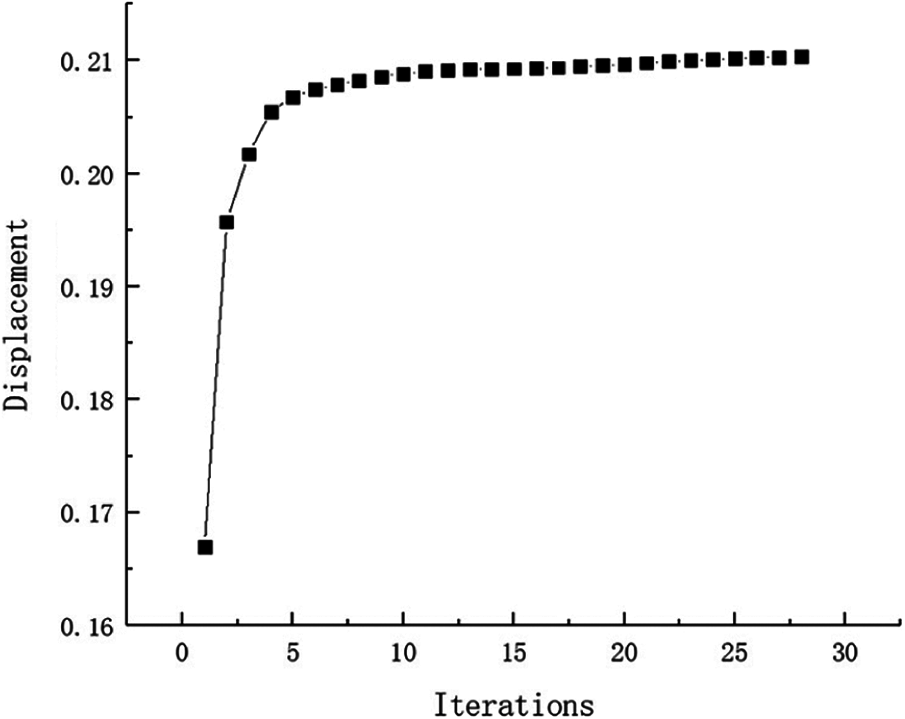
Figure 8: Displacement iteration curve for Example 1
The maximum stress value and maximum displacement value of the structure are obtained in turn after occurring failure on failure regions of optimization structure. Because of the symmetry, the stress and displacement distribution of the optimal topological structure under eight failure working conditions is only indicated by the first four failure working conditions, as shown in Figs. 9 and 10. The following conclusions can be drawn from these stress and displacement distribution diagrams: When local failure occurs, the stress value of some elements close to concentrated force is much larger than the allowable stress, thus this part should be reprocessed by shape optimization. The maximum displacement value generally occurs at the place where the external load is loaded or near failure regions. From comparing with four failure working conditions, it has the greatest effect on the optimization structure when the fourth region damaged. Due to symmetry, the sixth failure region is the worst failure working condition too. These two are failure regions on both sides of concentrated force. Therefore, extra measures may be taken for the optimized structure safety near the loading place in engineering practice.
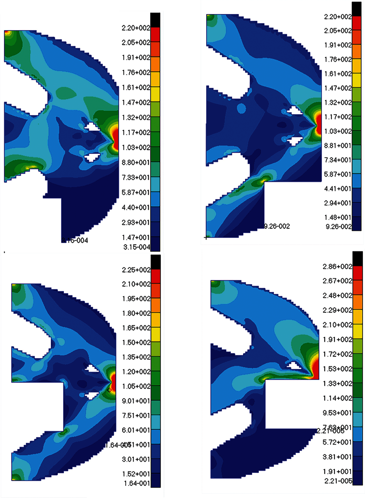
Figure 9: The stress diagrams of optimum structure for Example 1 with four failure working conditions
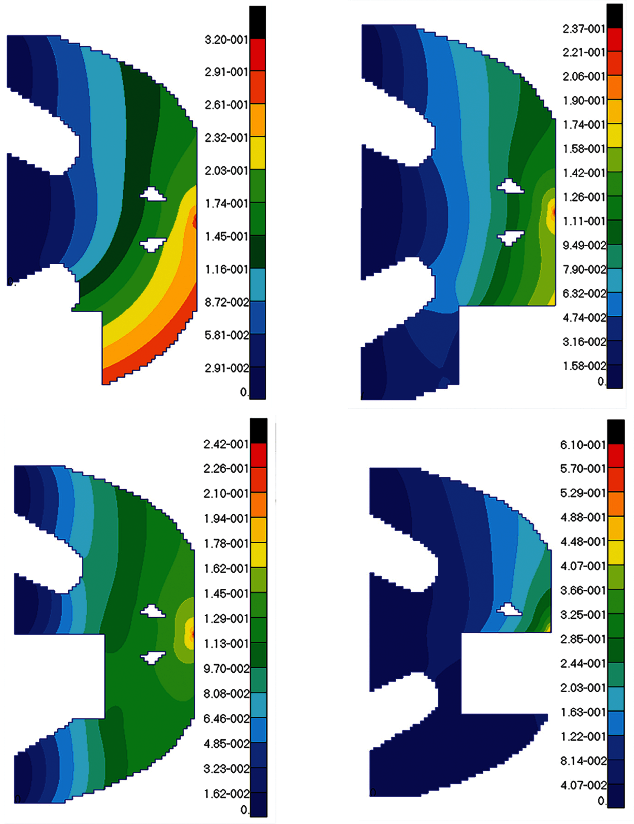
Figure 10: The displacement diagrams of optimum structure for Example 1 with four failure working conditions
Using the single constraint to verify this approach availability. The model is calculated with single constraint as stress. The topology optimization structure obtained is as follows (Fig. 11). And the weight of this optimization is 50.23 kg. It can be seen that weight of objective function structure decreases continuously and reaches the optimal value after iterations from the iterative curve of structure weight optimization Fig. 12. In a similar way, the model with single constraint as displacement is calculated and final result for weight is 88.75 kg. The topology result and weight iteration curve are shown in Figs. 13 and 14. As the constraint is changed, as the optimal topology is changed. This approach for topology calculation is effective.
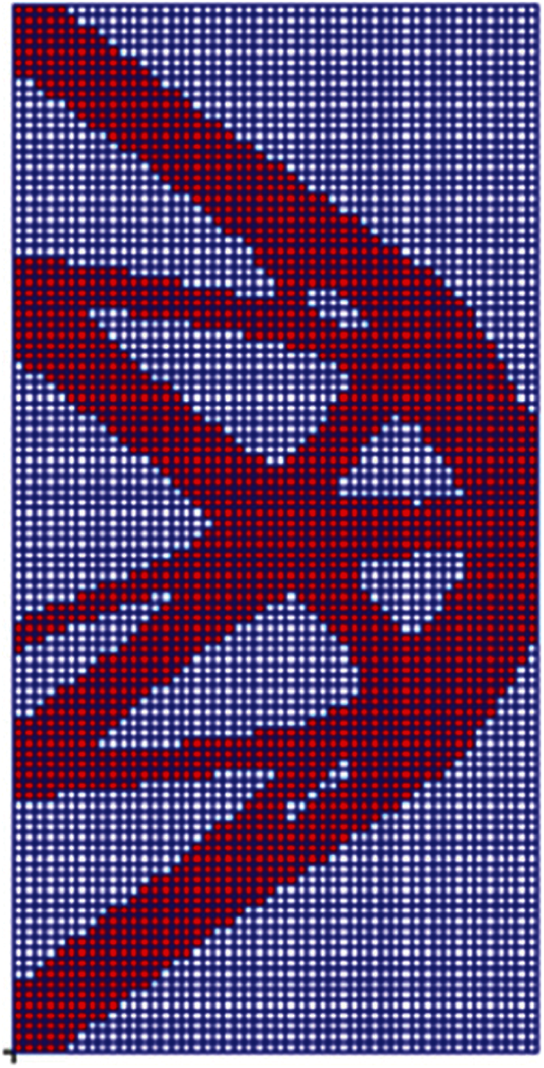
Figure 11: Topology results for stress constraint
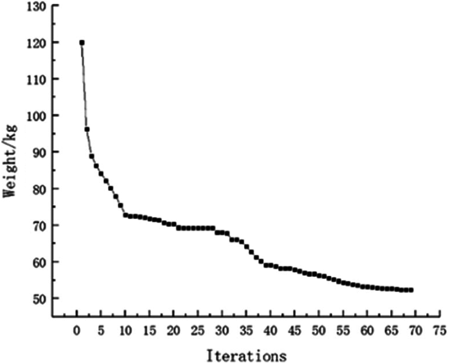
Figure 12: Weight iteration curve for stress constraint
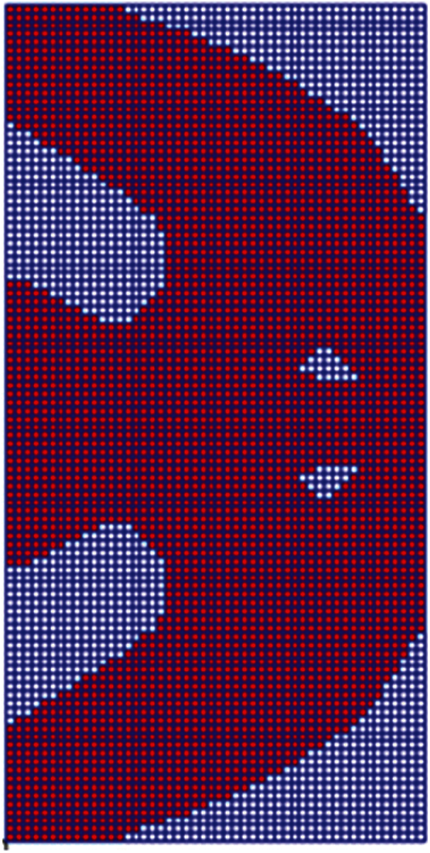
Figure 13: Topology results for displacement constraint
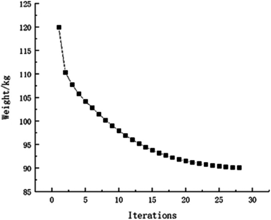
Figure 14: Weight iteration curve for displacement constraint
Example 2: The basic structure is the same as Example 1, and other factors are unchanged. Then considering 32 failure regions, every failure region is a square evenly distributed with side length d = 25 mm as shown in Fig. 15. The inversion threshold is 0.23 and the convergence accuracy is same as the last 0.001. The weight of optimization result is 46.42 kg after 44 iterations and inversion. The weight iteration curve diagram in the optimization process is Fig. 16, and the optimization result is shown in Fig. 17. And that, the change curve of constraints value with iterations is shown in Figs. 18 and 19. As can be seen from the figure, the constraint value increases and tends to be stable as the number of iterations increases.
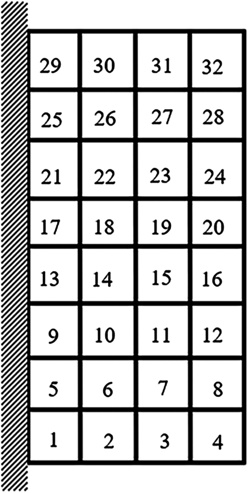
Figure 15: Damage distribution for Example 2
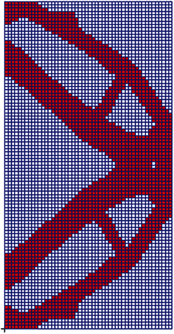
Figure 16: Topology results for Example 2
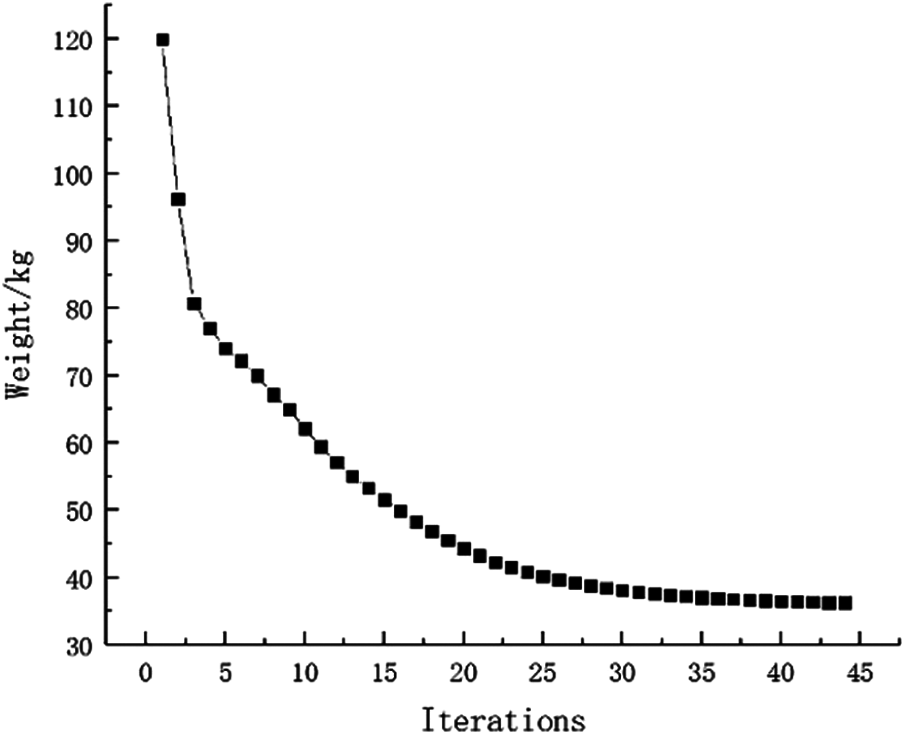
Figure 17: Weight iteration curve for Example 2
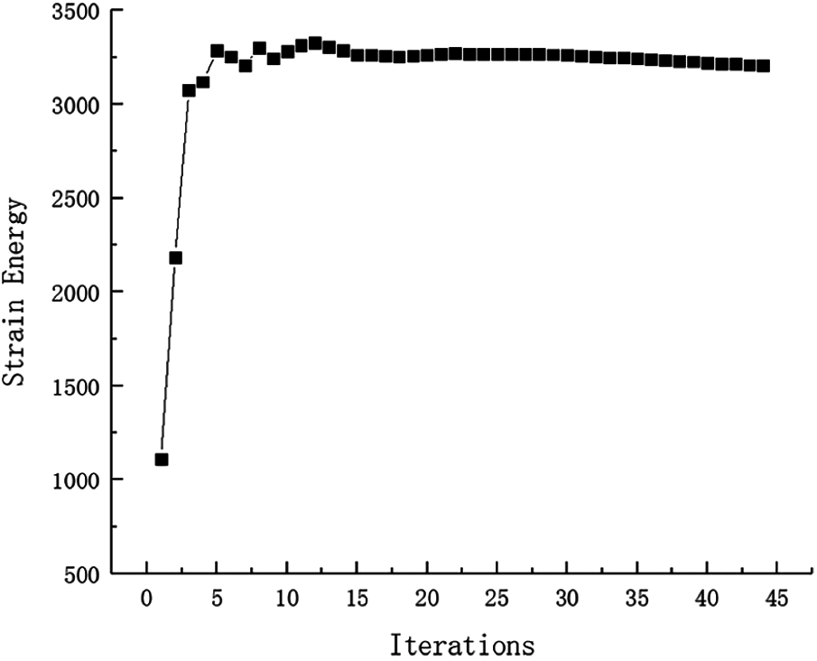
Figure 18: Strain Energy iteration curve for Example 2
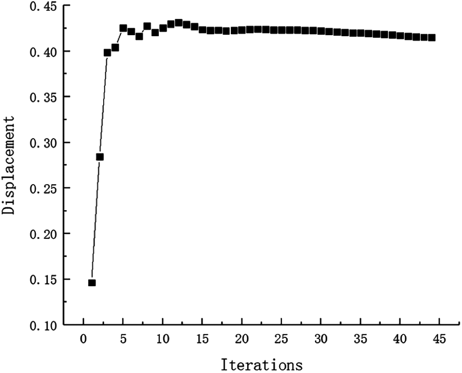
Figure 19: Displacement iteration curve for Example 2
According to comparing the topology optimization structure and its corresponding structure weight (see Figs. 4, 5 and 16), the conclusions are obtained that weight of the optimization structure decreases with the decrease of the failure region’s size. When the size of failure region is 0, namely without considering failure working condition, the optimization structure has the minimum weight, the lowest redundancy and the most sensitive for local failure.
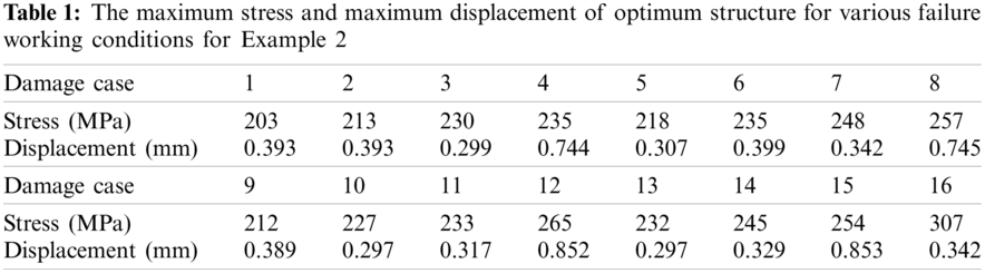
Because of the structure’s symmetry, it is only shown that the maximum stress value and the maximum displacement value in the first 16 failure regions in Tab. 1. It is similar to the Example 1 that the maximum stress values of these failure working conditions are all larger than the allowable stress value, but elements of exceeding part is very few and should be further processed by other way. From the Tab. 1, the ratio of number of elements whose von mises stress and displacement value are under the allowable value is over 99%. After No. 16 and No. 20 failure working conditions occurred, the maximum value increase sharply and the structure is the most sensitive to damage in these two regions comparing with the other failure working conditions.
Example 3: The basic structure is a 120 mm
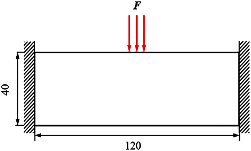
Figure 20: Basic structure for Example 3
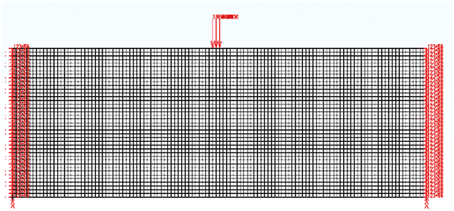
Figure 21: Finite element model for Example 3
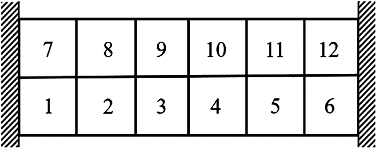
Figure 22: Damage distribution for Example 3
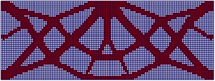
Figure 23: Topology results for Example 3
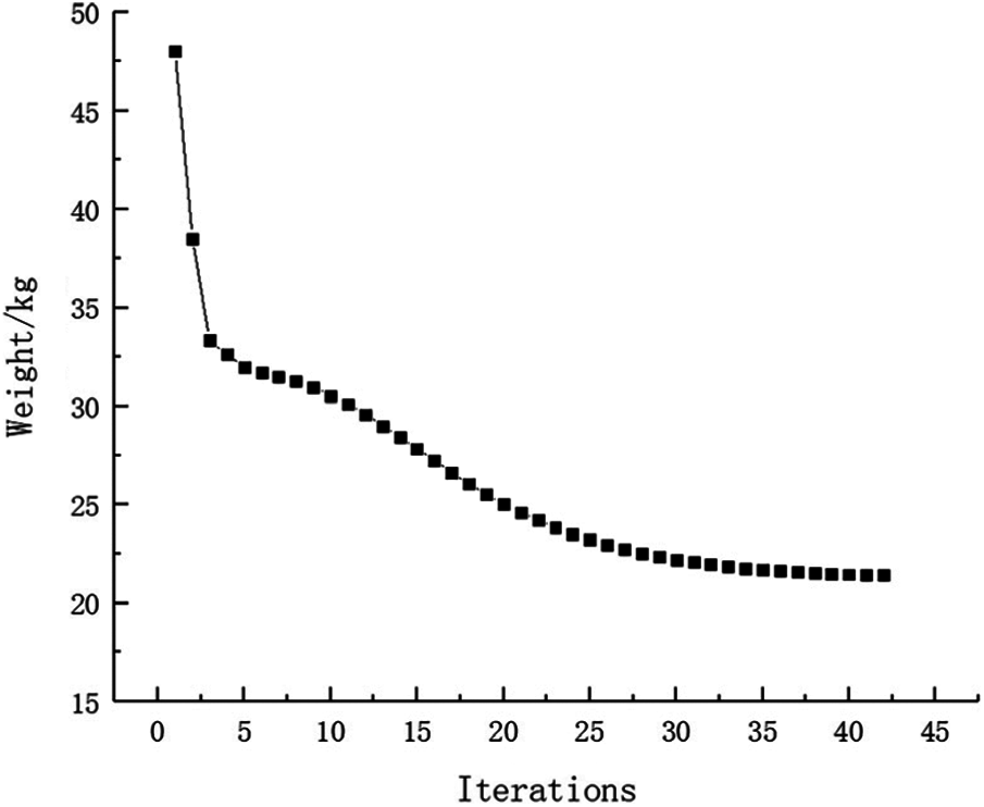
Figure 24: Weight iteration curve for Example 3
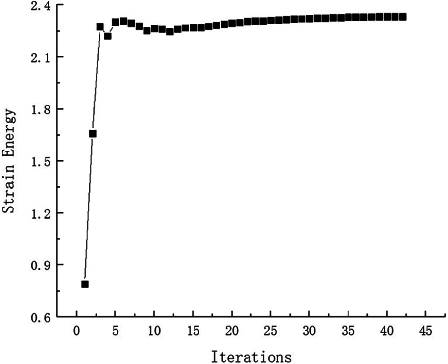
Figure 25: Strain Energy iteration curve for Example 3
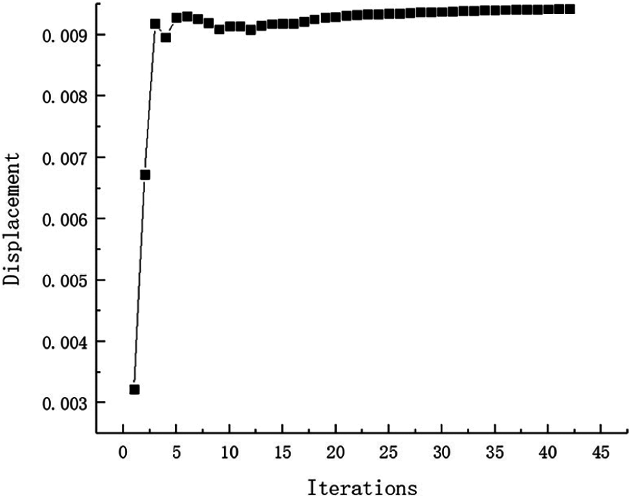
Figure 26: Displacement iteration curve for Example 3
After failure regions damage in turn, the simulation value of the maximum stress and maximum displacement are obtained. Because of symmetry, the stress and displacement distribution of the optimization topologic structure under 12 failure working conditions is only indicated by the left six in left side of central axis. The following conclusions can be drawn from these stress and displacement distribution diagrams in Figs. 27 and 28: The maximum stress generally occurs near force loading, boundary conditions, or around failure regions. The maximum displacement generally occurs at the place where the external load is loaded or near the direction of force vector. When local damage occurs, the stress value of some elements close to concentrated force is much large but still smaller than the allowable stress. when the No. 9 failure region damage, the stress of this part exceeding the allowable stress should be optimized in section.
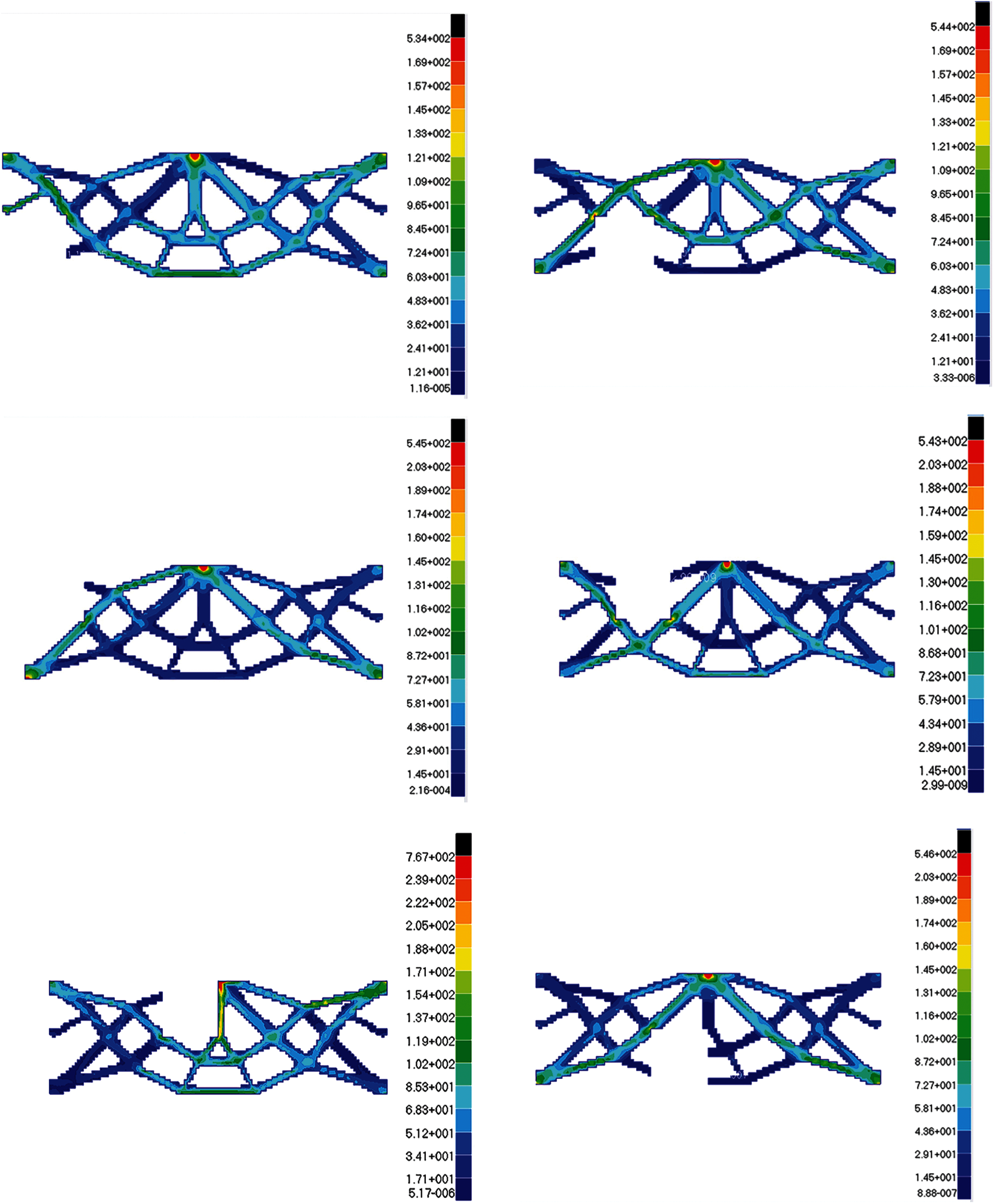
Figure 27: The stress diagrams of optimum structure for Example 3 with six working conditions
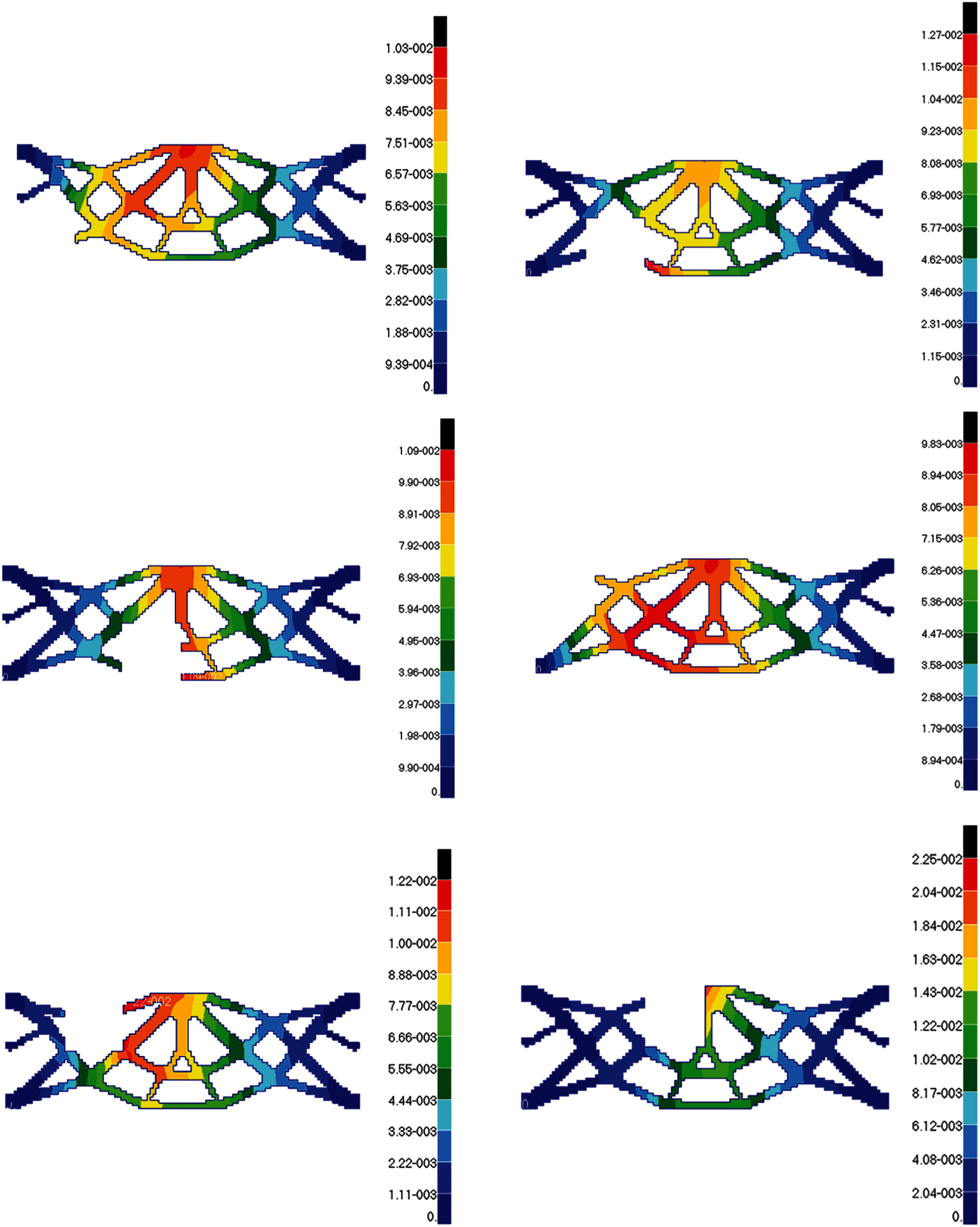
Figure 28: The displacement diagrams of optimum structure for Example 3 with six working conditions
According to comparing with six damage conditions, the No. 9 failure working condition is not only the case where the maximum stress and maximum displacement occurs, but also the most dangerous in all failure working conditions. If the stress or displacement value after local failure is larger, the possibility of structural collapse is greater, so it can be called dangerous working conditions. Due to symmetry, the tenth failure working condition is the worst too. On the contrary, the maximum stress value and displacement value are the minimum in failure working conditions when the No. 7 region damages. In other words, the structure can be optimized more for lightweight and lower cost in the safest No. 7 and No. 12 regions.
Example 4: The basic structure is the same to example 3, and other factors are unchanged. Then considering 48 failure regions, the value of square failure region is 10 mm, evenly distributed in the base structure as shown in Fig. 29. The inversion threshold is 0.71 and the convergence accuracy is same to the last 0.001. The weight of optimization result is 17.32 kg after 44 iterations and inversion, and the optimization result is shown in Fig. 30. The weight iteration curve diagram in the optimization process is Fig. 31. And that, the change curve of constraints value with iterations is shown in Figs. 32 and 33. As can be seen from the figure, the constraint value increases and tends to be stable as the number of iterations increases.
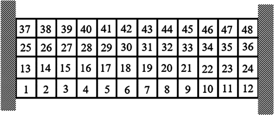
Figure 29: Damage distribution for Example 4
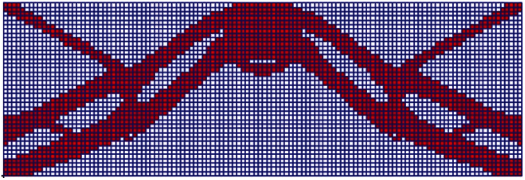
Figure 30: Topology results for Example 4
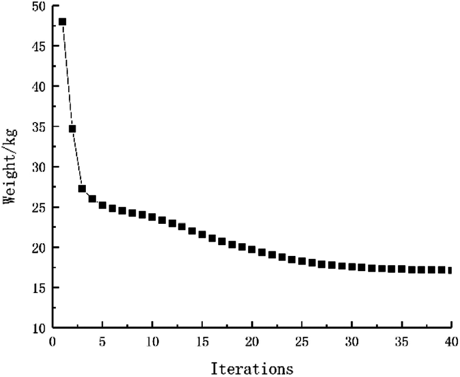
Figure 31: Weight iteration curve for Example 4
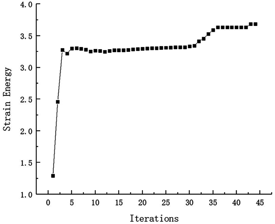
Figure 32: Strain Energy iteration curve for Example 4
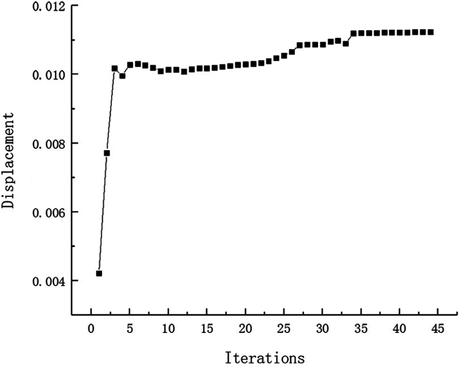
Figure 33: Displacement iteration curve for Example 4
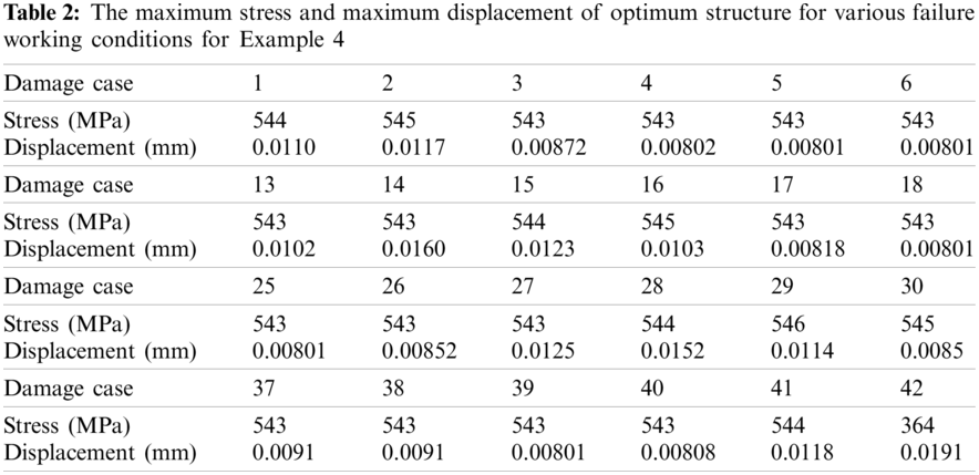
Due to the structure’s symmetry, the left regions are damaged in turn. It is only shown that the maximum stress value and maximum displacement value in Tab. 2. Both the stress value and the displacement value are under the allowable limit when fail occurs. The No. 42 failure working condition is the worst case with the maximum displacement value, so the No. 43 is the worst also. It is different from the previous examples that the maximum stress value of No. 42 failure working condition is not the maximum in all working conditions as speculated but is the minimum in all while the displacement value is almost equal to the allowable value.
Example 5: The basic structure is a well-known L-type beam as shown in Fig. 34. L-type beam is discretized using quad finite elements with the size of 1
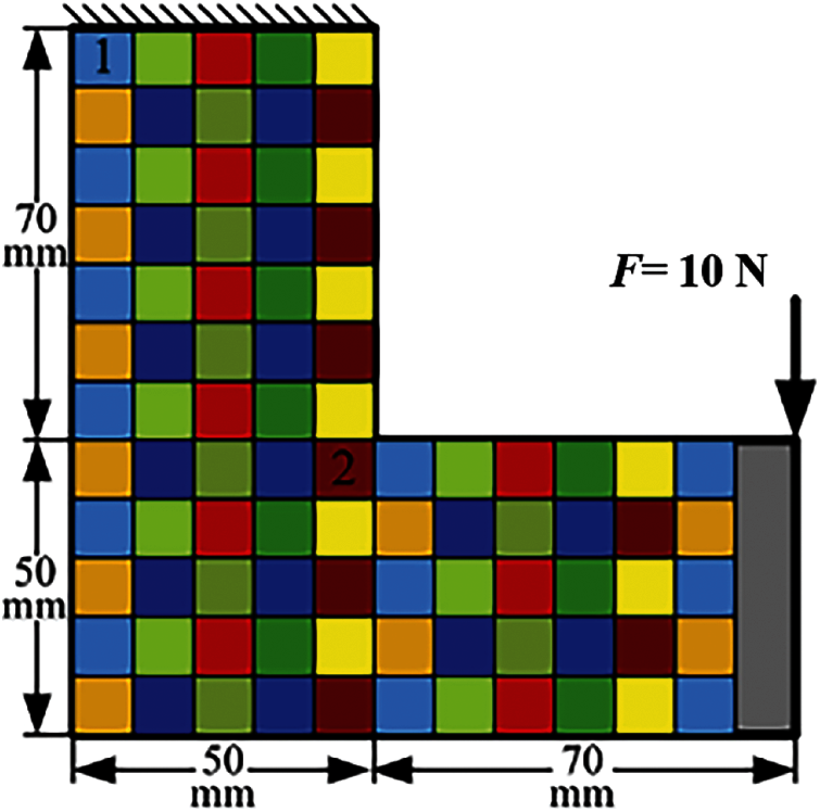
Figure 34: Basic structure and damage distribution
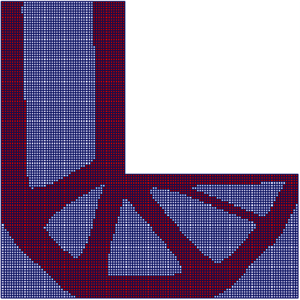
Figure 35: Topology results for Example 5
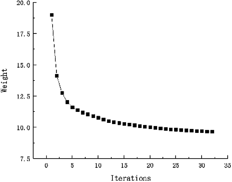
Figure 36: Weight iteration curve for Example 5
And that, the change curve of constraints value with iterations is shown in Figs. 37 and 38. As can be seen from the figure, the constraint value increases and tends to be stable as the number of iterations increases. The maximum value of the displacement and stress in topology result are 0.02007 mm and 158 MPa, they all meet the constraint condition approximatively. Due to many working conditions, it is not enumerated that maximum stress and maximum displacement of optimum structure for various failure working conditions. Both the stress value and the displacement value are under the allowable limit when fail occurs.
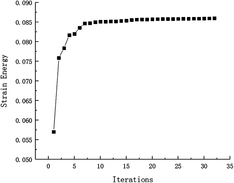
Figure 37: Strain Energy iteration curve for Example 5
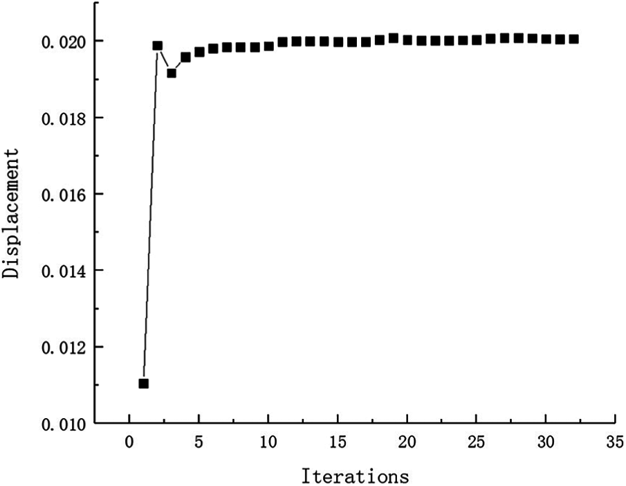
Figure 38: Displacement iteration curve for Example 5
To assess the merit of the proposed fail-safe models than other fail-safe structures. Let compare Example 5 with literature [28] chapter 5.2. Literature [28]’s arithmetic is based on the von mises stress and used the KS function to approximate the max-operator. Fig. 39 is the topology results for literature [28]. Compare two results, both methods meet the design requirements with considering fail-safe working conditions. But the structure configuration obtained by this paper is simpler than other, we can get it is easier to construct in actual engineering construction based this paper method. However, this method computing speed is slower. The direction of the future work will be done to improve the calculation speed and efficiency.
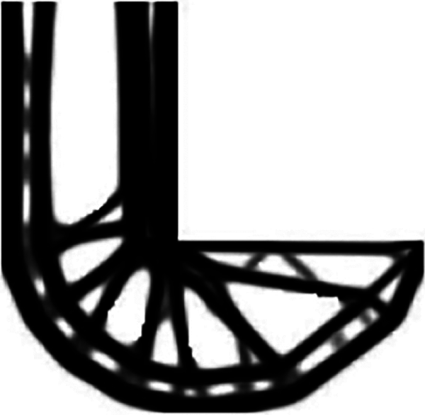
Figure 39: Topology results by literature [28] for Example 5
At present, researchers study fail-safe topology optimization for a certain objective are based on the analysis of a single constraint, whereas the fail-safe optimization model with multiple constrains is very few. The innovation of this paper is about these: this method can increase redundancy obviously by adding more materials, although fail-safe optimized structure looks cumbersome with more weight. The influence of structural strength and stiffness on the design is considered comprehensively in fail-safe topology optimization, and the practical engineering applications are taken into consideration by imposing multiple constraints on the structural performances. Once the local failure occurs, fail-safe optimized structure can still survive normal loading conditions, which is complied with the fail-safe concept.
Based on ICM method, this paper establishes a continuum topology optimization model considering fail-safe condition for weight minimization with constraints on stress and displacement, which is solved efficiently by using DSQP. By means of five examples, it is proved that the fail-safe topology optimization with multiple constraints is valid. Compared with other topology optimization methods, the proposed method has some advantages, such as simple formulations and easy implementation. From the perspective of design logic, the multiple constraints and objective are feasible and effective. In terms of the research in fail-safe topology optimization, the method adopted in this research extends single constraint to multiple constraints, and it provides a good reference for designers with the idea of studying the most dangerous failure region. For practical engineering, the requirements of stress and displacement are both important and indispensable to a design. The optimized designs reveal more practical significance for engineering applications. When the local failure occurs, the optimized structure obtained from fail-safe design can avoid greater economic losses and even human casualties.
Funding Statement: This work showed in this paper has been supported by the National Natural Science Foundation of China (Grant 11872080).
Conflicts of Interest: The authors declare that they have no conflicts of interest to report regarding the present study.
1. Michell, A. G. M. (1904). The limits of economy of materials in frame structures. Philosophical Magazine, 8(47), 589–597. DOI 10.1080/14786440409463229. [Google Scholar] [CrossRef]
2. Guest, J. K. (2009). Imposing maximum length scale in topology optimization. Structural and Multidisciplinary Optimization, 37(5), 463–473. DOI 10.1007/s00158-008-0250-7. [Google Scholar] [CrossRef]
3. Wu, J., Aage, N., Westermann, R., Sigmund, O. (2018). Infill optimization for additive manufacturing-approaching bone-like porous structures. IEEE Transactions on Visualization and Computer Graphics, 24(2), 1127–1140. DOI 10.1109/TVCG.2017.2655523. [Google Scholar] [CrossRef]
4. Huang, G. M., Yang, H. L., Liu, M. M., Ge, S. L., He, Q. L. (2018). Structural optimization design of a certain aircraft gun closed bearing band sabot based on variable density method. Journal of Physics: Conference Series, 1087(4), 62–62. DOI 10.1088/1742-6596/1087/4/042062. [Google Scholar] [CrossRef]
5. Grégoire, A., Perle, G., Olivier, P. (2019). Topology optimization of modulated and oriented periodic microstructures by the homogenization method. Computers and Mathematics with Applications, 78(7), 2197–2229. DOI 10.1016/j.camwa.2018.08.007. [Google Scholar] [CrossRef]
6. Sui, Y. K., Peng, X. R. (2018). Modeling, solving and application for topology optimization of continuum structures. Beijing: Tsinghua university press. [Google Scholar]
7. Pasi, T. (2002). The evolutionary structural optimization method: Theoretical aspects. Computer Methods in Applied Mechanics and Engineering, 191(47), 5485–5498. DOI 10.1016/S0045-7825(02)00464-4. [Google Scholar] [CrossRef]
8. Zhang, W. S., Yuan, J., Zhang, J., Guo, X. (2016). A new topology optimization approach based on moving morphable components (MMC) and the ersatz material model. Structural and Multidisciplinary Optimization, 53(6), 1243–1260. DOI 10.1007/s00158-015-1372-3. [Google Scholar] [CrossRef]
9. Yuan, S. (1988). The theory of structural redundancy and its effect on structural design. Computers & Structures, 28(1), 15–24. DOI 10.1016/0045-7949(88)90087-9. [Google Scholar] [CrossRef]
10. Peng, X. R., Sui, Y. K. (2018). ICM method for fail-safe topology optimization of continuum structures. Chinese Journal of Theoretical and Applied Mechanics, 50(3), 611–621. DOI 10.6052/0459-1879-17-366. [Google Scholar] [CrossRef]
11. Nguyen, D. T., Arora, J. S. (1982). Fail-safe optimal design of complex structures with substructures. Journal of Mechanical Design, 104(4), 861–868. DOI 10.1115/1.3256449. [Google Scholar] [CrossRef]
12. Bendsøe, M. P., Dıaz, A. R. (1998). A method for treating damage related criteriain optimal topology design of continuum structures. Structural and Multidisciplinary Optimization, 16(2–3), 108–115. DOI 10.1007/BF01202821. [Google Scholar] [CrossRef]
13. Jansen, M., Lombaert, G., Schevenels, M., Sigmund, O. (2014). Topology optimization of fail-safe structures using a simplified local damage model. Structural & Multidisciplinary Optimization, 49(4), 657–666. DOI 10.1007/s00158-013-1001-y. [Google Scholar] [CrossRef]
14. Zhou, M., Fleury, R. (2016). Fail-safe topology optimization. Structural and Multidisciplinary Optimization, 54(5), 1225–1243. DOI 10.1007/s00158-016-1507-1. [Google Scholar] [CrossRef]
15. Du, J. Z., Guo, Y. H., Chen, Z. M., Sui, Y. K. (2019). Topology optimization of continuum structures considering damage based on independent continuous mapping method. Acta Mechanica Sinica, 35(2), 433–444. DOI 10.1007/s10409-018-0807-7. [Google Scholar] [CrossRef]
16. Du, J. Z., Meng, F. W., Guo, Y. H., Sui, Y. K. (2020). Fail-safe topology optimization of continuum structures with fundamental frequency constraints based on the ICM method. Acta Mechanica Sinica, 36(5), 1–13. DOI 10.1007/s10409-020-00988-7. [Google Scholar] [CrossRef]
17. Long, K., Wang, X., Du, Y. X. (2019). Robust topology optimization formulation including local failure and load uncertainty using sequential quadratic programming. International Journal of Mechanics and Materials in Design, 15(2), 317–332. DOI 10.1007/s10999-018-9411-z. [Google Scholar] [CrossRef]
18. Lüdeker, J. K., Benedikt, K., (2019). Fail-safe optimization of beam structures. Journal of Computational Design and Engineering, 6(3), 260–268. DOI 10.1016/j.jcde.2019.01.004. [Google Scholar] [CrossRef]
19. Li, Z. S., Gao, X. L., Tang, Z. C. (2020). Safety performance of a precast concrete barrier: Numerical study. Computer Modeling in Engineering & Sciences, 123(3), 1105–1129. DOI 10.32604/cmes.2020.09047. [Google Scholar] [CrossRef]
20. Ambrozkiewicz, O., Kriegesmann, B. (2020). Density-based shape optimization for fail-safe design. Journal of Computational Design and Engineering, 7, 1–15. DOI 10.1093/jcde/qwaa044. [Google Scholar] [CrossRef]
21. Zhao, G., Yang, J. M., Wang, W., Zhang, Y., Du, X. X. et al. (2020). T-splines based isogeometric topology optimization with arbitrarily shaped design domains. Computer Modeling in Engineering & Sciences, 123(3), 1033–1059. DOI 10.32604/cmes.2020.09920. [Google Scholar] [CrossRef]
22. Chen, Z., Long, K., Wen, P., Nouman, S. (2020). Fatigue-resistance topology optimization of continuum structure by penalizing the cumulative fatigue damage. Advances in Engineering Software, 150. 102924–102924. DOI 10.1016/j.advengsoft.2020.102924. [Google Scholar] [CrossRef]
23. Dou, S. G., Mathias, S. (2021). On stress-constrained fail-safe structural optimization considering partial damage. Structural and Multidisciplinary Optimization, 63(5), 929–933. DOI 10.1007/S00158-020-02782-2. [Google Scholar] [CrossRef]
24. Cheng, G. D., Zhang, D. X. (1995). Topology optimization of stress-constrained planar elastomer. Journal of Dalian University of Technology (Social Sciences), 35(1), 1–9. DOI CNKI:SUN:DLLG.0.1995-01-000. [Google Scholar]
25. Sui, Y. K., Zhang, X. S., Long, L. C. (2007). ICM method of the topology optimization for continuum structures with stress constraints approached by the integration of strain energies. Chinese Journal of Computational Mechanics, 24(5), 602–608. DOI CNKI:SUN:JSJG.0.2007-05-013. [Google Scholar]
26. Alexander, V., Matthijs, L., Fred, V. K. (2017). A unified aggregation and relaxation approach for stress-constrained topology optimization. Structural and Multidisciplinary Optimization, 55(2), 663–679. DOI 10.1007/s00158-016-1524-0. [Google Scholar] [CrossRef]
27. Chu, S., Xiao, M., Gao, L., Li, H. (2019). A level set–based method for stress-constrained multimaterial topology optimization of minimizing a global measure of stress. International Journal for Numerical Methods in Engineering, 117(7), 800–818. DOI 10.1002/nme.5979. [Google Scholar] [CrossRef]
28. Wang, H. X., Liu, J., Wen, G. l., Xie, Y. M. (2020). The robust fail-safe topological designs based on the von mises stress. Finite Elements in Analysis and Design, 171(C), 103376–103376. DOI 10.1016/j.finel.2019.103376. [Google Scholar] [CrossRef]
29. Meng, Q. X., Xu, B., Wang, C., Zhao, L. (2020). Stress constrained thermo-elastic topology optimization based on stabilizing control schemes. Journal of Thermal Stresses, 43(8), 1040–1068. DOI 10.1080/01495739.2020.1766391. [Google Scholar] [CrossRef]
30. Simonetti, H. L., Neves, F. A., Almeida, V. S. (2021). Multi objective topology optimization with stress and strain energy criteria using the SESO method and a multicriteria tournament decision. Structures, 30, 188–197. DOI 10.1016/j.istruc.2021.01.002. [Google Scholar] [CrossRef]
31. Sui, Y. K., Zhang, X. S., Long, L. C. (2006). Topology optimization of continuum structures with the integrated approach of displacement constraints. Acta Mechanica Solida Sinica, 27(1), 102–107. DOI 10.19636/j.cnki.cjsm42-1250/o3.2006.01.018. [Google Scholar] [CrossRef]
32. Xie, Y. J., Rong, J. H., Yu, L. H., Zhu, H. F., Li, F. Y. (2017). Evolutionary structural topology optimization designs with multiple displacement constraints. Modern Manufacturing Engineering, (819–28. DOI 10.16731/j.cnki.1671-3133.2017.08.004. [Google Scholar] [CrossRef]
33. Zhu, R., Sui, Y. K. (2012). Topology optimization of plate-and shell-like structures with displacement constraints under multi-state loadings based on ICM method. Chinese Journal of Solid Mechanics, 33(1), 81–90. DOI 10.19636/j.cnki.cjsm42-1250/o3.2012.01.012. [Google Scholar] [CrossRef]
34. Long, K., Chen, Z., Gu, C. L., Wang, X. (2020). Structural topology optimization method with maximum displacement constraint on load-bearing surface. Acta Aeronautica et Astronautica Sinica, 41(7), 192–199. DOI 10.7527/S1000-6893.2019.23577. [Google Scholar] [CrossRef]
35. Peng, X., Sui, Y. K. (2019). Parameter effect analysis of local failure modes for fail-safe topology optimization. Chinese Journal of Computational Mechanics, 3(4), 317–323. DOI CNKI:SUN:JSJG.0.2019-03-004. [Google Scholar]
 | This work is licensed under a Creative Commons Attribution 4.0 International License, which permits unrestricted use, distribution, and reproduction in any medium, provided the original work is properly cited. |