Investigation on the Indeterminate Information of Rock Joint Roughness through a Neutrosophic Number Approach

Changshuo Wang; Liangqing Wang; Shigui Du; Jun Ye; Rui Yong

doi:10.32604/cmes.2021.017453

1Institute of Rock Mechanics, Ningbo University, Ningbo, 315211, China
2Faculty of Engineering, China University of Geosciences, Wuhan, 430074, China
3Department of Civil Engineering, Shaoxing University, Shaoxing, 312000, China
*Corresponding Author: Liangqing Wang. Email: wangliangqing@cug.edu.cn
Received: 11 May 2021; Accepted: 13 July 2021

Abstract: To better estimate the rock joint shear strength, accurately determining the rock joint roughness coefficient (JRC) is the first step faced by researchers and engineers. However, there are incomplete, imprecise, and indeterminate problems during the process of calculating the JRC. This paper proposed to investigate the indeterminate information of rock joint roughness through a neutrosophic number approach and, based on this information, reported a method to capture the incomplete, uncertain, and imprecise information of the JRC in uncertain environments. The uncertainties in the JRC determination were investigated by the regression correlations based on commonly used statistical parameters, which demonstrated the drawbacks of traditional JRC regression correlations in handling the indeterminate information of the JRC. Moreover, the commonly used statistical parameters cannot reflect the roughness contribution differences of the asperities with various scales, which induces additional indeterminate information. A method based on the neutrosophic number (NN) and spectral analysis was proposed to capture the indeterminate information of the JRC. The proposed method was then applied to determine the JRC values for sandstone joint samples collected from a rock landslide. The comparison between the JRC results obtained by the proposed method and experimental results validated the effectiveness of the NN. Additionally, comparisons made between the spectral analysis and common statistical parameters based on the NN also demonstrated the advantage of spectral analysis. Thus, the NN and spectral analysis combined can effectively handle the indeterminate information in the rock joint roughness.

Keywords: Rock joint roughness coefficient; uncertainty; indeterminate information; neutrosophic number; spectral analysis

Many major foundation projects have been constructed in complex geological conditions, and numerous high rock slopes are formed. The rock joints in the rock slopes are affected by the geological forces inside and outside the earth, making the slope easy to slip along the controlled joints [1,2]. Thus, the rock joint shear strength is crucial in determining the stability of rock slopes. To better estimate the rock joint shear strength, accurately determining the rock joint roughness is the first step faced by researchers and engineers [3–5].

The joint roughness coefficient (JRC) proposed by Muralha et al. [6] is closely related to the rock joint shear strength and is widely used in engineering practice. Its value is commonly obtained by visual judgment based on the proposed standard profiles [6]. Considering subjectivity exists in the visual comparison process determining the JRC, many quantitative approaches, i.e., experimental [7,8], statistical [4,9–11], and fractal methods [12–14] have been proposed to determine the JRC objectively. Although these regression equations between JRC and roughness parameters have high correlation coefficients, there are still deviations in the JRC calculation results [15]. Two main reasons contributed to the calculation deviation. First, the mechanical properties of geological bodies contain much indeterminate information [16]. It is difficult to provide exact JRC values in these cases. In addition, there are nonuniformity, anisotropy, inhomogeneity, and scale effects on the rock joint roughness [17]. Second, the rock joint profile consists of low and high-frequency asperities [18,19]. The commonly used roughness parameters have a deficiency in capturing those kinds of asperities, which results in bias description of joint roughness [18]. Due to the above two limitations, finding a certain equation for accurately determining the JRC based on the traditional approach is not easy.

Considering the contribution of different frequency components of the rock joint surface to the roughness are generally different, Wang et al. [18] derived a spectral roughness parameter to determine the JRC. This spectral roughness parameter considers the contribution differences among various scales of asperity components. However, the spectral analysis can only provide determinate expressions of the JRC but cannot express the indeterminate information of the JRC data. Due to the incompleteness of observations and measurements, it is necessary to approximate the JRC in indeterminate environments. Neutrosophy puts forward the concepts between true and false: neutral, indeterminate, incomplete, etc. The neutrosophic number (NN) concept was first introduced by Smarandache et al. [20–22], which has been proved to express determinate and indeterminate information. Thus, the combination of the NN [20–22] and spectral analysis [18] may overcome the limitations in determining the joint roughness mentioned above.

The NN and other neutrosophic theories such as neutrosophic statistics, neutrosophic probability, and neutrosophic distribution are major branches of the neutrosophic theory, which deals with indeterminate data and indeterminate inference methods that contain degrees of indeterminacy as well [23–25]. Many researchers have contributed to developing the neutrosophic theory in recent years [16,23,24,26,27]. Karamaşa et al. [28] developed a new multi-criteria decision-making method and ranked factors affecting outsourcing-related third-party logistics using neutrosophic AHP. Aslam et al. [29] introduced the student t-test and F-test under neutrosophic statistics to address the drawbacks of classical statistics. Ye et al. [16] established JRC and the shear strength neutrosophic functions based on neutrosophic theory. Later on, Ye et al. [27] adopted neutrosophic number functions to study the anisotropy and scale effect for the indeterminate JRC. Then, Chen et al. [26] proposed neutrosophic interval statistical numbers to express JRC under indeterminate environments. To utilize the current and previous data information, Aslam [30] presented a new approach to determine roughness coefficient neutrosophic numbers based on the neutrosophic exponentially weighted moving average. Du et al. [31] originally expressed the mixed information of the simplified neutrosophic set and NN based on a simplified neutrosophic indeterminate set. Additionally, Du et al. [24] proposed a multi-attribute decision-making approach based on subtraction operational aggregation operators of simplified neutrosophic numbers. However, NN functions applied in the JRC determination mainly focus on the scale effect and anisotropy properties; they have not been applied to determine the JRC for a specific rock joint based on detailed spectral analysis. Hence, this original study will discuss the uncertainties in the existing JRC determination correlations and propose NN functions of determinate and indeterminate JRC based on the spectral analysis. This new approach to determine JRC can consider the contribution of various scale asperity components in determining the rock joint roughness and approximate indeterminate expressions of the JRC.

The structure of this paper is listed as follows. In Section 2, the basic concepts for neutrosophic number functions and spectral analysis are presented. Then, in Section 3, the uncertainties in joint roughness coefficient determination are first discussed. A new method to calculate the JRC based on neutrosophic number functions and spectral analysis is then proposed. In Section 4, the comparisons between the new approach and commonly used statistical parameters to determine the JRC are carried out based on experimental results of the rock joints collected from an actual rock landslides area. Finally, the conclusion is presented in Section 5.

where a and b are real numbers, and I denotes the indeterminate information, and I ∈ [IL, IU]. The indeterminate range I ∈ [IL, IU] can be statistically specified to satisfy practice requirements. In this equation, a and bI are the determinate and indeterminate parts, respectively. Moreover, the NN Z will degenerate to the real number a if b equals zero, which contains only the determinate information. It will degenerate to a NN bI without a determinate part if a equals zero, containing only the indeterminate information.

For example, let us assume that a NN is z = 2 + 4I, where I ∈ [0, 0.2]. Thus, its determinate part is 2, and its indeterminate part is 4I. Then, there is z ∈ [2, 2.8] for I ∈ [0, 0.2].

Generally, the rock joints in engineering practice consist of various scales of asperities. The asperities with small inclinations but high amplitudes are low-frequency components, while the asperities with big inclinations but low amplitudes are high-frequency components. Due to the different frequencies, the various scales of asperity components have different influences on the rock joint shear behavior. To quantitively describe the contribution of asperities with various frequencies on the rock joint roughness, Wang et al. [18] proposed to adopt the spectral analysis method to determine the JRC.

Although the rock joint morphology in engineering practice is so complex that difficult to be described by clear math equations, the spectral characteristics of the profile are readily analyzed by the power spectral density (PSD) [18]. With the help of PSD, the amplitude distribution for the joint profile can be effectively presented in the frequency domain. In this paper, the periodogram method is used to obtain the PSD for a rock joint profile. Herein, the periodogram method estimates the PSD by dividing the square of the joint profile Fourier transform modulus by its sampling length. The detailed information about the spectral analysis on a rock joint profile can be seen in the reference [18], and the calculation method is briefly described as follows.

To simplify the calculation, the least-square fitting line of a rock joint profile is first aligned to be horizontal, and the average straight line of the profile is shifted to coincide with the coordinate axis x. After alignment, the profile can be presented as:

where y(x) is the translated profile; yo(x) is the aligned profile, that the least square fitting line of the profile is horizontal; L is the projection length of the profile on the x-axis.

The average power and Fourier transform of the aligned profile y(x) in the spatial frequency domain are respectively shown as:

where P2D is the average power of y(x); Y(f) is the Fourier transform of y(x) in the spatial frequency domain; f is the spatial frequency of the harmonic components of y(x), and its unit is the reciprocal of length unit of the profile.

where PSD(f) is the power spectral density of the profile; fmin and fmax are the minimum and maximum frequencies of harmonic components, respectively. Note that the negative frequency range of the PSD has no physical meaning in actual engineering practice. From the aspect of energy conservation, the PSD of the negative frequency range can be superimposed on the corresponding positive range to obtain the single-sided power spectral density (PSD*) as:

As indicated by Eqs. (5) and (7), the relation between P2D and PSD can be obtained as:

Eq. (8) indicated that the average power of the profile (i.e., the mean square value of amplitude heights of a rock joint profile) equals to the area enclosed by the PSD* of the profile and the frequency axis. Thus, it is possible to quantitatively analyze the amplitude and height of the joint profile in a certain frequency range.

As the rock joint profile data collected in the engineering practice is discrete under a certain sampling interval, the discrete form of the PSD is presented as follows to facilitate practical applications.

where Ts is the sampling interval; N is the number of discrete points; y(n) is the discrete form of y(x); fm is the discrete form of the harmonic frequency f; k is a positive integer.

Among the various quantitative JRC determination methods, the statistical and fractal methods are widely adopted by researchers and engineers. However, the joint profile in engineering practice is self-affine; different users may get contradictory results with the fractal method [13]. The statistical parameters can be presented by consistent mathematical formulas and can be readily calculated with the help of computer programs; therefore, it is a convenient way to use statistical parameters to determine JRC. The commonly used statistical parameters are average relative height (Rave), maximum relative height (Rmax), standard deviation of height (SDh), average inclination angle (iave), the standard deviation of inclination angle (SDi), root mean square of the first deviation of the profile (Z2), roughness profile index (Rp), structure-function of the profile (SF) and so on [9,11,13,18,33–36]. The detailed calculation formulations of eight statistical parameters can be seen in Tab. 1.

Researchers have been working on statistical parameters to determine the JRC quantitatively, and many regression correlations with high correlation coefficients have been proposed. However, existing regression correlations can only address the determinate information of JRC but cannot express and handle the indeterminate information. Therefore, there may exist deviations in the JRC calculation results for rock joints. To demonstrate the deviations arise from ignoring the incomplete, uncertain, and imprecise information in the JRC, two JRC regression relations based on the widely used statistical parameters Z2 and SF proposed by Li et al. [33] with a 0.4 mm sampling interval were adopted to calculate the JRC. The correlation coefficients for the two regression relations based Z2 and SF are 0.8760 and 0.8725, respectively. The formulas are listes as follows:

The ten standard profiles [8] shown in Fig. 1 are commonly used visual references to determine the JRC in engineering practice. First, the statistical parameters Z2 and SF for the ten standard rock joint profiles were obtained. Then, the JRC values of the standard profiles were calculated according to Eqs. (11), (12). The calculated results and true values of JRC for the standard profiles were both presented in Tab. 2. As shown in Tab. 2, although the correlation coefficients for the above two regression relations are high to 0.8760 and 0.8725, respectively, there are still significant deviations in calculated JRC values. Particularly, the absolute deviations are larger than 70% for the profiles with true JRC values 0.4 and 2.8. Thus, neither the determinate/crisp JRC values based on SF nor Z2 can approximate the roughness of standard rock joint profiles very well. Additionally, the deviations can also be found within other JRC regression correlations based on statistical parameters.

According to the spectral information presented by the rock joint profiles, Wang et al. [18] derived a spectral roughness parameter, PZ. The inclination angle and the amplitude height of rock joints as well as the shear direction can be considered by this spectral joint roughness parameter. Additionally, the contribution differences on joint roughness of various scales of asperities can also be presented. The formulation of the parameter PZ is listed as follows:

Z2∗=[1N∗∑n=0n=N−2(max(0,yn+1−yn)(xn+1−xn)2+(yn+1−yn)2)2]1/2=[1N∗∑n=0n=N∗−1sin2i∗]1/2 (14)

where Pf is an average power index; Z2* is the modified root mean square of the first deviation of the profile; N* is the number of asperities of the rock joint profile facing the shear direction; i* is the inclination angle of asperities of the rock joint profile facing the shear direction; Am is the average power from the frequency fm to fm + 1; Pm is the value of the PSD* corresponding to fm; fmave is the average frequency.

In the study [18], the PZ values were obtained from 112 rock joint profiles digitized by Li et al. [33] at a sampling interval of 0.4 mm, and the correlations between JRC and the roughness parameter PZ were established. The detailed procedure to establish the correlations can be seen in the reference [18].

As suggested by the authors [18], the mean trend correlation JRCmean between the JRC and PZ can be used to predict JRC values. However, as shown in Fig. 2, the JRC values have significant variabilities around the mean trend correlation. Thus, the JRC values determined by the parameter PZ have certain deviations, and the obtained regression correlations can only provide the determinate information of JRC. It cannot express and handle the indeterminate information of JRC. Thus, according to the concept of NNs and the limits of the JRC, the PZ-based NN function for JRC can be written as:

where a1 and a2 are the fitting parameters of the lower limit; b1 and b2 are the differences between the upper bound and lower bound; I is the indeterminacy. In this NN function, a1 + a2 ln PZ and (b1 + b2 ln PZ) I are the determinate and indeterminate parts, respectively.

Figure 2: Correlations between the JRC and PZ at a sampling interval of 0.4 mm [13]

According to Fig. 2, a1 and a2 are 35.80 and 4.84, respectively. The indeterminacy I is set to the interval [0, 0.5] through the statistical analysis of all collected rock joint profiles. Thus, b1 and b2 are twice the differences between the upper bound and lower bound. Obviously, b1 is 9.6, and b2 is 0. Then, the PZ-based NN function for the JRC can be presented as:

The PZ-based NN function expressed in Eq. (19) has two advantages: (1) the spectral roughness parameter PZ is adopted to capture the rock joint profile spectral characteristics, which can effectively reflect the contribution of various scales of asperity components of joint profiles in determing the JRC; (2) the NN function for JRC can determine the JRC in indeterminate environments, which are very suitable to determine the JRC with vague, incomplete, imprecise, and indeterminate information.

Five well-matched sandstone joint samples were collected from the Majiagou landslide. The Majiagou landslide is in Guizhou Town, Zigui County, Yichang City, Hubei Province, China. It is located at the foot of Woniu Mountain on the left bank of the Yangtze River, on the left bank of the Zhaxi River, a tributary of the Yangtze River, and 2.1 km from the mouth of the Yangtze River. The bedrock stratum in the landslide area is the Upper Jurassic Suining Formation (J3S), which belongs to the middle of the Guizhou Group. The lithology is mainly gray-white feldspar quartz sandstone and fine sandstone, with purple-red silty mudstone and mudstone. The sandstone joint samples collected in this paper are mainly gray-white feldspar quartz sandstone joints.

These collected five well-matched sandstone joint samples were cut into standard samples with a length and width of 10 cm and height of 5 cm. Then, a laser scanner was used to scan the surface of these samples with an accuracy of ±35 μm and a sampling interval of 0.2 mm. A photograph of the laser scanner and data acquisition system can be seen in Fig. 3. After the scanning tests, these samples were encapsulated into blocks of cement and cured for 21 days. Finally, these joint samples were subjected to direct shear tests under constant normal stresses. Particularly, the shear velocity was set as 0.4 mm/min, which is consistent with the ISRM suggestions [6]. The direct shear test results for these sandstone joint samples are presented in Tab. 2. In addition, Schmidt hammer rebound tests and direct shear tests performed on planar joint samples were conducted, from which the obtained JCS is 45.9 MPa, and the obtained φb is 26.8°. Then, the true JRC values for the collected sandstone joint samples were back-calculated from the JRC-JCS model [8] and tabulated in Tab. 3.

The 3D surfaces of the collected five sandstone joints were also constructed with the same sampling interval (i.e., 0.4 mm), which is consistent with the PZ-based NN function for JRC determination. Since the samples had been placed parallel to the direct shear plane, these three-dimensional (3D) surfaces were also aligned by setting their corresponding least-square planes to be horizontal, consistent with the direct shear tests. The aligned 3D morphology surfaces for the collected sandstone joints were shown in Fig. 4. Then, two-dimensional (2D) profiles in the shear direction were uniformly extracted for roughness evaluation (the interval between the extracted profiles was set to 0.8 mm). As a result, 117, 116, 116, 118, and 114 2D sprofiles were evenly obtained from MJ1-5, MJ1-6, MJ1-7, MJ1-8, and MJ1-9.

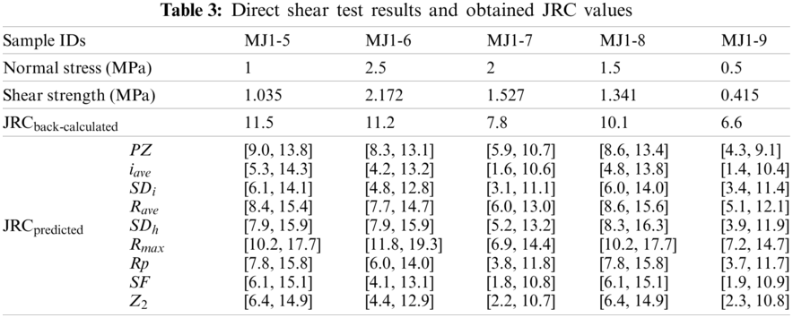
Figure 4: Three-dimensional surface models of sandstone joint samples (a) MJ1-5 (b) MJ1-6 (c) MJ1-7 (d) MJ1-8 (e) MJ1-9

The roughness parameter PZ of each extracted rock joint profile was first calculated along with the shear direction; then, the JRC value was calculated with the PZ-based NN function presented in Eq. (19). Then, the arithmetic mean of all 2D profiles extracted from the same sandstone sample was adopted to represent the 3D JRC values. This method has been confirmed to be effective by researchers [37–39]. The calculated JRC values of the collected sandstone joint samples based on the PZ-based NN function are presented in Tab. 3.

For comparison purposes, the commonly used statistical parameters, i.e., the Rave, Rmax, SDh, iave, SDi, Z2, Rp, and SF, were also calculated for the collected 112 rock joint profiles. The formulations for these statistical parameters can be seen in Tab. 1. Then the regression correlations between the JRC and selected statistical parameters are derived and shown in Fig. 5. Then, the NN functions based on the above-mentioned statistical parameters were also derived and listed as follows:

Figure 5: Correlations between the JRC and commonly used statistical parameters (a) iave (b) SDi (c) Rave (d) SDh (e) Rmax (f) Rp (g) SF (h) Z2

According to the derived statistical parameter-based NN functions, i.e., Eqs. (20)~(27), the JRC of the collected five joint samples were obtained. The calculated results are presented in Tab. 3 and plotted in Fig. 6. The results in Tab. 3 show that the PZ-based NN function and statistical parameters-based NN functions can approximate the JRC values for joint samples. However, the JRC values calculated by the commonly used statistical parameter-based NN functions are located in a much larger JRC range than the PZ-based NN function, which means the PZ-based NN function is much more sensitive and effective than the traditional approaches in determining the rock joint roughness. Especially, Fig. 6 shows that the statistical parameters may not present a correct JRC range for the sandstone joints. For example, the JRC ranges calculated by the Rmax based NN function for the sandstone joints MJ1-6, MJ1-8, and MJ1-9 deviate significantly from the experimental back-calculated JRC values. These differences in the JRC calculation results are that the PZ-based NN function comprehensively considers the effect of the shear direction, amplitude height, and inclination angle and effectively reflects the contribution of various scales of asperity components on the roughness. In contrast, the statistical parameters based NN functions only present one-sided characteristics of rock joint roughness (e.g., iave and Z2 only present the inclination angle of a joint profile), which contains more uncertainties in the JRC determination. Thus, the proposed approach, that is, the PZ-based NN function, can present much more effective JRC calculation results for natural rock joints.

Figure 6: Comparisons of JRC values calculated by different NN functions (a) MJ1-5 (b) MJ1-6 (c) MJ1-7 (d) MJ1-8 (e) MJ1-9

Figure 7: JRC values calculated for ten standard profiles based on mean trend correlations (a) JRC = 0.4 (b) JRC = 2.8 (c) JRC = 5.8 (d) JRC = 6.7 (e) JRC = 9.5 (f) JRC = 10.8 (g) JRC = 12.8 (h) JRC = 14.5 (i) JRC = 16.7 (j) JRC = 18.7

Generally, the JRC values have good correlations with commonly used statistical parameters. However, the indeterminate information of the JRC leads to variabilities in the predicted results of JRC regression correlations. Researchers usually adopt the mean trend of correlations to predict JRC values, while this subjected approach may result in biased results. Here, the mean trend correlations of the above-mentioned statistical parameters and the proposed PZ were used to present this information. As indicated in Fig. 7, all the predicted JRC values deviated from the true JRC values to some extent. Especially for the first standard profile with JRC = 0.4, negative JRC values were obtained by the mean trend correlations based on PZ, Z2, SF, and iave. This phenomenon once again shows that the traditional regression correlations cannot deal with the indeterminate information of the JRC.

Incomplete, imprecise, and indeterminate problems are generally encountered for the complex surface of rock joints. The NNs are preferred compared to fuzzy, rough, grey sets due to efficiency, flexibility, and easiness for expressing determinate and/or indeterminate information. Additionally, various scales of asperities are displayed on joint surfaces. The spectral analysis was adopted to simultaneously capture the contributions of the high and low-frequency asperity components in determining joint roughness. Through the combination of the NNs and spectral analysis, this paper proposed a new method to determine the JRC for rock joints accurately. The main conclusions are drawn as follows.

The JRC regression correlation based on commonly used statistical parameters could not handle the indeterminate information of the JRC. As a result, there were still significant deviations in calculated JRC values, although the JRC had a good correlation with the commonly used statistical parameters. Particularly, the absolute deviations for the calculated JRC results based on the Z2 and SF were larger than 70% for the profiles with true JRC values 0.4 and 2.8. These deviations can be attributed to the indeterminate information that exists in the joint roughness determination and the contribution differences of various scales of asperities on the joint roughness.

To overcome the limitations of the traditional JRC determination approaches, NN functions based on the spectral roughness parameter were derived based on 112 rock joint profiles collected from the literature. Then, the derived NN function was applied to determine the JRC values of 5 well-matched sandstone joint samples collected from the Majiagou rock landslide area. The comparison between the JRC results obtained from the proposed method and experimental results validated the effectiveness of the spectral analysis based NN functions. Additionally, comparisons made between the spectral analysis and common statistical parameters based on NN also demonstrated the advantage of spectral analysis. The combination of the NNs and spectral analysis can effectively address the indeterminate information that exists in the joint roughness and the contribution differences of various scales of asperities on the joint roughness.

In addition to the NN, the neutrosophic theory contains many other methods, such as neutrosophic sets, neutrosophic interval statistical numbers, and neutrosophic interval functions. They can also address the indeterminate information in the JRC determination process. In future work, we will further develop and investigate JRC determination approaches through other neutrosophic theories and compare the differences and efficiencies between different neutrosophic approaches.

Funding Statement: The authors would like to thank very much to the anonymous reviewers and editors whose constructive comments are helpful for this paper’s revision. This work is supported by Key Program of National Natural Science Foundation of China (No. 41931295) and General Program of National Natural Science Foundation of China (No. 41877258).

Conflicts of Interest: The authors declare that they have no conflicts of interest to report regarding the present study.

References

1. Yong, R., Li, C. D., Ye, J., Huang, M., Du, S. G. (2016). Modified limiting equilibrium method for stability analysis of stratified rock slopes. Mathematical Problems in Engineering, 2016(1), 1–9. DOI 10.1155/2016/8381021. [Google Scholar] [CrossRef]

2. Tang, H. M., Yong, R., Ez Eldin, M. A. M. (2016). Stability analysis of stratified rock slopes with spatially variable strength parameters: The case of Qianjiangping landslide. Bulletin of Engineering Geology and the Environment, 76(3), 839–853. DOI 10.1007/s10064-016-0876-4. [Google Scholar] [CrossRef]

3. Yong, R., Qin, J. B., Huang, M., Du, S. G., Liu, J. et al. (2018). An innovative sampling method for determining the scale effect of rock joints. Rock Mechanics and Rock Engineering, 52(3), 935–946. DOI 10.1007/s00603-018-1675-y. [Google Scholar] [CrossRef]

4. Yong, R., Ye, J., Li, B., Du, S. G. (2018). Determining the maximum sampling interval in rock joint roughness measurements using Fourier series. International Journal of Rock Mechanics and Mining Sciences, 101(1–2), 78–88. DOI 10.1016/j.ijrmms.2017.11.008. [Google Scholar] [CrossRef]

5. Wu, Q., Jiang, Y. F., Tang, H. M., Luo, H., Wang, X. et al. (2020). Experimental and numerical studies on the evolution of shear behaviour and damage of natural discontinuities at the interface between different rock types. Rock Mechanics and Rock Engineering, 53(8), 3721–3744. DOI 10.1007/s00603-020-02129-9. [Google Scholar] [CrossRef]

6. Muralha, J., Grasselli, G., Tatone, B., Blümel, M., Chryssanthakis, P. et al. (2014). ISRM suggested method for laboratory determination of the shear strength of rock joints: Revised version. Rock Mechanics and Rock Engineering, 47(1), 291–302. DOI 10.1007/s00603-013-0519-z. [Google Scholar] [CrossRef]

7. Barton, N. (1973). Review of a new shear-strength criterion for rock joints. Engineering Geology, 7(4), 287–332. DOI 10.1016/0013-7952(73)90013-6. [Google Scholar] [CrossRef]

8. Barton, N., Choubey, V. (1977). The shear strength of rock joints in theory and practice. Rock Mechanics, 10(1–2), 1–54. DOI 10.1007/BF01261801. [Google Scholar] [CrossRef]

9. Wang, L. Q., Wang, C. S., Khoshnevisan, S., Ge, Y. F., Sun, Z. H. (2017). Determination of two-dimensional joint roughness coefficient using support vector regression and factor analysis. Engineering Geology, 231(4), 238–251. DOI 10.1016/j.enggeo.2017.09.010. [Google Scholar] [CrossRef]

10. Liu, X., Zhu, W., Liu, Y., Yu, Q., Guan, K. (2021). Characterization of rock joint roughness from the classified and weighted uphill projection parameters. International Journal of Geomechanics, 21(5), 4021052. DOI 10.1061/(ASCE)GM.1943-5622.0001963. [Google Scholar] [CrossRef]

11. Yong, R., Fu, X., Huang, M., Liang, Q., Du, S. G. (2017). A rapid field measurement method for the determination of joint roughness coefficient of large rock joint surfaces. KSCE Journal of Civil Engineering, 22(1), 101–109. DOI 10.1007/s12205-017-0654-2. [Google Scholar] [CrossRef]

12. Xie, H., Wang, J. A. (1999). Direct fractal measurement of fracture surfaces. International Journal of Solids and Structures, 36(20), 3073–3084. DOI 10.1016/S0020-7683(98)00141-3. [Google Scholar] [CrossRef]

13. Kulatilake, P. H. S. W., Balasingam, P., Park, J., Morgan, R. (2006). Natural rock joint roughness quantification through fractal techniques. Geotechnical and Geological Engineering, 24(5), 1181–1202. DOI 10.1007/s10706-005-1219-6. [Google Scholar] [CrossRef]

14. Kulatilake, P. H. S. W., Du, S. G., Ankah, M. L. Y., Yong, R., Sunkpal, D. T. et al. (2021). Non-stationarity, heterogeneity, scale effects, and anisotropy investigations on natural rock joint roughness using the variogram method. Bulletin of Engineering Geology and the Environment, 80(8), 6121–6143. DOI 10.1007/s10064-021-02321-3. [Google Scholar] [CrossRef]

15. Li, Y., Xu, Q., Aydin, A. (2016). Uncertainties in estimating the roughness coefficient of rock fracture surfaces. Bulletin of Engineering Geology and the Environment, 76(3), 1153–1165. DOI 10.1007/s10064-016-0994-z. [Google Scholar] [CrossRef]

16. Ye, J., Yong, R., Liang, Q. F., Huang, M., Du, S. G. (2016). Neutrosophic functions of the joint roughness coefficient and the shear strength: A case study from the pyroclastic rock mass in Shaoxing City. China Mathematical Problems in Engineering, 2016(1), 1–9. DOI 10.1155/2016/4825709. [Google Scholar] [CrossRef]

17. Du, S. G. (1998). Research on complexity of surface undulating shapes of rock joints. Journal of China University of Geosciences, 9(1), 86–89. [Google Scholar]

18. Wang, C. S., Wang, L. Q., Karakus, M. (2019). A new spectral analysis method for determining the joint roughness coefficient of rock joints. International Journal of Rock Mechanics and Mining Sciences, 113, 72–82. DOI 10.1016/j.ijrmms.2018.11.009. [Google Scholar] [CrossRef]

19. Ficker, T., Martišek, D. (2016). Alternative method for assessing the roughness coefficients of rock joints. Journal of Computing in Civil Engineering, 30(4), 4015059. DOI 10.1061/(ASCE)CP.1943-5487.0000540. [Google Scholar] [CrossRef]

20. Smarandache, F. (2013). Introduction to neutrosophic measure, neutrosophic integral, and neutrosophic probability. Craiova: Sitech Publishing House. [Google Scholar]

21. Smarandache, F. (1998). Neutrosophy: Neutrosophic probability, set, and logic. Rehoboth: American Research Press. [Google Scholar]

22. Smarandache, F. (2014). Introduction to neutrosophic statistics. Craiova: Sitech & Education Publishing. [Google Scholar]

23. Ye, J., Cui, W. (2019). Neutrosophic compound orthogonal neural network and its applications in neutrosophic function approximation. Symmetry, 11(2), 147. DOI 10.3390/sym11020147. [Google Scholar] [CrossRef]

24. Du, S. G., Yong, R., Ye, J. (2020). Subtraction operational aggregation operators of simplified neutrosophic numbers and their multi-attribute decision making approach. Neutrosophic Sets and Systems, 33, 157–168. DOI 10.5281/zenodo.3782881. [Google Scholar] [CrossRef]

25. Ye, J., Song, J. M., Du, S. G. (2020). Correlation coefficients of consistency neutrosophic sets regarding neutrosophic multi-valued sets and their multi-attribute decision-making method. International Journal of Fuzzy Systems, 1–8. DOI 10.1007/s40815-020-00983-x. [Google Scholar] [CrossRef]

26. Chen, J., Ye, J., Du, S. G., Yong, R. (2017). Expressions of rock joint roughness coefficient using neutrosophic interval statistical numbers. Symmetry, 9(7), 123. DOI 10.3390/sym9070123. [Google Scholar] [CrossRef]

27. Ye, J., Chen, J., Yong, R., Du, S. G. (2017). Expression and analysis of joint roughness coefficient using neutrosophic number functions. Information–An International Interdisciplinary Journal, 8(2), 69. DOI 10.3390/info8020069. [Google Scholar] [CrossRef]

28. Karamaşa, Ç., Demir, E., Memiş, S., Korucuk, S. (2021). Weighting the factors affectıng logıstıcs outsourcıng. Decision Making: Applications in Management and Engineering, 4(1), 19–33. DOI 10.31181/dmame2104019k. [Google Scholar] [CrossRef]

29. Aslam, M., Bantan, R. A. R., Khan, N. (2021). Design of tests for mean and variance under complexity–An application to rock measurement data. Measurement, 177, 109312. DOI 10.1016/j.measurement.2021.109312. [Google Scholar] [CrossRef]

30. Aslam, M. (2019). A new method to analyze rock joint roughness coefficient based on neutrosophic statistics. Measurement, 146, 65–71. DOI 10.1016/j.measurement.2019.06.024. [Google Scholar] [CrossRef]

31. Du, S. G., Ye, J., Yong, R., Zhang, F. (2020). Simplified neutrosophic indeterminate decision making method with decision makers’ indeterminate ranges. Journal of Civil Engineering and Management, 26(6), 590–598. DOI 10.3846/jcem.2020.12919. [Google Scholar] [CrossRef]

32. Allen, R. L., Mills, D. (2004). Signal analysis: Time, frequency, scale, and structure. USA: John Wiley & Sons. [Google Scholar]

33. Li, Y., Zhang, Y. (2015). Quantitative estimation of joint roughness coefficient using statistical parameters. International Journal of Rock Mechanics and Mining Sciences, 77, 27–35. DOI 10.1016/j.ijrmms.2015.03.016. [Google Scholar] [CrossRef]

34. Yong, R., Ye, J., Liang, Q. F., Huang, M., Du, S. G. (2017). Estimation of the joint roughness coefficient (JRC) of rock joints by vector similarity measures. Bulletin of Engineering Geology and the Environment, 77(2), 735–749. DOI 10.1007/s10064-016-0947-6. [Google Scholar] [CrossRef]

35. Grasselli, G., Wirth, J., Egger, P. (2002). Quantitative three-dimensional description of a rough surface and parameter evolution with shearing. International Journal of Rock Mechanics and Mining Sciences, 39(6), 789–800. DOI 10.1016/S1365-1609(02)00070-9. [Google Scholar] [CrossRef]

36. Marache, A., Riss, J., Gentier, S., Chilès, J. P. (2002). Characterization and reconstruction of a rock fracture surface by geostatistics. International Journal for Numerical and Analytical Methods in Geomechanics, 26(9), 873–896. DOI 10.1002/nag.228. [Google Scholar] [CrossRef]

37. Tatone, B. S. A., Grasselli, G. (2010). A new 2D discontinuity roughness parameter and its correlation with JRC. International Journal of Rock Mechanics and Mining Sciences, 47(8), 1391–1400. DOI 10.1016/j.ijrmms.2010.06.006. [Google Scholar] [CrossRef]

38. Zhang, G. C., Karakus, M., Tang, H. M., Ge, Y. F., Zhang, L. (2014). A new method estimating the 2D joint roughness coefficient for discontinuity surfaces in rock masses. International Journal of Rock Mechanics and Mining Sciences, 72(B8), 191–198. DOI 10.1016/j.ijrmms.2014.09.009. [Google Scholar] [CrossRef]

39. Ge, Y. F., Lin, Z., Tang, H. M., Zhao, B. (2021). Estimation of the appropriate sampling interval for rock joints roughness using laser scanning. Bulletin of Engineering Geology and the Environment, 80(5), 3569–3588. DOI 10.1007/s10064-021-02162-0. [Google Scholar] [CrossRef]