Computer Modeling in Engineering & Sciences

DOI: 10.32604/cmes.2021.017268

ARTICLE

Modelling of Contact Damage in Brittle Materials Based on Peridynamics

Jingjing Zhao1,*, Guangda Lu2, Qing Zhang3 and Wenchao Du4

1Nanjing Institute of Railway Technology, Nanjing, 210031, China
2Tongji University, Shanghai, 200092, China
3Department of Engineering Mechanics, Hohai University, Nanjing, 211100, China
4Nanjing High Speed Gear Manufacturing Co., Ltd., Nanjing, 211100, China
*Corresponding Author: Jingjing Zhao. Email: zhaojingjing198678@126.com
Received: 27 April 2021; Accepted: 11 August 2021

1  Introduction

Glass is a highly homogeneous brittle material and it can be made into any shape and mass produced due to its homogeneity. Hence, glass materials are widely used in construction, transportation, shipping, aviation, aerospace and other industries. However, the glass is extremely easy to break when its surface is subjected to impact load. Effectively revealing the mesoscopic failure mechanism of glass under low-velocity impact loads is of great importance to improve its resistance and safety.

In the early days, many scholars investigated the damage of glass under impact, mainly focusing on the crack initiation, propagation, and crack development patterns of glass through a series of experimental studies [1–6]. In 1931, Andrews [1] pointed out that a force threshold is found for the crack formation of glass under impact load. Roesler [2] considered the conical indentation of a glass specimen and measured its fracture energy to verify Griffith [3] energy balance condition for brittle material cracking. Knight et al. [4], Chaudhri et al. [5] studied the crack development patterns of glass under medium and high-speed loading by changing the impact velocity of iron ball. The results show that the crack appears in the non-loading section, and the Hertzian cone angle of the crack zone varies with the loading speed. Ball et al. [6] observed that glass specimens exhibit a star-shaped fragmentation failure mode under low-speed conditions. In recent years, Bouzid et al. [7], Nyongue et al. [8], and Daryadel et al. [9] conducted relevant quantitative experimental analysis on the dynamic response and fracture criterion for glass under impact loading. The failure mechanism for different types of glass is realized in the work of Kumar et al. [10]. These test results reveal the response law and failure mechanism of glass as a typical brittle material under impact load from different aspects.

With the development of computers, numerical simulation methods have been widely used to reproduce and explain the phenomena observed in experiments. Numerical models based on traditional continuum mechanics, such as finite element method [11] and boundary element method [12], are gradually used in many experimental studies. However, for discontinuities, such as crack bifurcation in solid materials and structures, traditional numerical methods are faced with the problems of singularity and low computational efficiency. The use of grid reconstruction [13] or the method of adding a cohesive element [14] in the finite element would cause to grid-dependent results. The partition algorithm [15] and fictitious crack model [16] adopted by the boundary element method (BEM) have similar limitations to the finite element method in the analysis of crack propagation problems. Therefore, researchers have proposed the extended finite element method [17]. Compared with the traditional finite element method, it reduces the strict requirements on the mesh discontinuity. However, in the construction of enrichment function, the extended finite element method needs to know the characteristics of the problem to be solved in advance. This condition is relatively demanding for complex problems, such as crack branching and multi-crack intersection. In recent years, many researchers have studied the contact damage of brittle materials under impact load. Oliveira et al. [18] proposed an alternative BEM formulation to model the cohesive stresses through the domain term of the direct integral. Wang et al. [19] proposed a field-enriched finite element method to simulate the failure process of rocks. Kouet et al. [20] presented a bonded-particle methodology to investigate the crack growth and crack branching. Bo et al. [21,22] developed some explicit Galerkin formulations which can capture ductile fractures during high-speed impacts and simulate fracture of a plate under impact loads.

To solve contradiction between the continuity assumption and the discontinuity phenomenon of the failure problem, Silling [23] proposed a nonlocal method called peridynamics (PD) [24] to described the motion process of the material points through an integral equation. In the development of the peridynamics, researchers have conducted numerous quantitative analyses on the brittle fracture of polycrystalline materials [25], impact failure of shale materials [26], and the thermal brittleness and failure of glass plate under impact [27–29], and the problem of interaction between ice and seawater [30]. Those results show that peridynamics does not have the singularity problem when analyzing the failure problem and can simulate the whole process of the material, including macroscopic crack initiation, propagation, and final failure. The above simulation of failure is based on the bond-based peridynamics theory (BBPD). However, bond-based peridynamics theory has some problems, such as the limitation of Poisson’s ratio and the lack of connection with traditional continuum theory. Silling et al. [31–32] proposed an ordinary state-based peridynamic theory (OSBPD) and a non-ordinary state-based peridynamics(NOSB PD). Both of them inherit the advantages of BBPD for solving discontinuous problems, and have a similar definition of state quantities to traditional physical quantities. To address the limitations of material calculation scale. Breitenfeld et al. [33], O’Grady et al. [34], and Chowdhury et al. [35] supplemented and developed the OSBPD theory. Song et al. [36] proposed a state-based peridynamic model by using adaptive particle refinement to simulate the formation of water ice crater under impact loads. Zhou et al. [37] developed a 2D elastoplastic model of the ordinary state-based peridynamic theory to analyze the plastic zone of the crack tip of rock material. Wu et al. [38] proposed a concrete impact failure model based on NOSBPD theory. In recent years, many scholars began to study the contact model based on PD method. Xin et al. [39] developed a NOSBPD model for brittle fracture to simulate the edge-on impact and drop ball test and discussed the contact algorithm between the projectile and target. Littlewood et al. [40] summarized the simulation results of finite element method and peridynamics. A combined approach of finite element method and peridynamics is utilized via a contact algorithm. Ye et al. [41] proposed a continuous contact detection algorithm to simulate the brittle failure behavior of ice during the contact between propeller and ice. This algorithm can well capture the ice damage characteristics. Kamensky et al. [42] summarized several existing peridynamic contact friction models and introduced a state-based nonlocal friction formulation to demonstrate the properties of various peridynamic contact models through some impact and penetration problems. Silling et al. [43] proposed a new PD model to simulate the elastoplastic response, creep, and fracture. In the case of small deformation, this model is consistent with classical Hertz contact analysis. Wang et al. [44] proposed a 3D conjugated bond-pair-based peridynamic model to simulate the failure characteristics of rock materials with different forms of central fissure.

This paper presents a new contact damage model based on the OSBPD theory for glass by introducing a contact force function. The arrangement of the rest sections is as follows. In Section 2, the governing equations based on OSBPD theory are described in brief, followed by the contact model and algorithm. In Section 3, the Hertz contact (nonembedded contact) problem is simulated, and the elastic contact force is determined by adjusting the penalty factor. The proposed model verifies the feasibility of penalty-based method to simulate the contact problem of glass. In Section 4, the failure process of glass specimen under impact is simulated, and two loading methods, drop ball test (DBT) and split Hopkinson pressure bar (SHPB), are considered. The numerical results agree well with the experimental results, which verifies the effectiveness of the proposed model.

2  Methodology

2.1 Fundamentals of Peridynamics Theory

In PD theory, an object occupies a region υ (namely the reference configuration shown in Fig. 1). A certain interaction (nonlocal interaction) is assumed between a particle x and other particle x′ within a horizon Hx={x′:‖x′−x‖≤δ}⊂υ, where δ is the truncation radius. Let H0=Hx for convenience because Hx has nothing to do with time. Supposed a region D⊂Hx is occupied by a particle x on the object. By defining the relative position state vector X_⟨x′−x⟩=x′−x and relative displacement state vector U_⟨x′−x⟩=u′−u, where u is the displacement of the particle x, the deformation state vector is expressed as

Y_⟨x′−x⟩=X_⟨x′−x⟩+U_⟨x′−x⟩=y′−y (1)

where y is the position of particle x after deformation. The force state vector between x and x′ can be defined as

T_[x]⟨X_⟩=t_[x]M_⟨X_⟩=t[x]Y_⟨X_⟩‖Y_⟨X_⟩‖ (2)

where M_⟨X_⟩ is the state vector of the deformation direction, showing the direction of the interaction force between the material points is consistent with its relative deformation direction; t_[x] is the force state scalar. The force of particle x exerted by its neighboring particle x′ is expressed as

t(X_,U_,t)=T_[x,t]⟨X_⟩−T_[x′,t]⟨−X_⟩ (3)

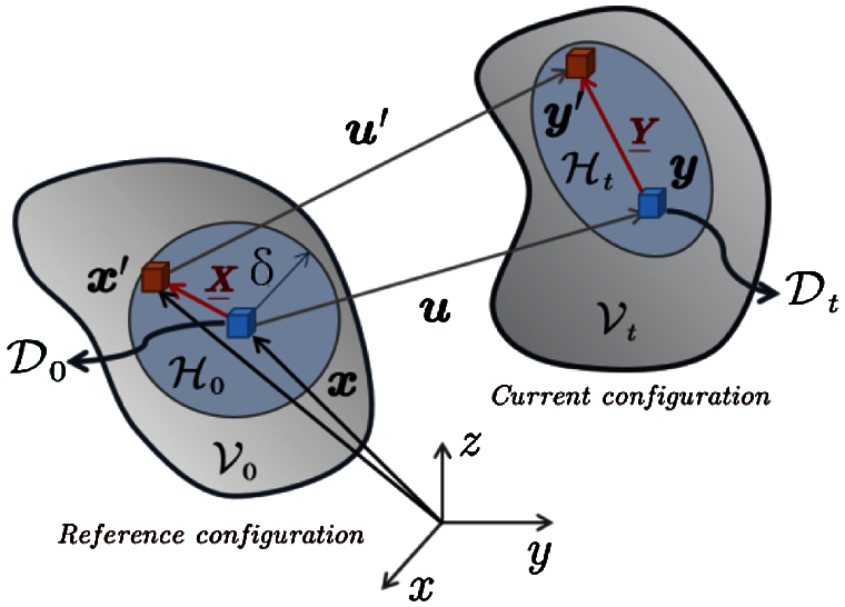
Figure 1: Reference configuration of particle movement

Therefore, a momentum balance equation at particle x is defined as

ρtu¨(x,t)=∫H0{T_[x,t]⟨X_⟩−T_[x′,t]⟨−X_⟩}dV′+b(x,t) (4)

The above formula is the governing equation of peridynamics [31–32], and its above derivation shows that the peridynamics theory still belongs to the Lagrangian system. The difference from the traditional continuum mechanics is that it considers the nonlocal interaction between the particles.

∫H0tdV′←∫∂DttdV=∫Dt∇⋅σdV (5)

where σ is the stress tensor.

2.2 Force State of State-Based Peridynamics Theory

Let x_⟨X_⟩=‖X_‖ denote the initial length state scalar between the interacting particles, The weighted volume m is defined as

m[x]=∫H0ω⟨‖X_‖⟩x_⟨X_⟩x_⟨X_⟩dV′ (6)

where ω_⟨‖X_‖⟩ is the influence state and describes the relative degree of interactions between particles. The elongation [31] between a pair of material points is defined as

e_⟨X_⟩=‖Y_⟨X_⟩‖−‖X_‖ (7)

The volume dilatation θ is defined as

θ(e)=3m[x]∫H0ω⟨‖X_‖⟩x_⟨X_⟩e_⟨X_⟩dV′ (8)

In accordance with elastic mechanics, the extension scalar state e_⟨X_⟩ can be decomposed into isotropic part

e_i⟨X_⟩=θx_⟨X_⟩3 (9)

and deviatoric part

e_d⟨X_⟩=e_⟨X_⟩−e_i⟨X_⟩ (10)

Therefore, the elastic energy density contains two parts

W(e_i,e_d)=12Kθ2+12α∫H0ω_⟨X_⟩e_d⟨X_⟩e_d⟨X_⟩dVx′ (11)

Correspondingly, the scalar force t_ can be expressed as

t_=t_i+t_d=∂W∂e_i+∂W∂e_d=∂W∂θ∂θ∂e_i+∂W∂e_d (12)

In accordance with the energy equivalence between the deformation energy density (11) and the strain energy density of classical elasticity, t_ can be obtained as [31]

t_[x,t]=3Kθm[x]ω_⟨‖X_‖⟩x_⟨X_⟩+15Gm[x]ω_⟨‖X_‖⟩e_d⟨X_⟩ (13)

The above formula is the force state of state-based peridynamics theory, which includes traditional material parameters, such as bulk modulus K and shear modulus G. For the damaged material points, the scalar function [23] is defined as

D(x,t)=1−∫H0μ(X_,Y_,t)x_⟨X_⟩x_⟨X_⟩dV′∫H0x_⟨X_⟩x_⟨X_⟩dV′ (14)

where μ is a scalar function, and it is defined as

μ(X_,Y_,t)={10ifs(X_,Y_,t)≤s0else (15)

where s is the fracture judgment parameter and s0 is the corresponding critical value. If the extension scalar state is selected as the basis for judging whether the bond between two material points is broken, then s and s0 are defined as

s=‖Y_⟨X_⟩‖−‖X_‖‖X_‖,s0=5G09Kδ (16)

where G0 [45] is the energy release rate. For the local damage defined by Eq. (14), the damage between material point pairs is shown in Fig. 2.

Figure 2: Damage between material point pairs when D≈0.5

2.3 Contact Model of Peridynamics

The contact problem of two objects shown in Fig. 3 is considered. Let xA be the coordinate of any material point P on the ScA. The distance between this point P and the nearest point Q(xB) on ScB can be expressed as

gtn=min‖xA−xB‖=(xA−xB)⋅etn (17)

where the unit normal etn of the contact surface is

etn=e1×e2‖e1×e2‖ (18)

Considering the impenetrability of contact, any material point on ScA should satisfy gtn≥0, where gtn>0 indicates that point P is separated from surface ScB, gtn=0 denotes contact, and gtn<0 represents that υtA and υtB penetrate each other. This condition is not allowed. Therefore, if the impenetrability is satisfied at time t, then the following condition should be met at time t+Δt

gt+Δtn=(xt+ΔtA−xt+ΔtB)⋅et+Δtn≥0 (19)

Note xt+ΔtA=xtA+uA and xt+ΔtB=xtB+uB, so

gt+Δtn=unA−unB+gtn≥0 (20)

where

{unA=uA⋅et+ΔtnunB=uB⋅et+Δtngtn=(xtA−xtB)⋅et+Δtn (21)

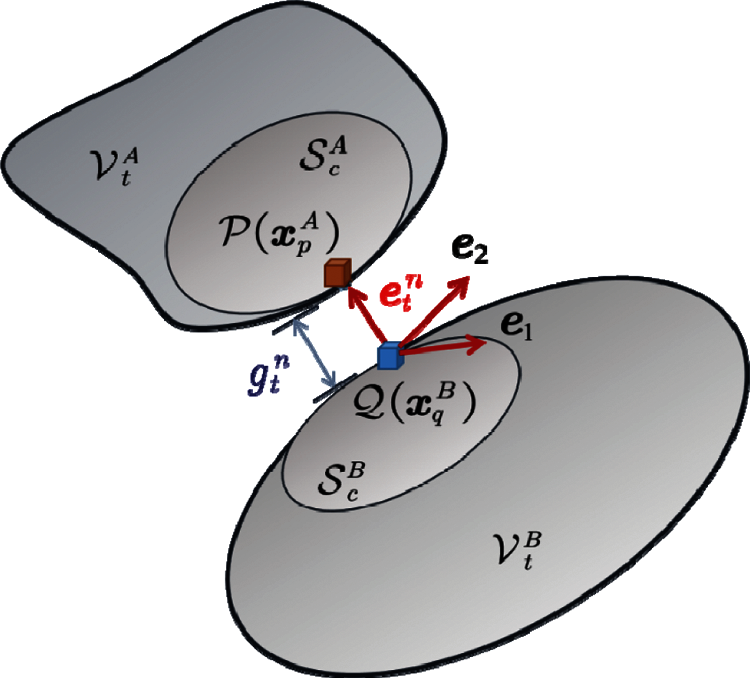
Figure 3: Contact point pair and the distance between them

The energy function, which includes A and B systems, is expressed as

Π=Π0+Πcf+Πcp (22)

where Π0 is the energy function without considering the contact force and contact conditions. For A and B, δΠ0=0, which is equivalent to the Eq. (7), where Πcf is the potential energy function of contact force. These contact forces are the acting force and reaction force. Thus, we have

Πcf=∑kA,B∫Sckfcnk⋅unkdS=∫ScABfcnA(unA−unB)dS (23)

where ScAB=ScA∪ScB. Πcp is the additional functional of the introduced contact condition Eq. (19) and is defined as

Πcp=∫ScABcn(unA−unB+gtn)2dS (24)

where cn is the penalty factor. Let δΠ=0, we have

fcnA=−fcnB=−cn(unA−unB+gtn)=−cngtn+Δt (25)

For a certain contact deformation body, if its contact surface is Sc, then the contact force is

Fc=∫Scfc(x,t)dS,x∈Sc (26)

where fc=(fc1 fc2 fcn)T and fc1=fc2=0. Once the object is in contact, the contact force is applied to the material point on the contact surface in the form of body force density, that is

fc(x,t)=∫Dtb(x,t)dV (27)

The contact force is related to the selection of the penalty factor. In theory, the larger the penalty factor cn, the higher the calculation accuracy, and the closer to the nonpenetration condition. This condition will be discussed in detail in the numerical solution process and specific examples. The penalty factor is collectively referred to as the contact force modulus in this paper.

2.4 Numerical Discretization and Solution

Regarding the spatial discretization, peridynamics divides the material uniformly into a cubic lattice of side length Δx, and the volume for any material point is ΔV (Fig. 4). Therefore, all material points in H0 can be defined as

Fi=(Γ‖xj−xi‖≤δ) (28)

Correspondingly, the discretization of the motion equation considering the contact force in the space domain is

ρΔVu¨i=∑Γ∈Fit(xj−xi,uj−ui)ΔV2+fc(xi,t)=∑Γ∈Fi{T_[xi,t]⟨xj−xi⟩−T_[xj,t]⟨xi−xj⟩}ΔV2+fc(xi,t) (29)

Similar discrete operations are applied to the weighted volume m[x] and volume dilatation θ.

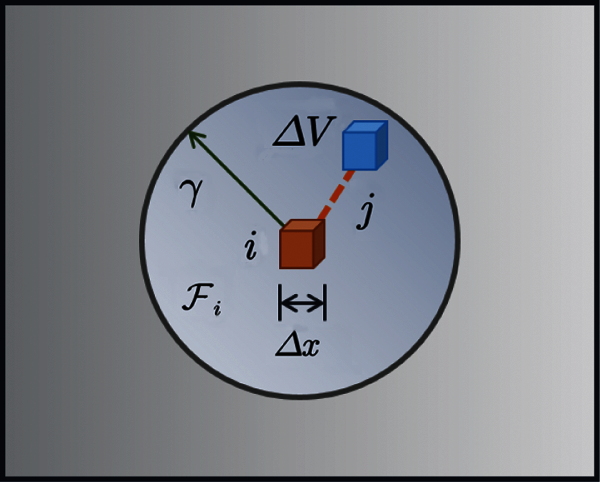
Figure 4: Discretization of spatial domain

Let uin=u(xi,tn) and time step Δt=tn−tn−1. The the formula of central difference scheme is obtained as

u¨in=uin+1−2uin+uin−1Δt2 (30)

Substituting the above formula into the Eq. (29). Thus, we have

uin+1=Δt2ρΔV[∑Γ∈Fit(xj−xi,ujn−uin)ΔV2+fcin]+2uin−uin−1 (31)

where fcin=fc(xi,tn). The difference scheme Eq. (31) should satisfy the Courant–Friedrichs–Lewy (CFL) stability condition. Let

C(X_)=∂t(X_,U_,t)∂U_ (32)

The time step should satisfy [33]

Δt<2ρ∑Γ∈FiCijΔVj (33)

The virtual rigid “spring” is added, that is, the rigidity of contact area Sc is improved. Eq. (33) is modified as

Δt<2ρ∑Γ∈FiCijΔVj+cn (34)

The value of penalty factors cn is discussed in the following calculation examples.

3  Verification of the Elastic Contact Problem

The Hertzian contact (no embedded contact) is considered, as shown in Fig. 5. The size parameters of the deformation body are L=B=1.6 m and H=0.8 m. The elastic modulus and Poisson’s ratio of the material are E=10 GPa and ν=0.25. The mass density is ρ=2400 kg/m3. The radius of the rigid sphere is set as R=0.2 m, and 2R/L≤3 approximately satisfies the assumption of semi-infinite deformation body. The fixed horizon size is set as δ=3Δx. The time step is set as Δt=1×10−7s. For the theoretical solution of this problem, the derivation can be found in the Appendix.

Figure 5: Hertzian contact problem

When the rigid sphere is in contact with the deformable body at a constant speed v=10 m/s (it can be regarded as a quasi-static problem), cn=5×106,1×107,5×107,1×108,5×108,1×109 are used for calculation to analyze the influence of contact modulus cn on the result. The discrete distance of the deformable body is set as Δx=0.01 m. The results of embedded distance de and contact force Fc corresponding to indentation depth d are shown in Figs. 6 and 7. As shown in Figs. 6 and 7, the contact force gradually approaches the theoretical solution with the increase in contact modulus cn. Therefore, for non-embedded contact problems, the value of contact modulus cn should be as large as possible to satisfy the computer truncation error and the stability requirements of differential solution.

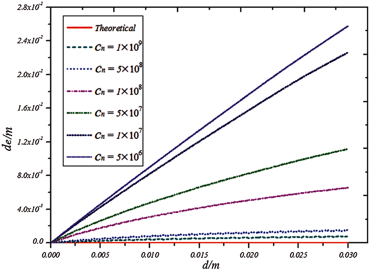
Figure 6: Graph of embedded distance de corresponding to indentation depth d

For the case of cn=1×109, the displacement nephogram of deformation body in y direction at time t=1×10−3,2×10−3,3×10−3s is drawn in Fig. 8. For the contact problem of a rigid sphere, the contact surface is arc-shaped, and its displacement decreases outward along the center of the contact surface, which is also consistent with the actual situation.

The discrete distance is still set as Δx=0.01 m, and the contact modulus is taken as cn=1×109. The radius of rigid sphere is changed by increment ΔR=0.05 m. When the indentation depth of the rigid sphere is d=0.02 m, contact force Fc is plotted in Fig. 9. With the increase in radius of the rigid sphere, contact force Fc is closer to the corresponding theoretical solution. When R=0.15 m and the relative discrete size is set as Δχ=Δx/2R=1/30, the calculation error of contact force Fc is 6.9915. When R=0.2 m and Δχ=1/40, the calculation error of contact force Fc drops to 0.1377. The calculation error of the contact force decreases with the decrease in the relative discrete size. The smaller the relative discrete size (the more discrete material points), the more time consuming the calculation. As shown in Fig. 9, the effect of improving the error is unremarkable when the relative discrete size is less than a certain critical value. When R=0.2 m and the contact modulus of the rigid sphere is still taken as cn=1×109, change the discrete distance of the material points and take Δx=0.1,0.08,0.05,0.04,0.02,0.01 m. The calculation results are shown in Fig. 10. A similar conclusion can be obtained, that is, the calculation error of the contact force gradually decreases with the decrease in distance between the material points.

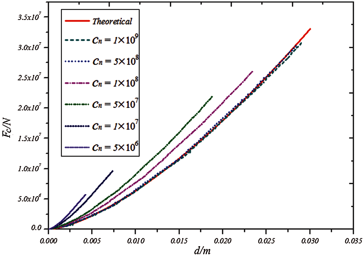
Figure 7: Relationship between contact force Fc and indentation depth d

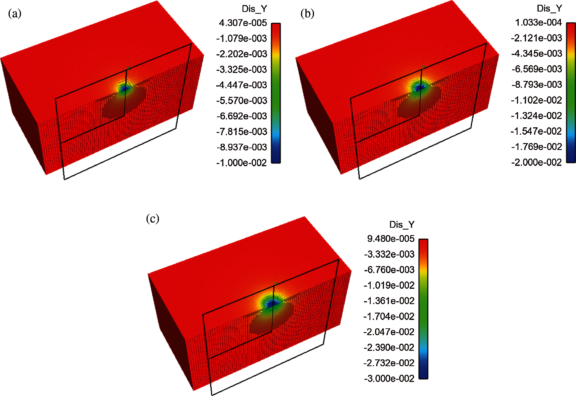
Figure 8: Displacement profile of the deformable body (a) t=1×10−3 s (b) t=2×10−3 s (c) t=3×10−3 s

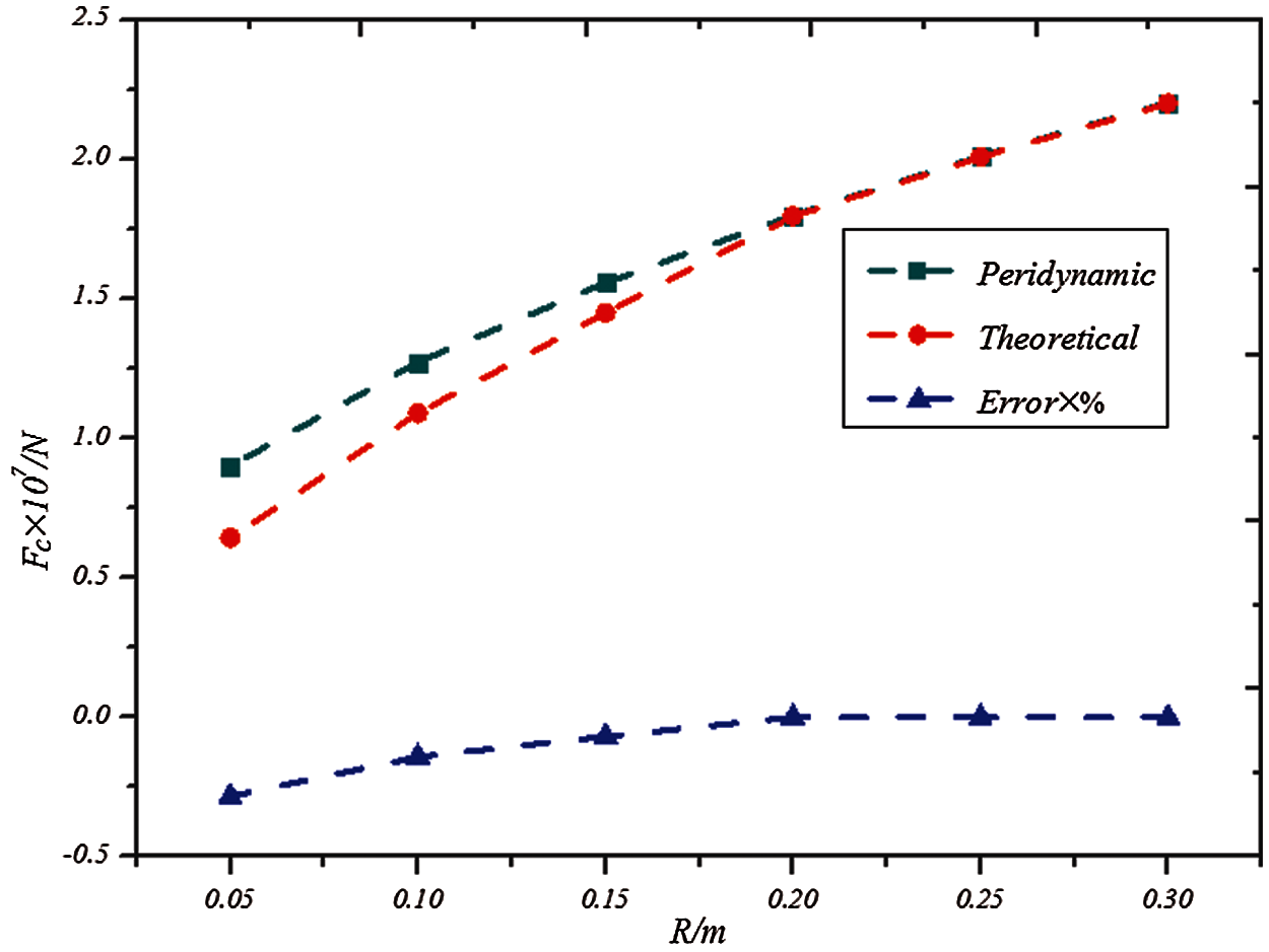
Figure 9: Plots of the contact force vs. the radius of rigid sphere

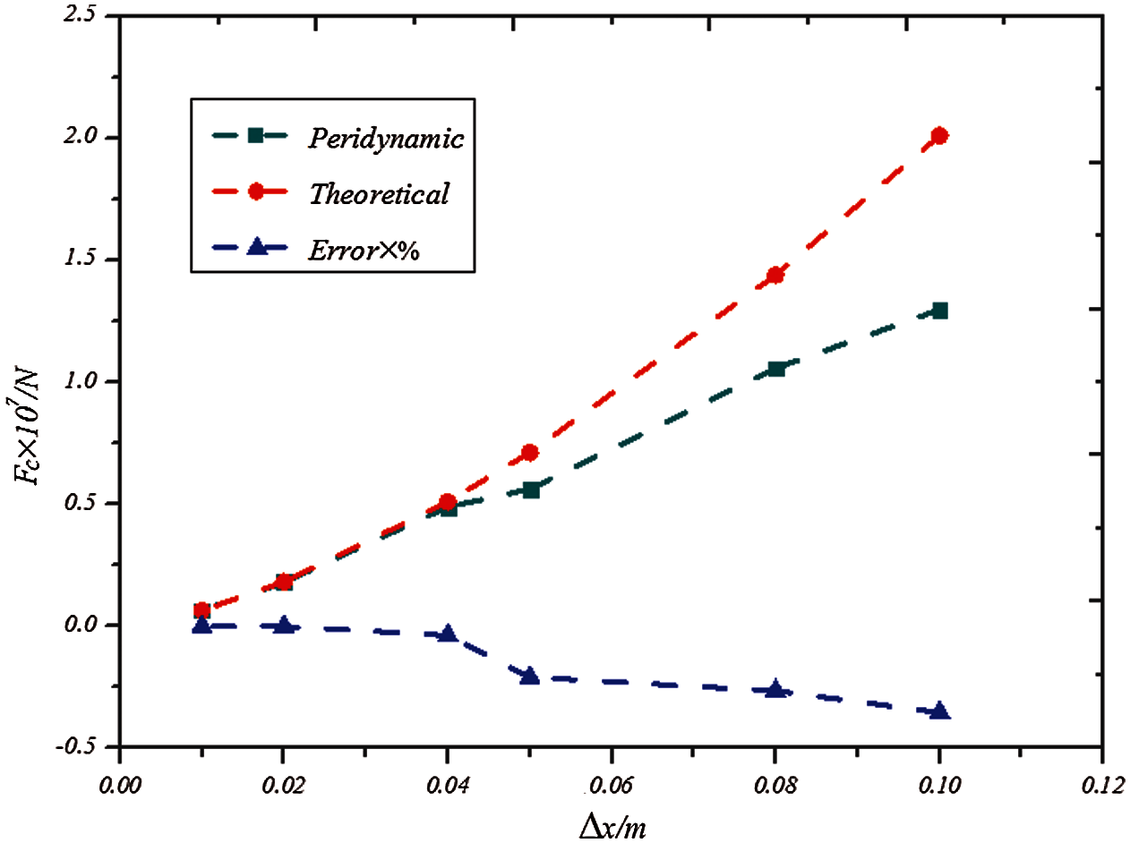
Figure 10: Plots of the contact force vs. the discrete distance

In summary, the influencing factors in the contact model of peridynamics are discussed and compared with the theoretical solution. The penalty-based method can be used to simulate the contact problem well by selecting the appropriate relative discrete size and the contact modulus. This process meets the requirements of computer truncation error and stable calculation. Therefore, on the basis of experience and the calculation results of this case, the calculation formula of contact modulus can be given as follows:

cn=αEΔx (35)

The range of adjustment coefficient α is from 1 to 50; E is the elastic modulus; Δx is the discrete distance of material points.

4  Contact Failure of Glass Specimen under Impact

Float glass material [7] is selected for analysis. The elastic modulus is E=70 GPa, the Poisson’s ratio is ν=0.23, the mass density is ρ=2508 kg/m3, and the critical energy release rate is set as G0=8 J/m2. The length and width of the glass sample are the same as L=B=100 mm, and the thickness is H=5 mm. For the simulations of DBT and SHPB, the models are shown in Figs. 11 and 12. In the simulation of DBT, the mass of the iron ball is 55 gr.(3.564 g), and the mass density is ρ=7860 kg/m3. The pressure bar is made of aluminum in the simulation of SHPB. Its elastic modulus is E=71 GPa, the Poisson’s ratio is ν=0.33, and the mass density is ρ=2900 kg/m3.

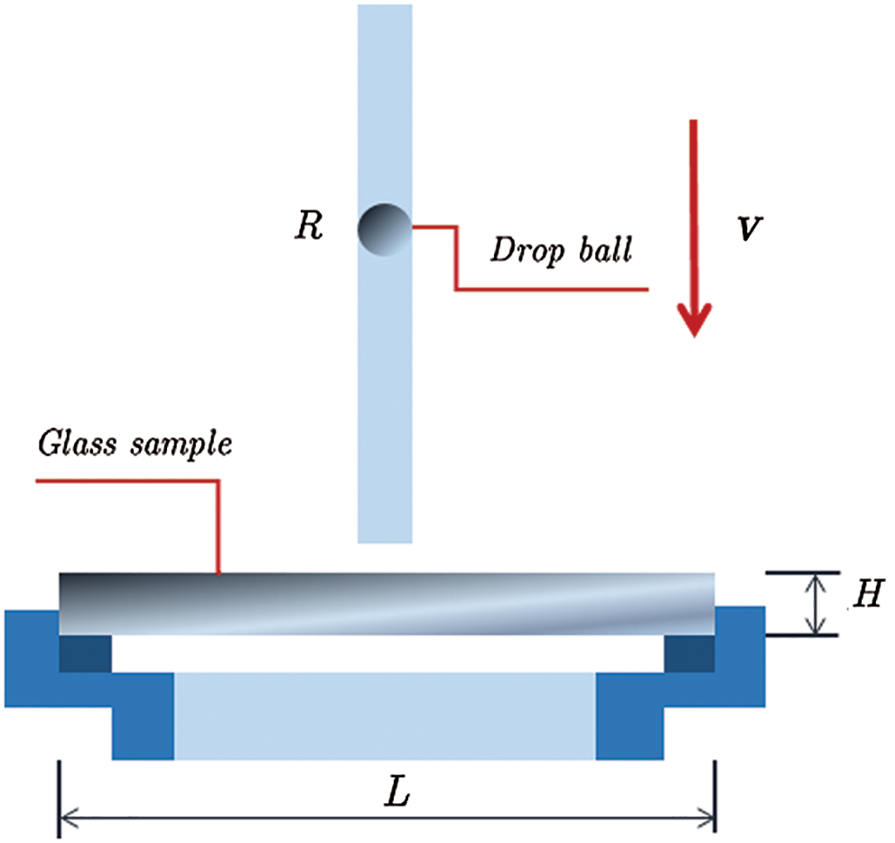
Figure 11: Geometric model of DBT [7]

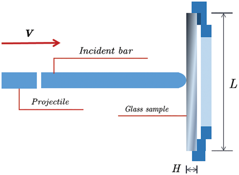
Figure 12: Geometric model of SHPB [7]

In the analysis of peridynamics, the contact modulus is taken as cn=1×109, and the discrete distance of glass samples is Δx=0.5 mm when the penalty-based method is used to calculate the above two models. The time step value is Δt=1×10−8 s. The low loading rate of DBT and the high loading rate of SHPB are considered. The results are shown in Figs. 13 and 14. For low loading rate (v=1 m/s) in Fig. 13, the final damage form is mainly a small amount of fragments. For the high-speed impact of SHPB, the sample appears to be broken. The simulation results are in good agreement with the test results (Fig. 15).

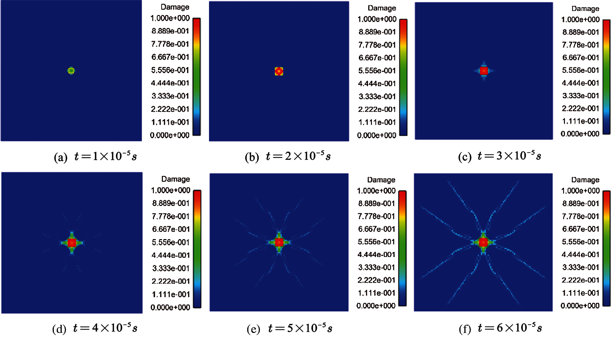
Figure 13: Damage of DBT model at different times (v=1 m/s) (a) t=1×10−5 s (b) t=2×10−5 s (c) t=3×10−5 s (d) t=4×10−5 s (e) t=5×10−5 s (f) t=6×10−5 s

Considering the low loading rate (v=3 m/s) of DBT and the high loading rate (v=30 m/s) of SHPB, the comparison between the two simulations and test results are shown in Fig. 16. The proposed contact damage model can deal with the impact failure of glass qualitatively and quantitatively. The curve of contact force vs. indentation depth is shown in Fig. 17. The comparison of DBT and SHPB results by using different load rates shows that the impact speed increases with the increase in impact speed.

The damage of glass specimens in different times is shown in Fig. 18. With the increase in loading speed, the damage time becomes shorter, and the damage degree becomes more serious. The simulation results are consistent with the experimental results. Therefore, the contact model of peridynamics can well simulate the failure of brittle materials under impact conditions.

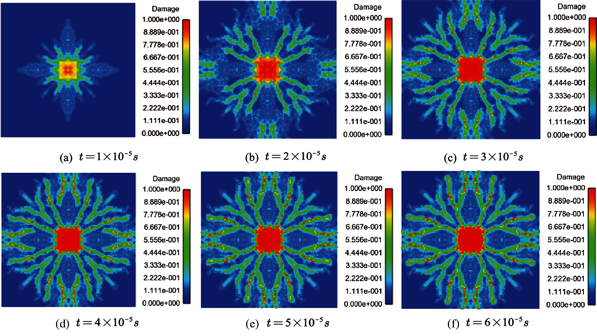
Figure 14: Damage of SHPB model at different times (v=20 m/s) (a) t=1×10−5 s (b) t=2×10−5 s (c) t=3×10−5 s (d) t=4×10−5 s (e) t=5×10−5 s (f) t=6×10−5 s

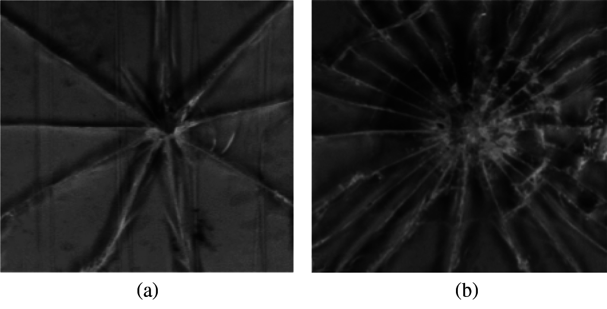
Figure 15: Experimental results [7] (a) Low loading rate of DBT (b) High loading rate of SHPB

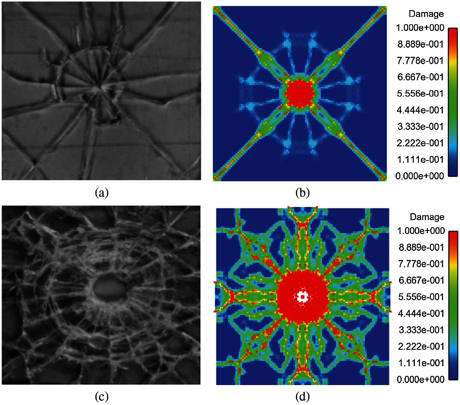
Figure 16: Comparison of experimental results and simulation results (a) Experimental results of DBT [7] (b) Peridynamics results of DBT (v=3 m/s) (c) Experimental results of SHPB [7] (d) Peridynamics results of SHPB (v=30 m/s)

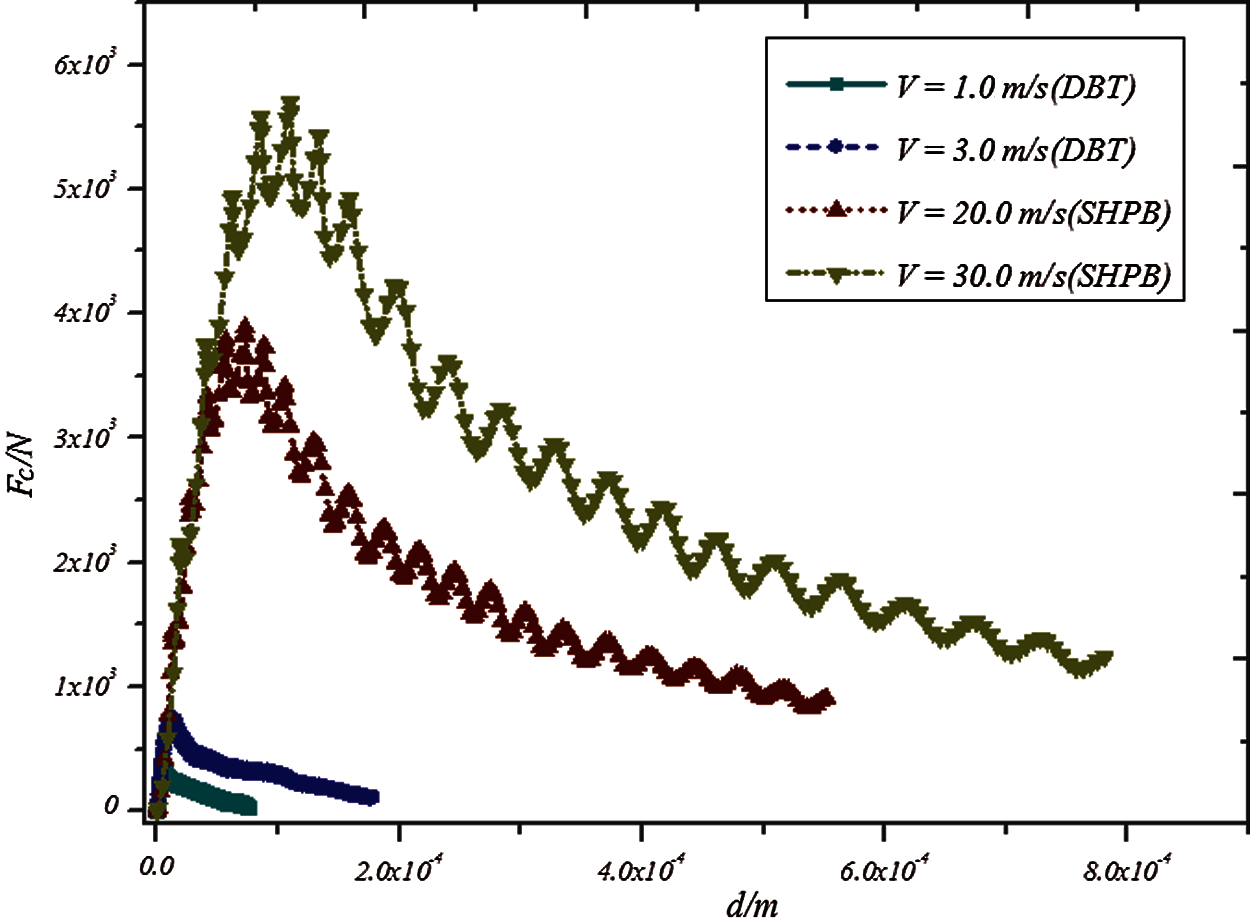
Figure 17: Curve of contact force vs. indentation depth at different impact speeds

Figure 18: Damage of glass specimens at different times

5  Conclusion

This paper proposes a new contact damage model of brittle materials based on ordinary state-based peridynamic theory by introducing the contact force function. The simulation results of the Hertzian contact (nonembedded contact) problem show that the embedded distance de gradually approaches zero (the assumption of no embedding is satisfied), and contact force Fc gradually approaches the theoretical solution with the increase in contact modulus cn. Therefore, for nonembedded contact problems, the value of the contact modulus cn should be as large as possible to satisfying the computer truncation error and the stability requirements of differential solution. The calculation error of the contact force decreases with the decrease in relative discrete size. The smaller the relative discrete size (the more discrete material points), the more time consuming the calculation. When the relative discrete size is less than a certain critical value, the effect of improving the error is unremarkable. The penalty-based method of peridynamics can be used to simulate the contact problem well by selecting the appropriate relative discrete size and the contact modulus. The low loading rate of DBT and high loading rate of SHPB are considered to simulate the failure process of glass specimen under impact load. For low loading rate, the final damage form is mainly a small amount of fragments. For the high-speed impact of SHPB, the sample appears to be broken. The simulation results are in good agreement with the test results.

The proposed damage contact model of peridynamics has a good application prospect and can be extended to the simulation of other similar materials, such as the impact fracture process of ice. The calculation model can be enriched and developed. The contact force only considers the vertical force. If the horizontal friction force is considered simultaneously, the response and failure mechanism of typical brittle materials under impact load can be better analyzed.

Acknowledgement: This research is financially by the National Natural Science Foundation of China (Nos. 11932006, U1934206, 12002118). And The Natural Science Foundation of the Jiangsu Higher Education Institutions of China (No. 20KJB580015). The snapshots were performed using the visualisation tool Ensight.

Funding Statement: This study was funded by National Natural Science Foundation of China (Nos. 11932006, U1934206), Recipient: Qing Zhang. And National Natural Science Foundation of China (No. 12002118), Recipient: Xin Gu. And Natural Science Foundation of the Jiangsu Higher Education Institutions of China (No. 20KJB580015). Recipient: Runpu Li.

Conflicts of Interest: The authors claim that none of the material in the paper has been published or is under consideration for publication elsewhere. The publication has been approved by all co-authors. We have no conflict of interest to declare, All data generated or analysed during this study are included in this published article.

Appendix A.

The Herzian contact of the rigid body is considered in Fig. A-1, and the contact stress of the sphere can be expressed as

P=P01−r2a2 (A1)

where r=x2+y2+z2.

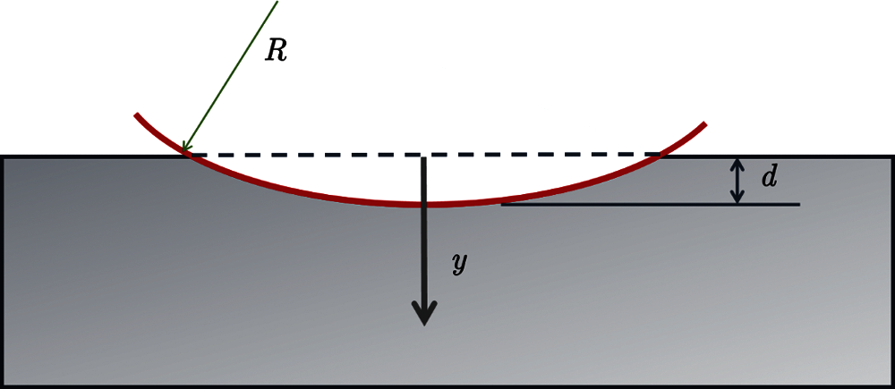
Figure A-1: Herzian contact problem of Rigid body

For a semi-infinite elastic body, the elastic mechanics solution of the concentrated force Fy is [46]

uy=1+ν2πE[2(1−ν)r+y2r3]Fy (A2)

When the contact surface y=0,

uy=1−ν2πErFy (A3)

Then, when the distributed force is considered

uy=1−ν2πE∬P(x′,z′)dx′dz′r (A4)

where r=(x−x′)2+(z−z′)2. Substituting the above Eq. (A2) into the Eq. (A4),

Fy=∬P(x,z)dxdz (A5)

And

uy=d−r2R (A6)

where d is the indentation depth, R is the radius of the sphere. The relationship between contact force and indentation depth is

Fy=4E3(1−ν2)Rd3 (A7)

This work is licensed under a Creative Commons Attribution 4.0 International License, which permits unrestricted use, distribution, and reproduction in any medium, provided the original work is properly cited.