| Computer Modeling in Engineering & Sciences |
DOI: 10.32604/cmes.2021.015375
ARTICLE
Fractional Analysis of Dynamical Novel COVID-19 by Semi-Analytical Technique
1School of Systems and Technology, University of Management and Technology, Lahore, 54770, Pakistan
2Department of Mathematics, Cankaya University, Ankara, 06530, Turkey
3Institute of Space Sciences, Magurele, Bucharest, 077125, Romania
4Department of Mathematics, Govt. College Township, Punjab Higher Education Department, Lahore, 54770, Pakistan
5Department of Mathematics, Islamia University of Bahawalpur, Bahawalpur, 63100, Pakistan
6Department of Mathematics, University of Management and Technology, Lahore, 54770, Pakistan
7Institute for Groundwater Studies, University of the Free State, Bloemfontein, 9300, South Africa
*Corresponding Author: M. B. Riaz. Email: bilalsehole@gmail.com
Received: 14 December 2020; Accepted: 24 June 2021
Abstract: This study employs a semi-analytical approach, called Optimal Homotopy Asymptotic Method (OHAM), to analyze a coronavirus (COVID-19) transmission model of fractional order. The proposed method employs Caputo's fractional derivatives and Reimann-Liouville fractional integral sense to solve the underlying model. To the best of our knowledge, this work presents the first application of an optimal homotopy asymptotic scheme for better estimation of the future dynamics of the COVID-19 pandemic. Our proposed fractional-order scheme for the parameterized model is based on the available number of infected cases from January 21 to January 28, 2020, in Wuhan City of China. For the considered real-time data, the basic reproduction number is R0 ≈ 2.48293 that is quite high. The proposed fractional-order scheme for solving the COVID-19 fractional-order model possesses some salient features like producing closed-form semi-analytical solutions, fast convergence and non-dependence on the discretization of the domain. Several graphical presentations have demonstrated the dynamical behaviors of subpopulations involved in the underlying fractional COVID-19 model. The successful application of the scheme presented in this work reveals new horizons of its application to several other fractional-order epidemiological models.
Keywords: Novel COVID-19; semi-analytical scheme; fractional analysis
Humans have invented many scientific methods so far and have set in motion several steps to avoid, even to cure, some of the lethal diseases. Although they believed they had conquered nature, corona-virus appeared killing thousands of people in China. Coronavirus has also been spread in many countries from Africa to Europe. Coronavirus 2019 (COVID-19) is a contagious virus causing infection to the respiratory system and is widely spread from humans to humans. The first infected case of this new COVID-19 disease was identified on December 31, 2019 in the city of Wuhan, China, the capital of Hubei province [1]. Reportedly, main symptom was development of the pneumonia without any diagnosable cause and the available therapies and vaccines were not found effective [2]. It was also noticed that the transfer of the virus among human takes place due to their mutual contact [3]. Following the spread of COVID-19 virus in Wuhan City of China, the virus was also spread to other Chinese cities rapidly. In turn, the virus was proliferated to other areas including Asia, Europe, and North America. It is known that it takes 2 to 10 days for signs to emerge. The symptoms include troubled breathing, fever and coughing. A total number of 4593 infected cases and 132 deaths were reported until January 28, 2020 and more details on the latest infections and deaths due to the virus were yet to come.
Mathematical models play a vital role not only in understanding the dynamics of infection but also in investigating the recommendable conditions under which the disease will persist or wiped out. Presently, governments and researchers have shown great concerns to COVID-19 because of high transmission rate and noteworthy disease induced death rate. The COVID-19 virus is generally transferred when an infected person releases droplets generated by sneezing, coughing or exhaling. The confirmed cases of COVID-19 have reached nearly fifty four million all around the globe, and more than 1.3 million deaths have been caused by this virus. As of November 13, 2020, according to Worldometers [4] USA, Brazil and India are the top countries with maximum death tolls amounting to 2.48, 1.64 and 1.28 million, respectively.
Keenly tracking the corona virus transmission, researchers have organized to speed up the diagnostic processes, and several types of vaccines are under investigation against COVID-19. For example, Cao et al. [5,6] studied and discussed the outcomes features of victims of COVID-19 in ICUs. Nesteruk [7] proposed a susceptible-infected-recovered (SIR) epidemic model and extracted some valuable guidelines through statistical analysis of the model parameters. An amended SIR model of COVID-19 was proposed in another study [8] to predict the exact count of infections and the additional burden on ICUs and isolation units. The count of coronavirus cases appeared higher than the number of cases predicted by February 2020. It lead to exert more emphasize on focusing the research on modernizing the corona virus predictions in the view of latest data and considering more complex mathematical models. Presently, no patent therapeutic agents or vaccines for treatment or prevention from coronavirus are available, however the research based investigations into vaccine candidates and potential antivirals are ongoing in several countries. Drug development is a comparatively shorter process as compared to development, testing and distribution of vaccine and any cure for COVID-19 is not expected to be available before 2021. The dense places are ideal environments where the virus can spread easily. It was agreed that human close contact is one of the possible causes of COVID-19 outbreaks. Therefore, the quarantine of the COVID-19 victims can lessen the threat of further disease proliferation. The important measures taken to reduce the spread of virus include small contact rate and social distancing. The impact of such measures was investigated by Zeb et al. [9] by proposing and analyzing a SEIIR (susceptible-exposed-infected-isolated-recovered) model. They concluded that the individuals infected from coronavirus infectious disease must be referred to isolated compartment at various rates. A logistic growth model of COVID-19 was studied by Batista [10] and was employed to predict the ultimate volume of the epidemic. The dynamical behavior of coronavirus has been studied by several researchers through various COVID-19 transmission models [7–11].
Over the last thirty years, fractional derivatives have captivated the numerous researchers after recognition of the fact that in comparison to the classical derivatives, fractional derivatives are more reliable operators to model the real world physical phenomenons. In dynamical problems, fractional calculus (FC) based modeling is receiving a rapid popularity nowadays. The mathematical modeling of many physical and engineering models based on the idea of FC exhibits highly precise and accurate experimental results as compared to the models based on conventional calculus. The non-integer differential operators such as Caputo, Caputo-Fabrizio and ABC are fractional operators that transform the ordinary model to generalized model. In this article, we present a novel research on a fractional order dynamical model that underpins the propagation of coronavirus infectious disease and provide some forecasting with real world data. We extend an integer-order model formulation to a fractional order model by adding the Caputo sense of fractional derivative. The reason of using the Caputo fractional derivative is that it possesses several basic characteristics of fractional calculus. Moreover, the transmission behavior described in the model can be better defined by using Caputo operator. Research based on derivatives in Caputo sense and its applications to different models emerging in various disciplines of engineering and other sciences can be observed in several past studies [12–16]. Few additional linked researches on Caputo and other fractional order derivative implementations can be found in literature [17–32]. Since the number of infected cases reported from January 21 to January 28, 2020 is comparatively higher than those of on initial days, therefore we have considered this period for the formulation of the mathematical model as a parameterized model. In Section 2, transitory details of various mathematical models showing evolution of COVID-19 from bats to humans have been provided. Section 3 presents basic properties of the fractional order COVID-19 model. The Section 4 consists of the development of a semi-analytical scheme for the solution of the considered fractional order COVID-19 model. The simulation results of the proposed scheme based upon model fitted data are presented in Section 5. In the end, some fruitful conclusions have been presented.
2 Mathematical Modeling of COVID-19 Evolution
Presuming that the transmission occurs primarily within the population of bats and afterwards the transmission occurs to wild animals usually termed as hosts. Hunting of these carriers and then their transportation to the supply markets of seafood are considered as virus reservoirs. By exposing to the market, people get the risk of infection. In the following subsections, we revisit the evolution of the COVID-19 evolutionary tracks from bats to humans in the form of three mathematical models.
2.1 Model 1: Transmission of Corona Virus-19 among Bats and Hosts Populations
From the mathematical modeling point of view, let us denote the size of entire population of bats by
The susceptible bat population is hired via birth rate
Eqs. (1)–(8) are subject to some non-negative initial conditions.
2.2 Model 2: Transmission of COVID-19 from Seafood Market to Human
Let
The governing Eqs. (9)–(14) are also subject to some initial conditions. The parameter
2.3 Model 3: Transmission of COVID-19 among Human with Reservoir
This model presents changing aspects of transmission of COVID-19 among human that are due to the close contacts of human population with the contagious environment without direct contact to virus hosts. Peoples' birth and natural death rates are denoted by the parameters
There also exist some initial conditions of this model. Considering that the rates of symptomatic and asymptomatic infections due to reservoir M are constant, we denote these constant rates by parameters
3 Dynamical Fractional Order Model of COVID-19
To develop fractional order COVID-19 model, we describe some basic definitions from fractional calculus, which play vital role in fractional calculus for solving fractional order system of differential equations. These definitions consist of fractional integral operator of a function
The integral operator of fractional order in Riemann–Liouville sense with order α ≥ 0 of
where
Replacing the time derivatives of state variables by Caputo sense fractional order derivatives in Model 3, we obtain the following generalized COVID-19 model of fractional order in Caputo sense fractional derivative operator.
Initial conditions obeyed by the model are:
By adding Eqs. (15)–(19), we obtain human population's total dynamics as under.
Integrating over
It implies that the total population has an upper bound of
The points of equilibrium of the above fractional order dynamical COVID-19 model are calculated by solving the nonlinear algebraic equations obtained by equating the fractional time derivatives in Eqs. (21)--(26) to zero. Disease free and endemic equilibrium points denoted by
where,
The solution of the polynomial equation
where,
Clearly
The essential reproduction quantity (
The spectral radius
The threshold value for

4 Optimal Homotopy Asymptotic Method (OHAM) Scheme for Fractional COVID-19 Model
Now we develop OHAM scheme for solving underlying fractional order COVID-19 model. OHAM technique is known for its rapid convergence as compared to other techniques. It produces an approximate closed form of the desired solutions and, hence, is known as semi-analytical approach. Procedure of our approximate OHAM scheme has been derived by following the relevant principles as described in literature [34,35]. The underlying COVID-19 fractional order model consists of six governing equations. In the following steps we carry out complete calculations of OHAM scheme for all equations of the model.
Step-1) Homotopies of the governing equations:
We construct the homotopy equations by defining the real valued functions
In the above relations
Step-2) The steps of OHAM scheme for finding the approximate solution have been carried out in details for the first governing Eq. (28) only. The procedure for the remaining Eqs. (29)–(33) is quite similar. We start by expanding
The convergence of above series depends upon auxiliary constants
For
Step-3) Comparing the coefficients of like powers of ‘
And so on.
Step-4) Using Reimann-Liouville sense of integral on governing equation of susceptible population and using the initial condition
where
By substituting the values from Eqs. (40)–(42) in Eq. (43), we obtain second order approximate result of Eq. (21) as:
Adopting the same procedure presented in Steps 1–4, we find the following approximate solutions for the state variables
Step-5) In this step, the values of auxiliary constants
The minimization process of each
This section is dedicated for presentation of the closed form semi-analytical solutions for all of the state variables and demonstration of their dynamics through graphical exhibition of related simulation results. Model 4 has total six equations. That means COVID-19 fractional model is to analyzed by observing the behaviors of six subpopulations
The considered values for model parameters are presented by Tab. 1. All figures in the following cases describe the individual behavior of model subpopulations for various values of α. The evolution time
5.1 Dynamics of Susceptible Human Population
For the fractional analysis of human susceptible population we calculate the auxiliary constants (
where, the residual, of susceptible population, denoted by
Imposing the necessary conditions for minimum residual, we can find
Tab. 2 presents the optimized values of auxiliary constants of the second order approximate solution for susceptible population considering various orders of fractional derivative. The corresponding second order approximate solution for
5.2 Dynamics of Exposed Population
The auxiliary constants (
where, the residual of exposed population, denoted by
Imposing the necessary conditions for minimum residual, we can find
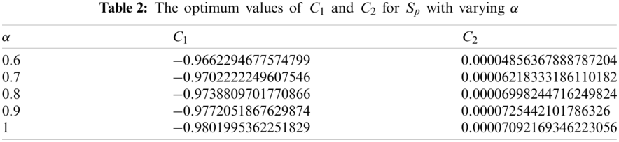
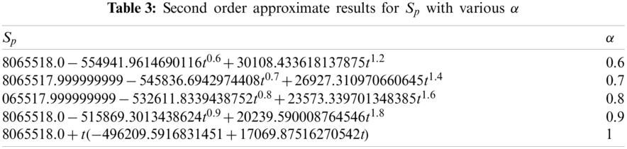
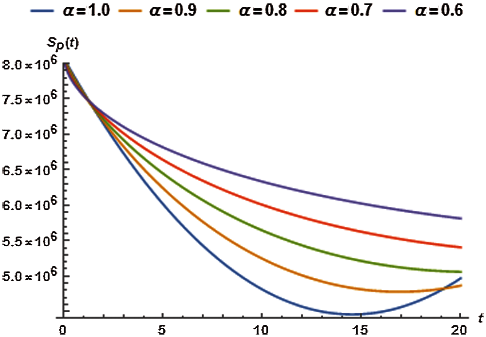
Figure 1: Susceptible population vs. time t
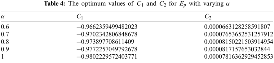
Considering various orders of the fractional derivative, above necessary conditions provide the relevant optimum values of auxiliary constants for the exposed population and are presented in Tab. 4.
The OHAM scheme based second order solution for the exposed population
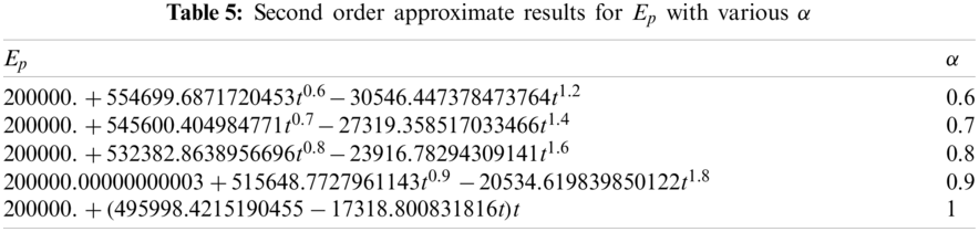
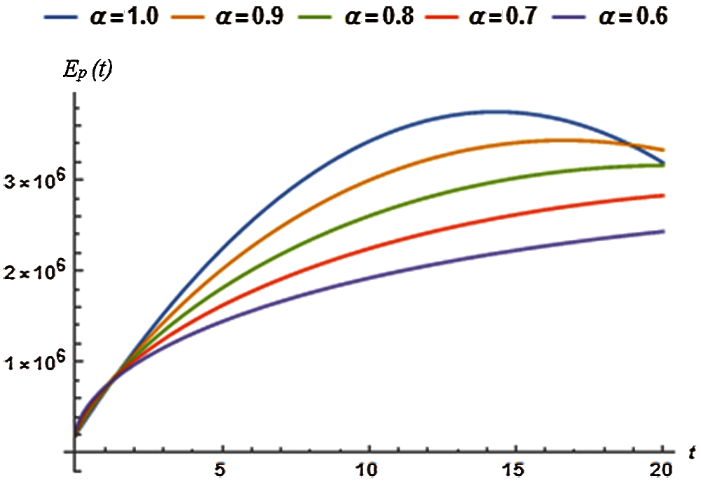
Figure 2: Exposed population vs. time t
5.3 Dynamics of Infected (Symptomatic) Population
The values of auxiliary constant
where, the residual of infected (symptomatic) population, denoted by
Solving the following equations for
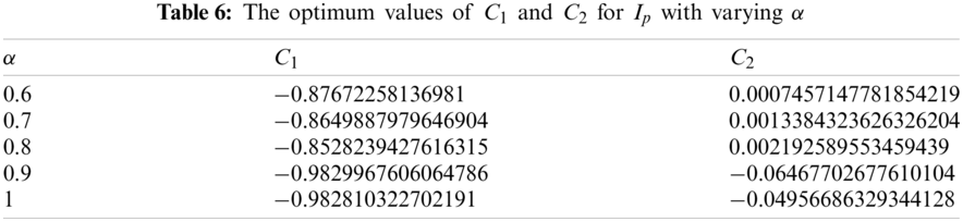
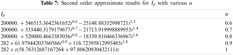
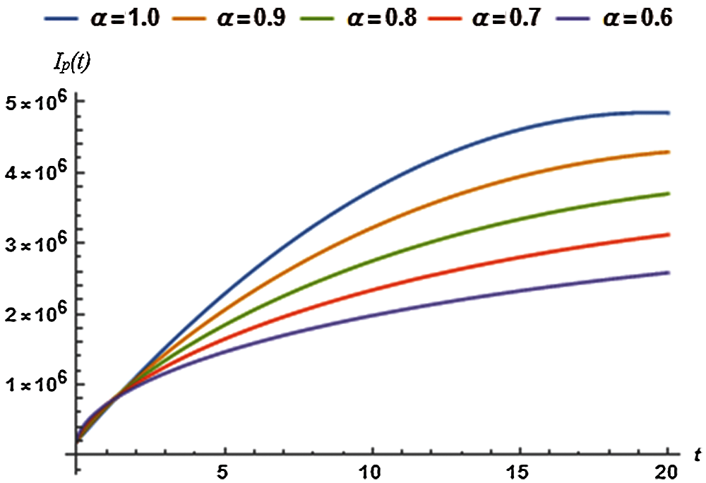
Figure 3: Infected population vs. time t
5.4 Dynamics of Asymptotically Infected Population
The values of auxiliary constant
where, the residual of asymptotically infected population, denoted by
The values of
Tab. 9 displays the second order solution for
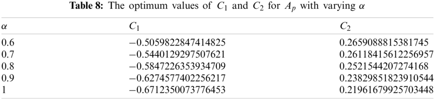
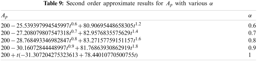
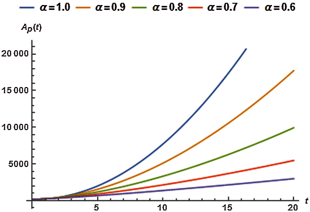
Figure 4: Asymptomatically infected population vs. time t
5.5 Dynamics of the Recovered or the Removed Population
The following total error function corresponding to recovered population is obtained from Eq. (48):
The residual
Solving the following necessary conditions we obtain the values of
The closed form solution for recovered population is presented in Tab. 11 using different values of α and the relevant graphs are exhibited in Fig. 5.
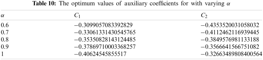
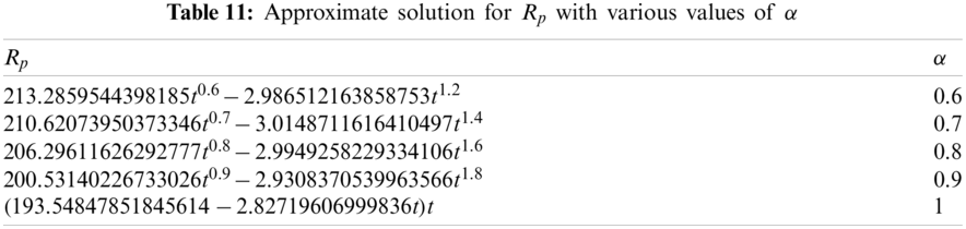
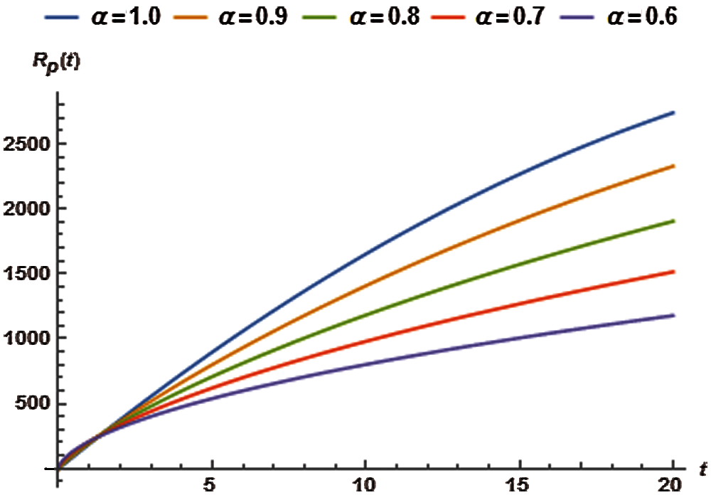
Figure 5: Recovered population vs. time t
5.6 Dynamics of the Reservoir Compartment
Applying the least square approach for the auxiliary constant of Eq. (49) we get following total error function:
The residual
The solutions of following equations give the values of
The approximate solutions for M have been presented in Tab. 13 whereas the impact of variation in order of the fractional derivative has been shown in Fig. 6.
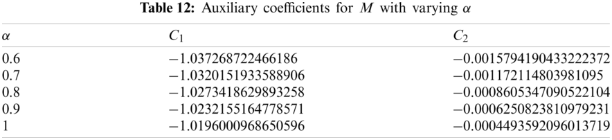
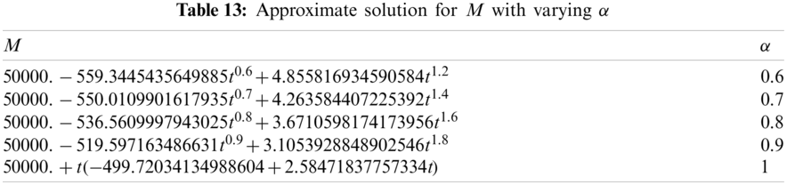
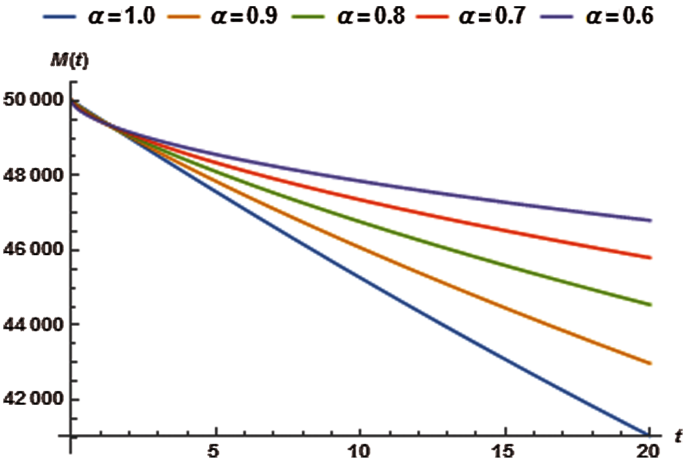
Figure 6: Reservoir saturation vs. time t
In this study, closed form semi-analytical approximate solution has been presented for fractional order COVID-19 model in Caputo sense of derivative operator. The underlying model involves parameters that were extracted by fitting real data into the dynamical model. The fitted parameters are responsible for a high reproduction number
Acknowledgement: The authors are thankful to their respective departments and Universities.
Funding Statement:The authors received no specific funding for this study.
Conflicts of Interest:The authors declare that they have no conflicts of interest to report regarding the present study.
1. Macrotrends (2020). Wuhan, China Population 1950–2020. http://www.macrotrends.net/cities/20712/wuhan/population. [Google Scholar]
2. The New York Times (2020). Is the World Ready for the Coronavirus? https://www.cnbc.com/2020/01/24/chinas-hubei-province-confirms-15-more-deaths-due-to-coronavirus.html. [Google Scholar]
3. CNBC (2020). China Virus Death Toll Rises to 41, More than 1,300 Infected Worldwide. https://www.cnbc.com/2020/01/24/chinas-hubei-province-confirms-15-more-deaths-due-to-coronavirus.html. [Google Scholar]
4. COVID-19 Coronavirus updates (2020). https://www.worldometers.info/coronavirus/. [Google Scholar]
5. Cao, J. L., Tu, W. J., Hu, X. R., Liu, Q. (2020). Clinical features and short-term outcomes of 102 patients with coronavirus disease 2019 in Wuhan, China. Clinical Infectious Diseases, 71(15), 748–755. DOI 10.1093/cid/ciaa243. [Google Scholar] [CrossRef]
6. Cao, J. L., Hu, X. R., Tu, W. J., Liu, Q. (2020). Clinical features and short-term outcomes of 18 patients with corona virus disease 2019 in intensive care unit. Intensive Care Medicine, 46(5), 851–853. DOI 10.1007/s00134-020-05987-7. [Google Scholar] [CrossRef]
7. Nesteruk, I. (2020). Statistics-based predictions of coronavirus epidemic spreading in mainland China. Innovative Biosystems and Bioengineering, 4(1), 13–18. DOI 10.20535/ibb.2020.4.1.195074. [Google Scholar] [CrossRef]
8. Ming, W., Huang, J. V., Zhang, C. J. P. (2020). Breaking down of the healthcare system: Mathematical modelling for controlling the novel coronavirus (2019-nCoV) outbreak in Wuhan, China. bioRxiv. DOI 10.20535/ibb.2020.4.1.195074. [Google Scholar] [CrossRef]
9. Zeb, A., Alzahrani, E., Erturk, V. S., Zaman, G. (2020). Mathematical model for coronavirus disease 2019 (COVID-19) containing isolation class. BioMed Research International, 2020, 7. DOI 10.1155/2020/3452402. [Google Scholar] [CrossRef]
10. Batista, M. (2020). Estimation of the final size of the coronavirus epidemic by SIR model. https://www.researchgate.net/publication/339311383. [Google Scholar]
11. Victor, A. (2020). Mathematical predictions for COVID-19 as a global pandemic. DOI 10.2139/ssrn.3555879. [Google Scholar] [CrossRef]
12. Sarwar, S., Zahid, M. A., Iqbal, S. (2016). Mathematical study of fractional-order biological population model using optimal homotopy asymptotic method. International Journal of Biomathematics, 9(6), 1650081. DOI 10.1142/S1793524516500819. [Google Scholar] [CrossRef]
13. Sarwar, S., Iqbal, S. (2017). Stability analysis, dynamical behavior and analytical solutions of nonlinear fractional differential system arising in chemical reaction. Chinese Journal of Physics, 56(1), 374–384. DOI 10.1016/j.cjph.2017.11.009. [Google Scholar] [CrossRef]
14. Iqbal, S., Mufti, M. R., Afzal, H., Sarwar, S. (2019). Semi analytical solutions for fractional order singular partial differential equations with variable coefficients. AIP Conference Proceedings, 2116(1), 3000071–3000074. DOI 10.1063/1.5114307. [Google Scholar] [CrossRef]
15. Sarwar, S., Iqbal, S. (2017). Exact solutions of the non-linear fractional klein-gordon equation using the optimal homotopy asymptotic method. Nonlinear Science Letters A, 8(4), 340–348. [Google Scholar]
16. Sarwar, S., Alkhalaf, S., Iqbal, S., Zahid, M. A. (2015). A note on optimal homotopy asymptotic method for the solutions of fractional order heat and wave-like partial differential equations. Computers & Mathematics with Applications, 7(5), 942–953. DOI 10.1016/j.camwa.2015.06.017. [Google Scholar] [CrossRef]
17. Friehet, A., Hasan, S., Al-Smadi, M., Gaith, M., Momani, S. (2019). Construction of fractional power series solutions to fractional stiff system using residual functions algorithm. Advances in Difference Equations, 2019, 95. DOI 10.1186/s13662-019-2042-3. [Google Scholar] [CrossRef]
18. Oldham, K. B., Spanier, J. (1974). The fractional calculus. New York, USA: Academic Press. [Google Scholar]
19. Miller, K. S., Ross, B. (1993). An introduction to the fractional calculus and fractional differential equations. New York, USA: Wiley-Interscience. [Google Scholar]
20. Podlubny, I. (1999). Fractional differential equations. New York, USA: Academic Press. [Google Scholar]
21. Younas, H. M., Mustahsan, M., Manzoor, T., Salamat, N., Iqbal, S. (2019). Dynamical study of fokker-Planck equations by using optimal homotopy asymptotic method. Mathematics, 7(3), 264. DOI 10.3390/math7030264. [Google Scholar] [CrossRef]
22. Mustahsan, M., Younas, H. M., Iqbal, S., Nisar, K. S., Singh, J. (2020). An efficient analytical technique for time-fractional parabolic partial differential equations. Frontiers in Physics, 8, 131. DOI 10.3389/fphy.2020.00131. [Google Scholar] [CrossRef]
23. Blake, T. D., Ruschak, K. J., Kistler, S. F., Schweizer, P. M. (1997). Liquid film coating. London, UK: Chapman & Hall. [Google Scholar]
24. Kumar, S., Atangana, A. (2020). A numerical study of the nonlinear fractional mathematical model of tumor cells in presence of chemotherapeutic treatment. International Journal of Biomathematics, 13(3), 2050021. DOI 10.1142/S1793524520500217. [Google Scholar] [CrossRef]
25. Pandey, P., Kumar, S., Das, S. (2019). Approximate analytical solution of coupled fractional order reaction-advection-diffusion equations. The European Physical Journal Plus, 134(7), 364. DOI 10.1140/epjp/i2019-12727-6. [Google Scholar] [CrossRef]
26. Kumar, S. (2020). Numerical solution of fuzzy fractional diffusion equation by chebyshev spectral method. Numerical Methods for Partial Differential Equations, 2020, 1–19. DOI 10.1002/num.22650. [Google Scholar] [CrossRef]
27. Kumar, S., Gómez Aguilar, J. F., Pandey, P. (2020). Numerical solutions for the reaction-diffusion, diffusion-wave and cattaneo equations using a new operational matrix for the caputo-fabrizio derivative. Mathematical Methods in the Applied Sciences, 43(15), 8595–8607. DOI 10.1002/mma.6517. [Google Scholar] [CrossRef]
28. Kumar, S., Pandey, P., Das, S. (2020). Operational matrix method for solving nonlinear space-time fractional order reaction-diffusion equation based on genocchi polynomial. Special Topics & Reviews in Porous Media: an International Journal, 11(1), 33–47. DOI 10.1615/SpecialTopicsRevPorousMedia.2020030750. [Google Scholar] [CrossRef]
29. Kumar, S., Pandey, P. (2020). Quasi wavelet numerical approach of non-linear reaction diffusion and integro reaction-diffusion equation with atangana–Baleanu time fractional derivative. Chaos, Solitons & Fractals, 130, 109456. DOI 10.1016/j.chaos.2019.109456. [Google Scholar] [CrossRef]
30. Kumar, S., Cao, J., Abdel-Aty, M. (2020). A novel mathematical approach of COVID-19 with non-singular fractional derivative. Chaos, Solitons & Fractals, 139, 110048. DOI 10.1016/j.chaos.2020.110048. [Google Scholar] [CrossRef]
31. Pandey, P., Kumar, S., Jafari, H., Das, S. (2019). An operational matrix for solving time-fractional order cahn-hilliard equation. Thermal Science, 23, 369–369. DOI 10.2298/TSCI190725369P. [Google Scholar] [CrossRef]
32. Ali, Z., Rabiei, F., Shah, K., Khodadadi, T. (2020). Modeling and analysis of novel COVID-19 under fractal-fractional derivative with case study of Malaysia. Fractals, 29(1). DOI 10.1142/S0218348X21500201. [Google Scholar] [CrossRef]
33. Ali, Z., Rabiei, F., Shah, K., Khodadadi, T. (2020). Qualitative analysis of fractal-fractional order COVID-19 mathematical model with case study of wuhan. Alexandria Engineering Journal, 60(1), 477–489. DOI 10.1016/j.aej.2020.09.020. [Google Scholar] [CrossRef]
34. Iqbal, S., Idrees, M., Siddiqui, A. M., Ansari, A. R. (2010). Some solutions of linear and nonlinear klein-gordon equations using the optimal homotopy asymptotic method. Applied Mathematics and Computation, 216(10), 2898–2909. DOI 10.1016/j.amc.2010.04.001. [Google Scholar] [CrossRef]
35. Iqbal, S., Javed, A. (2011). Application of optimal homotopy asymptotic method for the analytic solution of singular lane-emden type equation. Applied Mathematics and Computation, 217(9), 7753–7761. DOI 10.1016/j.amc.2011.02.083. [Google Scholar] [CrossRef]
36. Ruschak, K. J. (1985). Coating flows. Annual Review of Fluid Mechanics, 17, 65–89. DOI 10.1146/annurev.fluid.36.050802.122049. [Google Scholar] [CrossRef]
37. Gaskell, P. H., Savage, M. D., Summers, J. L. (1995). The mechanics of thin film coatings. Proceedings of the First European Coating Symposium, pp. 19–22. Leeds University, Leeds, UK. [Google Scholar]
 | This work is licensed under a Creative Commons Attribution 4.0 International License, which permits unrestricted use, distribution, and reproduction in any medium, provided the original work is properly cited. |