| Computer Modeling in Engineering & Sciences |
DOI: 10.32604/cmes.2021.016431
ARTICLE
Determinantal Expressions and Recursive Relations for the Bessel Zeta Function and for a Sequence Originating from a Series Expansion of the Power of Modified Bessel Function of the First Kind
1College of Mathematics and Physics, Inner Mongolia University for Nationalities, Tongliao, 028043, China
2School of Mathematics and Informatics, Henan Polytechnic University, Jiaozuo, 454003, China
3School of Mathematical Sciences, Tiangong University, Tianjin, 300387, China
*Corresponding Author: Bai-Ni Guo. Email: bai.ni.guo@gmail.com Dedicated to Professor Dr. Mourad E. H. Ismail at University of Central Florida in USA
Received: 05 March 2021; Accepted: 07 June 2021
Abstract: In the paper, by virtue of a general formula for any derivative of the ratio of two differentiable functions, with the aid of a recursive property of the Hessenberg determinants, the authors establish determinantal expressions and recursive relations for the Bessel zeta function and for a sequence originating from a series expansion of the power of modified Bessel function of the first kind.
Keywords: Determinantal representation; recursive relation; series expansion; first kind modified Bessel function; Bessel zeta function; Pochhammer symbol; gamma function; Hessenberg determinant
1 Introduction and Motivations
Recall from [1], and [2,3] that the classical Euler gamma function
Recall from [4], that the modified Bessel function of the first kind
where
Concretely and explicitly, the power series expansion
was listed [5], For
where
and
with the convention that the sum is zero if the starting index exceeds the finishing index. By the way, in the paper [6], there are new conclusions and applications on series expansions of powers of several fundamental elementary functions. In [5], the first five expressions for Bk(
In [7], the recursive relation (3) was simplified as
in which the sequence bk(
In [8], Theorem 2.3, alternative recursive relations
and
were derived via a probabilistic interpretation of the series expansion of powers of a general series.
In [9], the complete Bell polynomials, denoted by
By the way, in the article [10], some new results on the Bell polynomials of the second kind are surveyed and reviewed. Let
where
for q > 1 was originally introduced and studied in [11–14]. In [8], there are the following special values:
Theorems 3.1 and 3.2 in [8] read that
and
Corollary 4.2 in [8] confirms that Bk(
One of the reasons why ones investigated the series expansion (2) and the sequence Bk(
In the papers [8,18] and in Entry A131490 of The On-Line Encyclopedia of Integer Sequences, the sequence bk+1(
Theorem 5.1 in [8] reads that
Corollary 5.2 in [8] asserts that the number bk+1(0) is an integer. Theorem 5.4 in [8] reads that
and confirms that, due to the second value in (7), the sequence bk(
In this paper, we will establish determinantal expressions and recursive relations of the sequences bk+1(
2 Determinantal Representations via Ratios of Gamma Functions
We are now in a position to establish determinantal expressions of the sequences bk+1(
Theorem 2.1. For
where
with ( −1)!! = 1 is a (2k + 1)
is a
Proof. Replacing
This implies that
and
for
Hence, we obtain
Let
and
Then
and
as
In [19], there exists a general formula
for
Accordingly, we acquire
which can be rearranged as the form in (9). The proof of Theorem 2.1 is complete.
Theorem 2.2. For
where
and
with ( −1)!! = 1 and the convention
Proof. This can be deduced from taking
Theorem 2.3. For
where the matrices P2k+1, 1(
Proof. Combining (8) with (9) in Theorem 2.1 results in
Further simplifying gives (15). The proof of Theorem 2.3 is complete.
3 Determinantal Representations via the Pochhammer Symbols
For
In terms of the Pochhammer symbol (z)n defined by (16), we can rewrite Theorems 2.1–2.3 for intuitive and visual beauty respectively as follows:
Theorem 3.1. For
Proof. In the proof of Theorem 2.1, we can write
Substituting this equation into (12) and considering the definition in (16) lead to (17). The proof of Theorem 3.1 is complete.
Theorem 3.2. For
where ( −1)!! = 1.
Proof. This can be deduced from letting
Theorem 3.3. For
Proof. Combining (8) with (17) in Theorem 3.1 results in
Further simplifying gives (19). The proof of Theorem 3.3 is complete.
In this section, we establish recursive relations of the sequences bk+1(
Theorem 4.1. For
Consequently, the sequence ( −1)k+12
Proof. Let D0 = 1 and
for
for n
for 1
for 1
for
for
which can be simplified as (20).
Substituting (8) into (20) produces
which can be rearranged as
The recursive relation (21) is thus proved. The proof of Theorem 4.1 is complete.
5 More Numerical Computation of the First Few Values
Via newly-established determinantal expressions (9), (14), (15), (17)–(19), with the aid of the famous software Mathematica version 12.0, we numerically compute more special values of the sequences bk+1(
We notice that the numerical computation of
Using the famous software Mathematica version 12.0, we plotted graphs of
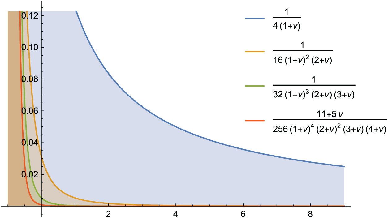
Figure 1: Graphs of
In this paper, by virtue of a general formula (13) for derivatives of the ratio of two differentiable functions and with the aid of a recursive property (23) of the Hessenberg determinants (22), we establish six determinantal expressions (9), (14), (15), (17)–(19), find two recursive relations (20) and (21) for the sequence bk+1(
Acknowledgement: The authors thank 1. Jiaying Chen and Geng Li (Undergraduates Enrolled in 2018 at School of Mathematical Sciences, Tianjin Polytechnic University, China), for their valuable help downloading the papers [5,8,17] on 27 January 2021. 2. Christophe Vignat (Universite d’Orsay, France; Tulane University, USA; cvignat@tulane.edu) for his sending electronic version of the paper [8] on 28 January 2021. 3. Anonymous referees for their careful reading of, helpful suggestions to, and valuable comments on the original version of this paper.
Funding Statement: The first author, Mrs. Yan Hong, was partially supported by the Natural Science Foundation of Inner Mongolia (Grant No. 2019MS01007), by the Science Research Fund of Inner Mongolia University for Nationalities (Grant No. NMDBY15019), and by the Foundation of the Research Program of Science and Technology at Universities of Inner Mongolia Autonomous Region (Grant Nos. NJZY19157 and NJZY20119) in China.
Conflicts of Interest: The authors declare that they have no conflicts of interest to report regarding the present study.
1. Temme, N. M. (1996). Special functions: An introduction to classical functions of mathematical physics. New York: A Wiley-Interscience Publication, John Wiley & Sons, Inc. DOI 10.1002/9781118032572. [Google Scholar] [CrossRef]
2. Qi, F., Guo, B. N. (2021). From inequalities involving exponential functions and sums to logarithmically complete monotonicity of ratios of gamma functions. Journal of Mathematical Analysis and Applications, 493(1), 19. DOI 10.1016/j.jmaa.2020.124478. [Google Scholar] [CrossRef]
3. Qi, F., Li, W. H., Yu, S. B., Du, X. Y., Guo, B. N. (2021). A ratio of finitely many gamma functions and its properties with applications. Revista de la Real Academia de Ciencias Exactas, Físicas y Naturales Serie A Matemáticas, 115(2), 14. DOI 10.1007/s13398-020-00988-z. [Google Scholar] [CrossRef]
4. Abramowitz, M., Stegun, I. A. (1972). Handbook of mathematical functions with formulas, graphs, and mathematical tables. National bureau of standards, applied mathematics series, vol. 55. Mineola, New York: Dover Publications. [Google Scholar]
5. Bender, C. M., Brody, D. C., Meister, B. K. (2003). On powers of Bessel functions. Journal of Mathematical Physics, 44(1), 309–314. DOI 10.1063/1.1526940. [Google Scholar] [CrossRef]
6. Guo, B. N., Lim, D., Qi, F. (2021). Series expansions of powers of arcsine, closed forms for special values of Bell polynomials, and series representations of generalized logsine functions. AIMS Mathematics, 6(7), 7494–7517. DOI 10.3934/math.2021438. [Google Scholar] [CrossRef]
7. Baricz, Á. (2010). Powers of modified Bessel functions of the first kind. Applied Mathematics Letters, 23(6), 722–724. DOI 10.1016/j.aml.2010.02.015. [Google Scholar] [CrossRef]
8. Moll, V. H., Vignat, C. (2014). On polynomials connected to powers of Bessel functions. International Journal of Number Theory, 10(5), 1245–1257. DOI 10.1142/S1793042114500249. [Google Scholar] [CrossRef]
9. Comtet, L. (1974). Advanced combinatorics: The art of finite and infinite expansions, Revised and Enlarged Edition. Dordrecht, Netherlands: Reidel Publishing Co. DOI 10.1007/978-94-010-2196-8. [Google Scholar] [CrossRef]
10. Qi, F., Niu, D. W., Lim, D., Yao, Y. H. (2020). Special values of the Bell polynomials of the second kind for some sequences and functions. Journal of Mathematical Analysis and Applications, 491(2), 31. DOI 10.1016/j.jmaa.2020.124382. [Google Scholar] [CrossRef]
11. Kishore, N. (1964). The Rayleigh polynomial. Proceedings of the American Mathematical Society, 15(6), 911–917. DOI 10.1090/S0002-9939-1964-0168823-2. [Google Scholar] [CrossRef]
12. Kishore, N. (1964). A structure of the Rayleigh polynomial. Duke Mathematical Journal, 31(3), 513–518. DOI 10.1215/S0012-7094-64-03150-3. [Google Scholar] [CrossRef]
13. Kishore, N. (1965). Binary property of the Rayleigh polynomial. Duke Mathematical Journal, 32(3), 429–435. DOI 10.1215/S0012-7094-65-03243-6. [Google Scholar] [CrossRef]
14. Kishore, N. (1968). Congruence properties of the Rayleigh functions and polynomials. Duke Mathematical Journal, 35, 557–562. DOI 10.1215/S0012-7094-68-03557-6. [Google Scholar] [CrossRef]
15. Bakker, M., Temme, N. M. (1984). Sum rule for products of Bessel functions: Comments on a paper by Newberger. Journal of Mathematical Physics, 25(5), 1266–1267. DOI 10.1063/1.526282. [Google Scholar] [CrossRef]
16. Newberger, B. S. (1983). Erratum: New sum rule for products of Bessel functions with application to plasma physics. Journal of Mathematical Physics, 24(8), 2250. 10.1063/1.525940. [Google Scholar] [CrossRef]
17. Newberger, B. S. (1982). New sum rule for products of Bessel functions with application to plasma physics. Journal of Mathematical Physics, 23(7), 1278–1281. DOI 10.1063/1.525510. [Google Scholar] [CrossRef]
18. Howard, F. T. (1985). Integers related to the Bessel function J1(z). Fibonacci Quarterly, 23(3), 249–257. [Google Scholar]
19. Bourbaki, N. (2004). Elements of mathematics: Functions of a real variable: Elementary theory, translated from the 1976 french original by Philip Spain. Elements of mathematics (Berlin). Berlin: Springer-Verlag. DOI 10.1007/978-3-642-59315-4. [Google Scholar] [CrossRef]
20. Qi, F., Huang, C. J. (2020). Computing sums in terms of beta, polygamma, and Gauss hypergeometric functions. Revista de la Real Academia de Ciencias Exactas, Físicas y Naturales Serie A Matemáticas, 114(1), 191. DOI 10.1007/s13398-020-00927-y. [Google Scholar] [CrossRef]
21. Qi, F., Kouba, O., Kaddoura, I. (2020). Computation of several Hessenberg determinants. Mathematica Slovaca, 70(6), 1521–1537. DOI 10.1515/ms-2017-0445. [Google Scholar] [CrossRef]
22. Qi, F., Niu, D. W., Lim, D., Guo, B. N. (2020). Closed formulas and identities for the Bell polynomials and falling factorials. Contributions to Discrete Mathematics, 15(1), 163–174. DOI 10.11575/cdm.v15i1.68111. [Google Scholar] [CrossRef]
23. Cahill, N. D., D’Errico, J. R., Narayan, D. A., Narayan, J. Y. (2002). Fibonacci determinants. The College Mathematics Journal, 33(3), 221–225. DOI 10.1080/07468342.2002.11921945. [Google Scholar] [CrossRef]
 | This work is licensed under a Creative Commons Attribution 4.0 International License, which permits unrestricted use, distribution, and reproduction in any medium, provided the original work is properly cited. |