Computer Modeling in Engineering & Sciences

DOI: 10.32604/cmes.2021.016917

ARTICLE

Study of Degenerate Poly-Bernoulli Polynomials by λ-Umbral Calculus

Lee-Chae Jang1, Dae San Kim2, Hanyoung Kim3, Taekyun Kim3,* and Hyunseok Lee3

1Graduate School of Education, Konkuk University, Seoul, 143-701, Korea
2Department of Mathematics, Sogang University, Seoul, 121-742, Korea
3Department of Mathematics, Kwangwoon University, Seoul, 139-701, Korea
*Corresponding Author: Taekyun Kim. Email: tkkim@kw.ac.kr
Received: 09 April 2021; Accepted: 13 May 2021

1  Introduction

Carlitz investigated the degenerate Bernoulli and Euler polynomials and numbers in [1,2], as degenerate versions of the ordinary Bernoulli and Euler polynomials and numbers. In recent years, studying degenerate versions of some special numbers and polynomials has received increased attention by mathematicians with their interests not only in combinatorial and arithmetic properties but also in applications to differential equations, identities of symmetry and probability theory (see [3–9] and references therein). Quite a few different methods have been employed in investigating degenerate versions of special numbers and polynomials, which include combinatorial methods, generating functions, umbral calculus techniques, p-adic analysis, differential equations, special functions, probability theory and analytic number theory.

Gian-Carlo Rota laid a completely rigorous foundation for umbral calculus in the 1970s, which had been in a state of manipulating sequences by a symbolic technique. The Rota’s theory is based on the modern concepts like linear functionals and differential operators. In addition, the central position in the theory is occupied by the Sheffer sequences whose generating functions are given in terms of the usual exponential function (see [10–12]). Thus one may say that umbral calculus is the study of Sheffer sequences. The impetus for [4] started from the simple question, what if the usual exponential function is replaced by the degenerate exponential functions in (1). This question arises very naturally in light of the regained recent interests in degenerate special numbers and polynomials. As it turns out, it amounts to replacing the linear functionals by the family of λ-linear functionals in (11), and the differential operators by the family of λ-differential operators in (12). Furthermore, these replacements led to define λ-Sheffer sequences which are charactered by the desired generating functions in (18). Hence one may say that λ-umbral calculus is the study of λ-Sheffer sequences.

The motivation of the present research is to demonstrate its usefulness of the newly developed λ-umbral calculus in studying some degenerate special numbers and polynomials. Recently, degenerate polyexponential functions were introduced (see [13,14]) and degenerate poly-Bernoulli polynomials were defined by means of the degenerate polyexponential functions (see (2), (10)), and some properties of the degenerate poly-Bernoulli polynomials were investigated (see [8]). The aim of this paper is to further examine the degenerate poly-Bernoulli polynomials using the above-mentioned λ-linear functionals and λ-differential operators. In more detail, these polynomials are investigated by three different tools, namely a formula about representing a λ-Sheffer sequence by another (see (20)), a formula obtained from the generating functions of λ-Sheffer sequences (see Theorem 1) and a formula arising from the definitions for λ-Sheffer sequences (see Theorems 6, 8). Then, among other things, we represent the degenerate poly-Bernoulli polynomials by Carlitz Bernoulli polynomials and degenerate Stirling numbers of the first kind, by fully degenerate Bell polynomials and degenerate Stirling numbers of the first kind, and by higher-order degenerate Bernoulli polynomials and degenerate Stirling numbers of the second kind.

The rest of this section is devoted to recalling the necessary facts that are needed throughout the paper, which includes very brief review on λ-umbral calculus.

For any λ∈ℝ, the degenerate exponential functions are defined by

eλx(t)=∑n=0∞(x)n,λtnn!,eλ(t)=eλ1(t),see[3–9],(1)

where (x)0,λ=1,(x)n,λ=x(x-λ)…(x-(n-1)λ), (n≥1). Note that limλ→0eλx(t)=ext.

The degenerate polyexponential functions are defined by Kim-Kim as

Eik,λ(x)=∑n=1∞(1)n,λxn(n-1)!nk,(k∈ℤ,|x|<1),see[7].(2)

From (1) and (2), we note that Ei1,λ(x)=eλ(x)-1.

Here we note that the polyexponential function was first considered by Hardy in [15,16], which are given by

Also, a slightly different special case of Hardy’s polyexponential function is considered, which is given by

Note that xe(x,1∣k)=Eik(x). Let logλ(t) be the compositional inverse function of eλ(t). Then we have

logλ(1+t)=∑n=1∞λn-1(1)n,1/λn!tn,see [5].(3)

Note that limλ→0 logλ(1+t)= log(1+t). Kim-Kim considered the degenerate Stirling numbers of the second kind S2,λ(n,k),(n,k≥0), which are given by

(x)n,λ=∑k=0nS2,λ(n,k)(x)k,(n≥0),see [5].(4)

As the inversion formula of (4), they also considered the degenerate Stirling numbers of the first kind given by

(x)n=∑k=0nS1,λ(n,k)(x)k,λ,(n≥0),see [5].(5)

From (4) and (5), we can derive the following equations:

1k!(eλ(t)-1)k=∑n=k∞S2,λ(n,k)tnn!,see [4–6],(6)

and

1k!(logλ(1+t))k=∑n=k∞S1,λ(n,k)tnn!,see [4, 5, 8].(7)

For r∈ℕ, Carlitz introduced the higher-order degenerate Bernoulli polynomials given by

(teλ(t)-1)reλx(t)=∑n=0∞βn,λ(r)(x)tnn!,see [1, 2].(8)

When x = 0, βn,λ(r)=βn,λ(r)(0) are called the higher-order degenerate Bernoulli numbers.

In particular, for r = 1, βn,λ(x)=βn,λ(1)(x) are the Carlitz degenerate Bernoulli polynomials. From (8), we easily get limλ→0βn,λ(r)(x)=Bn(r)(x), where Bn(r)(x) are the ordinary higher-order Bernoulli polynomials given by

(tet-1)rext=∑n=0∞Bn(r)(x)tnn!,see[17–19].(9)

In [8], the degenerate poly-Bernoulli polynomials Bn,λ(k)(x), (n≥0), are defined in terms of the degenerate polyexponential function by

Eik,λ(logλ(1+t))eλ(t)-1eλx(t)=∑n=0∞Bn,λ(k)(x)tnn!,(k∈ℤ).(10)

For x = 0, Bn,λ(k)=Bn,λ(k)(0) are called the degenerate poly-Bernoulli numbers. Note here that Bn,λ(1)(x)=βn,λ(x),(n≥0).

For the rest of this section, we will briefly go over ‘λ-umbral calculus’ that includes λ-linear functionals, λ-differential operators and λ-Sheffer sequences and so on, the details of which can be found in the recent paper [4]. Let ℂ be the field of complex numbers, and let

be the algebra of all formal power series in t with coefficients in ℂ. Let ℙ=ℂ[x] be the ring of all polynomials in x with coefficients in ℂ, and let ℙ* denote the vector space of all linear function as on ℙ.

For f(t)∈F, with f(t)=∑k=0∞aktkk!, each λ∈ℝ gives rise to the λ-linear functional 〈f(t)∣⋅〉λ on ℙ, which is defined by

〈f(t)∣(x)n,λ〉λ=an,(n≥0),see [4],(11)

and by linear extension. In particular, by (11) we have

where δn,k is the Kronecker’s symbol. For any f(t)∈F, and any p(x)∈ℙ, we have

A power series f(t)=∑k=0∞akk!tk∈F yields the λ-differential operator (f(t))λ on ℙ, which is defined by

(f(t))λ(x)n,λ=∑k=0n(nk)ak(x)n-k,λ,(n≥0),(12)

and by linear extension. In particular, for each λ∈ℝ, and each nonnegative integer k, we have

(tk)λ(x)n,λ={(n)k(x)n-k,λ,if k≤n,0,if k>n, (13)

where (x)0=1,(x)n=x(x-1)…(x-(n-1)), (n≥1). We note here that, for any p(x)∈ℙ,

Let f1(t)=∑k=0∞akk!tk, f2(t)=∑k=0∞bkk!tk∈F. Then we have

(f1(t)f2(t))λ(x)n,λ=(f1(t))λ((f2(t))λ(x)n,λ).(14)

In other words, this says that (f1(t)f2(t))λ=(f1(t))λ(f2(t))λ. For f(t),g(t)∈F, and p(x)∈ℙ, we have

〈f(t)g(t)∣p(x)〉λ=〈g(t)∣(f(t))λp(x)〉λ=〈f(t)∣(g(t))λp(x)〉λ.(15)

The order o(f(t)) of the power series f(t)(≠0) is the smallest integer k for which ak does not vanish. If o(f(t)) = 0, then f(t) is said to be an invertible series; if o(f(t)) = 1, then f(t) is called a delta series. Let f(t) be a delta series and let g(t) be an invertible series. Then there exists a unique sn,λ(x)(degsn,λ(x)=n) of polynomials satisfying the orthogonality conditions

〈g(t)(f(t))k|sn,λ(x)〉λ=n!δn,k,(n,k≥0),see [4, 6].(16)

Such a sequence sn,λ(x) is called the λ-Sheffer sequence for (g(t),f(t)), which is denoted by sn,λ(x)~(g(t),f(t))λ. Here we remark that, if sn,λ(x)~(g(t),f(t))λ, then we have

(g(t))λsn,λ(x)~(1,f(t))λ.(17)

The sequence sn,λ(x) is the λ-Sheffer sequence for (g(t),f(t)) if and only if

1g(f¯(t))eλy(f¯(t))=∑n=0∞sn,λ(y)tnn!,for all y∈ℂ,see [4, 6], (18)

where f¯(t) is the compositional inverse function of f(t) such that f(f̄(t))=f̄(f(t))=t.

Let sn,λ(x)~(g(t),f(t))λ. Then we have

f(t)sn,λ(x)=nsn-1,λ(x),(n≥1),see [4].(19)

For sn,λ(x)~(g(t),f(t))λ, rn,λ(x)~(h(t),l(t))λ, we have

where

cn,k=1k!〈h(f̄(t))g(f̄(t))(l(f̄(t)))k|(x)n,λ〉λ.(20)

2  Degenerate Poly-Bernoulli Polynomials Arising from Degenerate Polyexponential Function

Let sn,λ(x)~(g(t),f(t))λ,(n≥0). Then by (11) and (18), we get

〈1g(f̄(t))eλy(f̄(t))|(x)n,λ〉λ=〈∑k=0∞sk,λ(y)tkk!|(x)n,λ〉λ=sn,λ(y),(n≥0).(21)

On the other hand, by (1) and (21), we get

sn,λ(y)=〈1g(f̄(t))eλy(f̄(t))|(x)n,λ〉λ=∑j=0n1j!〈1g(f̄(t))(f̄(t))j|(x)n,λ〉λ(y)j,λ.(22)

This gives the following lemma.

Lemma 2.1. For sn,λ(x)~(g(t),f(t))λ, we have

From (10), we note that

Bn,λ(k)(x)~(eλ(t)-1Eik,λ(logλ(1+t)),t)λ,(n≥0).(23)

By Lemma 1, we get

Bn,λ(k)(x)=∑j=0n1j!〈Eik,λ(logλ(1+t))eλ(t)-1tj|(x)n,λ〉λ(x)j,λ=∑j=0n(n)jj!〈∑m=0∞Bm,λ(k)tmm!|(x)n-j,λ〉λ(x)j,λ=∑j=0n(nj)Bn-j,λ(k)(x)j,λ.(24)

Therefore, by (24), we obtain the following theorem:

Theorem 2.1. For n≥0, we have

Before proceeding further, we will plot the degenerate poly-Bernoulli polynomial Bn,λ(k)(x), for k = 2 and n=2,3,4. From (10), we recall that the generating function of the degenerate poly-Bernoulli numbers Bn,λ(2)=Bn,λ(2)(0) is given by

Ei2,λ(logλ(1+t))eλ(t)-1=∑n=1∞(1)n,λ(1λ∑l=1∞(λ)ltll!)nn2(n-1)!∑n=1∞(1)n,λtnn!=∑n=0∞Bn,λ(2)tnn!.(25)

Using (25), we obtain

∑n=0∞Bn,λ(2)tnn!=1+34t(-1+λ)+572t2(5-6λ+λ2)+1288t3(-53+74λ-31λ2+10λ3)+143200t4(5477-9195λ+5045λ2-525λ3-802λ4)+….(26)

Thus we have

B0,λ(2)=1,B1,λ(2)=34(-1+λ),B2,λ(2)=536(5-6λ+λ2),B3,λ(2)=148(-53+74λ-31λ2+10λ3),B4,λ(2)=11800(5477-9195λ+5045λ2-525λ3-802λ4).(27)

From Theorem 2.1 and (27), we finally have

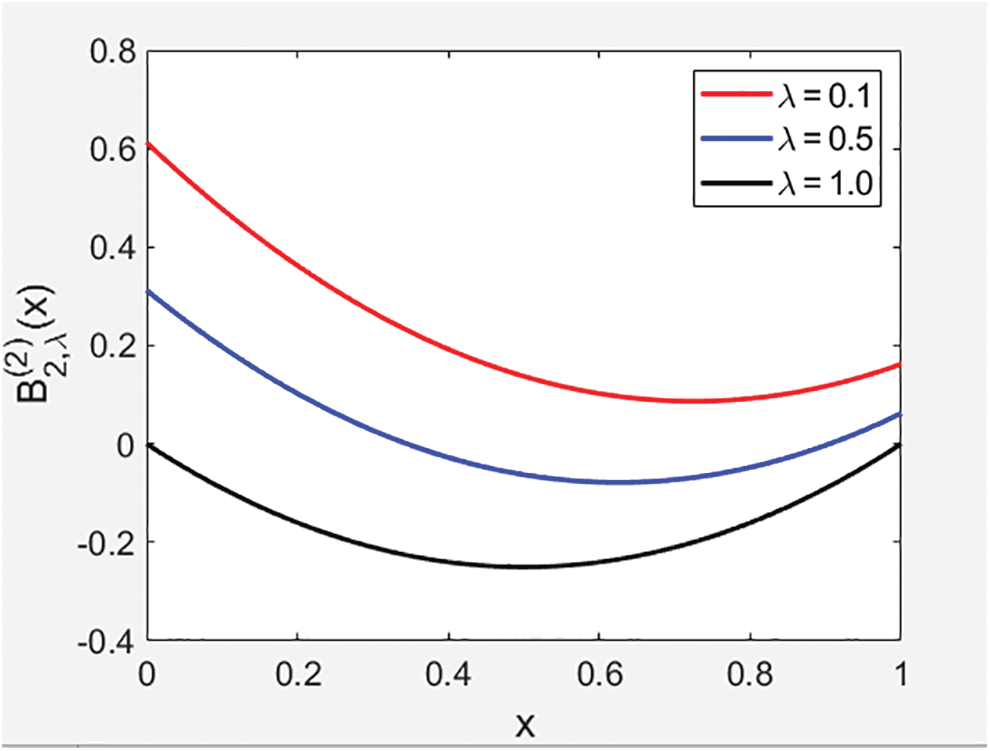
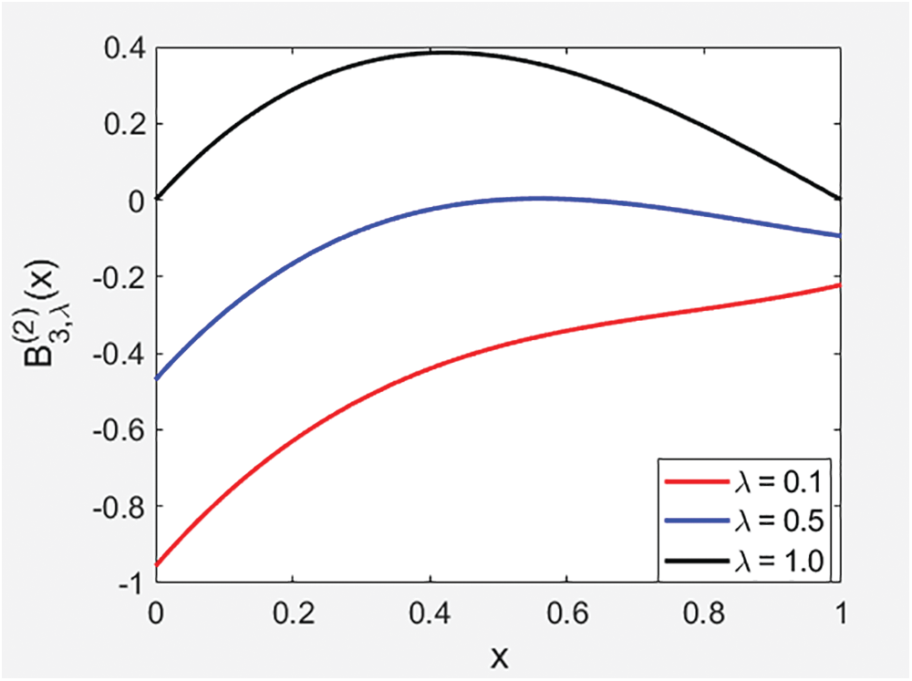
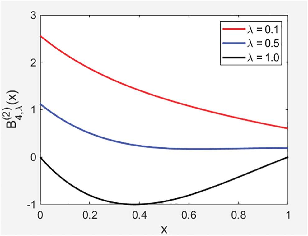
B2,λ(2)(x)=536(5-6λ+λ2)+32(-1+λ)x+x(x-λ),B3,λ(2)(x)=148(-53+74λ-31λ2+10λ3)+1536(5-6λ+λ2)x+94(-1+λ)x(x-λ)+x(x-λ)(x-2λ),B4,λ(2)(x)=11800(5477-9195λ+5045λ2-525λ3-802λ4)+112(-53+74λ-31λ2+10λ3)x+56(5-6λ+λ2)x(x-λ)+3(-1+λ)x(x-λ)(x-2λ)+x(x-λ)(x-2λ)(x-3λ).(28)

Now, using (28) and with the help of mathematica we plot B2,λ(2)(x), B3,λ(2)(x), and B4,λ(2)(x) in the following Figs. 1–3.

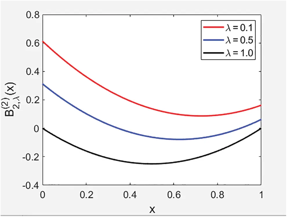
Figure 1: B2,λ(2)(x)

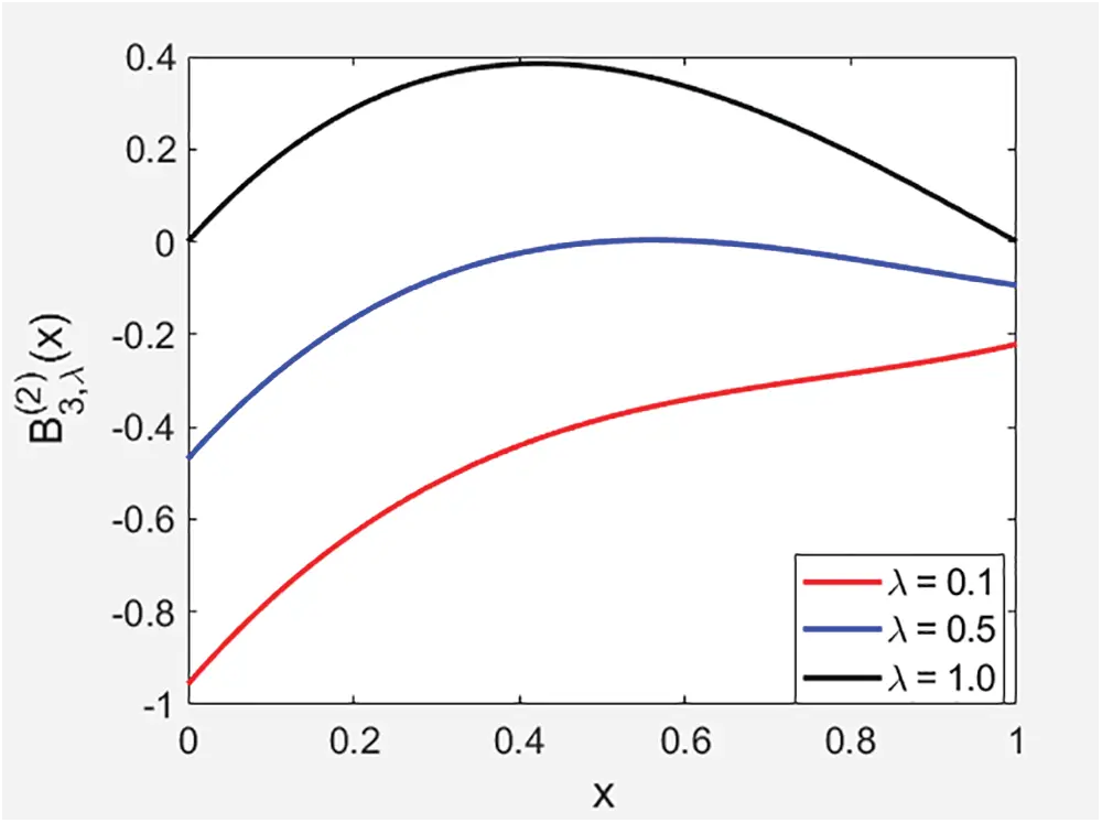
Figure 2: B3,λ(3)(x)

Figure 3: B4,λ(4)(x)

By (17) and (23), we get

(eλ(t)-1Eik,λ(logλ(1+t)))λBn,λ(k)(x)=(x)n,λ,(n≥0).(29)

Now, we observe

Eik,λ(logλ(1+t))eλ(t)-1=∑l=1∞(1)l,λlk-11l!(logλ(1+t))l1eλ(t)-1=∑l=1∞(1)l,λlk-1∑j=l∞S1,λ(j,l)tjj!1eλ(t)-1=∑j=1∞∑l=1j(1)l,λlk-1S1,λ(j,l)tjj!1eλ(t)-1=∑j=0∞∑l=1j+1(1)l,λS1,λ(j+1,l)lk-1(j+1)tjj!teλ(t)-1=∑j=0∞∑l=1j+1(1)l,λS1,λ(j+1,l)lk-1(j+1)tjj!∑m=0∞βm,λtmm!=∑n=0∞(∑j=0n∑l=1j+1(nj)(1)l,λS1,λ(j+1,l)lk-1(j+1)βn-j,λ)tnn!.(30)

From (29) and (30), we note that

Bn,λ(k)(x)=(Eik(logλ(1+t))eλ(t)-1)λ(x)n,λ=(∑m=0∞∑j=0m∑l=1j+1(mj)(1)l,λS1,λ(j+1,l)lk-1(j+1)βm-j,λtmm!)λ(x)n,λ=∑m=0n∑j=0m∑l=1j+1(mj)(nm)(1)l,λS1,λ(j+1,l)lk-1(j+1)βm-j,λ(x)n-m,λ.(31)

Therefore, by (31), we obtain the following theorem:

Theorem 2.2. For n≥0, we have

By (10) and (11), we get

Bn,λ(k)(y)=〈Eik,λ(logλ(1+t))eλ(t)-1eλy(t)|(x)n,λ〉=〈Eik,λ(logλ(1+t))t|(teλ(t)-1eλy(t))λ(x)n,λ〉λ=∑l=0n(nl)βl,λ(y)〈Eik,λ(logλ(1+t))t|(x)n-l,λ〉λ=∑l=0n(nl)βl,λ(y)(n-l+1)〈Eik(logλ(1+t))|(x)n-l+1,λ〉λ=∑l=0n(nl)βl,λ(y)(n-l+1)〈∑m=1∞(1)m,λmk-1m!(logλ(1+t))m|(x)n-l+1,λ〉λ=∑l=0n(nl)βl,λ(y)(n-l+1)〈∑j=1∞(∑m=1j(1)m,λmk-1S1,λ(j,m))tjj!|(x)n-l+1,λ〉λ=∑l=0n(nl)βl,λ(y)(n-l+1)∑m=1n-l+1(1)m,λmk-1S1,λ(n-l+1,m)=∑l=0n∑m=1n-l+1(nl)βl,λ(y)(n-l+1)(1)m,λmk-1S1,λ(n-l+1,m).(32)

Therefore, by (32), we obtain the following theorem:

Theorem 2.3. For n≥0, we have

The fully degenerate Bell polynomials are defined as

eλx(eλ(t)-1)=∑n=0∞Beln,λ(x)tnn!.(33)

Note that

∑n=0∞limλ→0Beln,λ(x)tnn!=ex(et-1)=∑n=0∞Beln(x)tnn!.(34)

By comparing the coefficients on both sides of (34), we have

where Beln(x) are the ordinary Bell polynomials.

From (33), we note that

Beln,λ(x)~(1,logλ(1+t))λ.(35)

References

1. Carlitz, L. (1979). Degenerate stirling, Bernoulli and Eulerian numbers. Utilitas Mathematica, 15, 51–88. [Google Scholar]
2. Carlitz, L. (1956). A degenerate Staudt–Clausen theorem. Archiv der Mathematik (Basel), 7(1), 28–33. DOI 10.1007/BF01900520. [Google Scholar] [CrossRef]
3. Chung, S. K., Jang, G. W., Kim, D. S., Kwon, J. (2019). Some identities of the type 2 degenerate Bernoulli and Euler numbers. Advanced Studies in Contemporary Mathematics (Kyungshang), 29(4), 613–632. [Google Scholar]
4. Kim, D. S., Kim, T. (2021). Degenerate Sheffer sequences and λ-Sheffer sequences. Journal of Mathematical Analysis and Applications, 493(1), 124521. DOI 10.1016/j.jmaa.2020.124521. [Google Scholar] [CrossRef]
5. Kim, D. S., Kim, T. (2020). A note on a new type of degenerate Bernoulli numbers. Russian Journal of Mathematical Physics, 27(2), 227–235. DOI 10.1134/S1061920820020090. [Google Scholar] [CrossRef]
6. Kim, H. K. (2020). Degenerate Lah–Bell polynomials arising from degenerate Sheffer sequences. Advances in Difference Equations, 2020(1), 1–16. [Google Scholar]
7. Kim, T., Kim, D. S. (2020). Degenerate polyexponential functions and degenerate Bell polynomialss. Journal of Mathematical Analysis and Applications, 487(2), 124017. DOI 10.1016/j.jmaa.2020.124017. [Google Scholar] [CrossRef]
8. Kim, T., Kim, D. S., Kwon, J., Lee, H. (2020). Degenerate polyexponential functions and type 2 degenerate poly-Bernoulli numbers and polynomials. Advances in Difference Equations, 2020(1), 1–12. DOI 10.1186/s13662-020-02636-7. [Google Scholar] [CrossRef]
9. Lee, D. S., Kim, H. K. (2020). On the new type of degenerate poly-Genocchi numbers and polynomials. Advances in Difference Equations, 2020(1), 1–15. DOI 10.1186/s13662-020-02886-5. [Google Scholar] [CrossRef]
10. Araci, S. (2014). Novel identities involving Genocchi numbers and polynomials arising from applications of umbral calculus. Applied Mathematics and Computation, 233(2), 599–607. DOI 10.1016/j.amc.2014.01.013. [Google Scholar] [CrossRef]
11. Dere, R., Simsek, Y. (2012). Applications of umbral algebra to some special polynomials. Advanced Studies in Contemporary Mathematics (Kyungshang), 22(3), 433–438. [Google Scholar]
12. Ma, Y., Kim, D. S., Lee, H., Kim, H., Kim, T. (2021). Reciprocity of poly-dedekind-type DC sums involving poly-Euler functions. Advances in Difference Equations, 2021(1), 1–18. [Google Scholar]
13. Boyadzhiev, K. N. (2007). Polyexponentials. https://arxiv.org/abs/0710.1332. [Google Scholar]
14. Kim, D. S., Kim, T. (2019). A note on polyexponential and unipoly functions. Russian Journal of Mathematical Physics, 26(1), 40–49. DOI 10.1134/S1061920819010047. [Google Scholar] [CrossRef]
15. Hardy, G. H. (1905). On the zeroes of certain classes of integral Taylor series. Part II. On the integral function formula and other similar functions. Proceedings of the London Mathematical Society, 2(2), 401–431. [Google Scholar]
16. Hardy, G. H. (1905). On the zeroes certain classes of integral Taylor series. Part I. On the integral function formula. Proceedings of the London Mathematical Society, 2(2), 332–339. [Google Scholar]
17. Andrews, L. C. (1985). Special functions for applied mathematics and engineering. New York: MacMillan. [Google Scholar]
18. Roman, S. (1984). The umbral calculus. Pure and applied mathematics, vol. 111. New York: Academic Press, Inc. [Google Scholar]
19. Comtet, L. (1974). Advanced combinatorics: The art of finite and infinite expansions. Dordrecht and Boston: Reidel (Translated from the French by J. W. Nienhuys). [Google Scholar]