Computer Modeling in Engineering & Sciences

DOI: 10.32604/cmes.2021.016761

ARTICLE

A Reliability Evaluation Method for Intermittent Jointed Rock Slope Based on Evolutionary Support Vector Machine

Shuai Zheng, An-Nan Jiang* and Kai-Shuai Feng

College of Transportation Engineering, Dalian Maritime University, Dalian, 116026, China
*Corresponding Author: An-Nan Jiang. Email: jiangannan@163.com
Received: 24 March 2021; Accepted: 07 July 2021

1  Introduction

Evaluation of slope stability should always be considered in geotechnical engineering such as tunnel portal sections, foundation pit slope releases and highway subgrade. Due to the influence of weathering, geological movement and other natural factors, the slope often contains intermittent joints. Variations in joint length, joint inclination angle and other parameters result in uncertainty of the slope stability [1–3]. Therefore, when evaluating slope stability, it is necessary to consider the intermittent state of the joints.

Researchers often try to obtain rock mass parameters through sampling tests to judge the stability of geotechnical engineering [4–6]. This method can evaluate rock mass properties, but it is unable to take into consideration the randomness problem in real-world engineering. The reliability method is an effective technique in describing the engineering uncertainty and in recent years has been gradually incorporated into the evaluation of stability of slope engineering. For example, Chen et al. [7] used the point estimation method to evaluate the reliability of the subgrade slope stability. Sasanian et al. [8] analyzed slope reliability by the geotechnical random field method. Huang et al. [9] analyzed slope stability under seismic conditions. Aladejare et al. [10] analyzed the relationship between rock properties and slope reliability. In these studies, the researchers were able to evaluate the status of slope reliability, but they all used the limit equilibrium method based on rigid assumptions. Because the mapping relationship between joint parameters and slope stability is very complicated in actual engineering, it is difficult to describe it with general analytical methods. Numerical simulation can achieve the restoration and analysis of complex projects, but the rate of calculation is so slow that it is difficult to meet the fast-mapping requirements in the reliability evaluation process. Therefore, it is necessary to establish a response surface model to express the relationship between the slope joint parameters and the slope safety factors to solve this problem.

Machine learning algorithms are continually being developed and applied to express complex mapping relations in geotechnical engineering, such as support vector machine (SVM) [11], artificial neural network (ANN) [12,13] and Gaussian process regression (GPR) [14,15]. These algorithms are also widely used in vibration control [16], blasting risk prediction [17] and the development of new materials [18]. Although their applicability in the field of geotechnical engineering has been widely verified, researchers have also found that the machine learning algorithms have a certain degree of parameter dependency. To solve this problem, biological optimization strategies have been formed to optimize the parameters of these models, such as particle swarm optimization (PSO) [19], differential evolution (DE) [20], bacterial foraging optimization algorithm (BFOA) [21], tabu search (TS) [22] and simulated annealing (SA) [23]. Some calculation methods combining machine learning algorithms and an optimization strategy have achieved good results in the evaluation of slope stability. For example, Fei et al. [24] used surrogate models via a new SVM to analyze slope stability, and Wang et al. [25] studied the landslide problem through Bayesian back analysis.

Most current slope reliability studies assume that the joints are continuous [26,27], and that the reliability evaluation method for intermittent jointed rock slope requires further discussion. Also requiring further study are the sensitivity of geometrical parameters of intermittent joints and the mapping relation between them and the slope safety factors. In addition, conventional intelligent algorithms still face the problem of parameter and sample dependence and cannot meet the requirements for evaluation of the reliability of intermittent jointed slope. This study aims to develop a hybrid intelligent algorithm to establish a response surface model to express the mapping function between joint parameters and the slope safety factor, and then to evaluate the slope reliability.

Compared with other machine learning models, least squares support vector machine (LSSVM) has faster calculation speed and a more concise theoretical model, which can be applied to data learning under the condition of small samples and is suited for reliability analysis of jointed slopes. To resolve the problem of kernel parameter dependence, which frequently occurs in LSSVM, this study uses the BFOA strategy with good global optimization ability. The joint finite element method is used to simulate the intermittent jointed slope model and to form the learning samples by parameter orthogonal design. Next, the BFOA-LSSVM is trained to express the mapping relationship between the slope joint parameters and the safety factor and is used to replace the finite element in order to speed up the calculation. A large number of parameter groups are established by Monte Carlo sampling, the slope safety factor of each group is obtained by BFOA-LSSVM, and the results were statistically analyzed to obtain the slope reliability.

2  Reliability Evaluation Method for Intermittent Jointed Rock Slope

Due to the randomness of joint parameters, the reliability evaluation of jointed rock slopes is very complicated, and the efficiency of numerical analysis is low. In this study, the BFOA-LSSVM was trained based on the data samples obtained from the joint finite element method, in order to perform the rapid evaluation of the intermittent joint slope reliability.

2.1 Reliability Evaluation

Fig. 1 shows the intermittent joints in actual engineering and defines the parameters that can describe the distribution characteristics of such joints. Of these, θ is the joint inclination angle, d is the joint spacing, L is the joint length and k=L/L1 is the persistence coefficient. The random distribution of these parameters leads to uncertainty of the slope. To solve this problem, the reliability method is adopted.

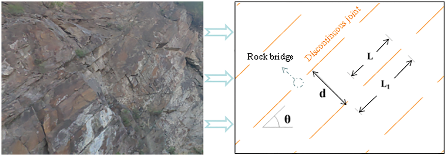
Figure 1: Intermittent joints distribution in the rock mass

Reliability is a probabilistic measure of a structure’s ability to perform a predetermined function at a specified time and under specified conditions [28]. For slope joint parameters group X, the failure probability of the slope is given by Eq. (1).

Pf=P(g(X)<0)=∫g(X)<0h(X)dX, (1)

where h(X) is the joint probability density function of four slope joint parameters, and g(X) is the limit state function, which can be calculated by Eq. (2) for the slope engineering.

g(X)=F(X)−1, (2)

where F(X) is the response surface function, which represents the mapping relationship between the intermittent joints parameters and the slope safety factor.

The relationship between joint parameters and the slope safety factors expressed by F(X) in Eq. (2) is a complex implicit relationship. It is difficult for this relationship to be described by general functions, which leads to the difficulty of calculating Eq. (1). To solve this problem, the LSSVM is used to express this mapping relationship.

2.2 Response Surface Function Established by LSSVM

Regression calculation of LSSVM is the process of fitting known data through a hyperplane [29]. For the training samples {xi,yi}i=1…N (where xi∈R4 are the slope joint parameters and yi∈R1 is the safety factor), the response surface function established by LSSVM regression can be expressed as Eq. (3).

F(x)=∑k=1iαkK(x,xk)+b, (3)

where kernel function K(x,xk) adopts radial basis function, K(x,xk)=exp⁡{−‖x−xk‖2/σ2}, σ2 is the square bandwidth, which represents the influence degree of a single sample, αk is a Lagrangian operator and b is the amount of paranoia, calculated by Eq. (4).

[0LTLΩ+γ−1I][bα]=[0y], (4)

where y=[y1,y2,…,yi], L is an array with I dimensions, L=[1,1,…,1], Ω=φ(xk)Tφ(xl)=K(xk,xl), α=[α1,α2,…,αi], k,l=1,2,…,N, I is the unit vector and γ is the regular parameter representing the interval fitting degree.

LSSVM offers the advantages of simple structure and fast calculation speed, but at the same time, it is also faced with the problem of parameter dependence, which is frequently found in intelligent algorithms. The BFOA strategy is used to find the optimal solution for the parameters of LSSVM in order to obtain a more accurate mapping model.

2.3 Evolutionary Response Surface Model

The BFOA [30] optimization strategy simulates the foraging behavior of human E. coli and searches for the optimal solution through iterative calculation. Compared with other biological heuristic algorithms, BFOA has a simple principle and mechanism structure, robustness and good global optimization ability, which means it can avoid falling into a locally optimal solution. It also has low dependence on the initial value of a single parameter. Therefore, BFOA is used to optimize the key parameters of LSSVM in order to improve the accuracy of the response surface model. There are eight steps to the implementation of BFOA.

(1) Set the BFOA initialization parameters, include the size of the bacterial community S, the dimension of the space in which the bacterial community was located P, the upper limit times of trend, replication, and migration Nc,Nre,Ned, the single trend step length of the trend operation C(i), the maximum number of single forward steps Ns and the migration probability Ped.

(2) Generate initial population randomly in the parameter optimization interval. Each bacterium represents a set of LSSVM parameters (γ,σ2). The two-dimensional vector of information contained in the Nth bacterium can be expressed as θn=[θ1n,θ2n].

(3) Divide the learning samples into training samples and testing samples. The current position of each bacterium is taken as the individual value, and then the LSSVM model is substituted for regression prediction to obtain the corresponding safety factor.

(4) Evaluate the adaptive value of the current population through Eq. (5).

Fve=[∑t=1S0(yt−y′t)2]/S0, (5)

where yt and y′t are the predicted and actual safety factors, respectively, S0 is the population number and Fve is the population fitness.

For the expected adaptive value Fvmin, if the current population meets Fvmin≤Fve, then enter Step (8). Otherwise, entry Step (5).

(5) Adjust the current population with a single step C(i) and repeat this process Nc times.

(6) Record the position with the minimum fitness value in Step (5), sort the population at that position according to individual fitness value, delete half of the individuals with the larger fitness value and copy the other half to keep the population quantity unchanged. Return to Step (4) until Step (6) is repeated Nre times and then enter Step (7).

(7) Delete the current population and return to Step (2). If Step (7) has been performed Ned times, then enter Step (8).

(8) The optimal parameter (γ,σ2) calculated in Step (7) is used as the parameter of LSSVM to establish the regression model between the joint parameters and the slope safety factor.

The above process obtains a complete BFOA-LSSVM model, but before using it to build the response surface function, it is necessary to prepare the corresponding learning samples through joint finite element calculation.

2.4 Joint Finite Element Calculation for Learning Samples

Numerical calculation models of fractures can be divided into discrete element discontinuous models [31] and finite element continuous models [32]. The former is mainly used to describe large-scale deformation of joints such as opening and sliding, and the latter mainly describes the properties of joints as contact surfaces [33,34]. The joints of the slope in this study are in contact, which can be described by the contact unit of the continuous medium.

The RS2 finite element software package developed by Canadian company Rocscience was selected as the calculation platform. The jointed rock mass is regarded as a binary structure composed of rock blocks and joints, in which the joint part is simulated by the Goodman unit.

The Goodman unit is a thickness-free unit, which is often used to simulate the soft structural plane in rock mass. It proposes four nodes without thickness and eight degrees of freedom units (as shown in Fig. 2). The lines 1–2 and 3–4 are two contact surfaces connected by tiny springs in the middle. The normal RS2 stiffness coefficient is kn, and the tangential stiffness coefficient is ks. Assuming the model is linear elastic contact, its constitutive relation is expressed as Eq. (6).

{σnτs}=[kn00ks]{ωnωs} (6)

where σn is the normal stress on the joint surface, τs is the tangential stress of the joint surface, ωn is the normal displacement of the joint surface and ωs is the tangential displacement of the joint surface.

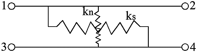
Figure 2: Goodman joint unit

The mechanical properties of friction strength and deformation at the contact surface of the element under external force are described by strength and deformation parameters. Therefore, the Goodman unit can simulate the tangential force and deformation characteristics of joints. RS2 finite element software corrected the Goodman element’s defect of embedding both sides of the contact surface into each other under pressure, allowing the joint parts to dislocate each other, resulting in tangential and normal displacement and plastic yield of the joint part.

The orthogonal design of joint parameters is carried out through engineering investigation to ensure that the design samples can cover the range of the actual parameters. The slope safety factor is obtained by the strength reduction method based on joint finite element calculation, with the two critical conditions being displacement mutation and shear zone transfixion, and the Mohr-Coulomb failure criterion used for both rock blocks and joints. The strength reduction formula is shown in Eq. (7).

{c′=c/FsrJc′=Jc/Fsr{φ′=arctan⁡(tan⁡φ/Fsr)Jφ′=arctan⁡(tan⁡Jφ/Fsr) (7)

where c′ and φ′ are the reduced cohesion and the friction angle of rock blocks, respectively, J′c and J′φ are the reduced cohesion and the friction angle of joints, respectively, and Fsr is the reduction coefficient.

Compared with the limit equilibrium method, the strength reduction method is more suited for the intermittent jointed slope, because it can reflect the stress-strain relation of the slope rock mass, and it does not need to manually set the range of slip surface.

2.5 Slope Reliability Evaluation Process Based on Evolutionary Response Surface

According to the orthogonal design samples of the parameters, the learning samples are formed by the finite element method calculation. This sample is used to train BFOA-LSSVM to establish the response surface between the intermittent joint parameters and the slope safety factor. For an engineering structure that needs to be evaluated, each intermittent joint parameter is evaluated at different locations on the site and its distribution characteristics are counted. The Monte Carlo sampling of these parameters is performed by computer programming, forming a large number of parameter groups, using the trained BFOA-LSSVM model to obtain the slope safety factor corresponding to each group, and then using these results to obtain the slope reliability.

Next, the reliability evaluation model for the intermittent joint slope is established. The logical relationship and calculation process are shown in Fig. 3.

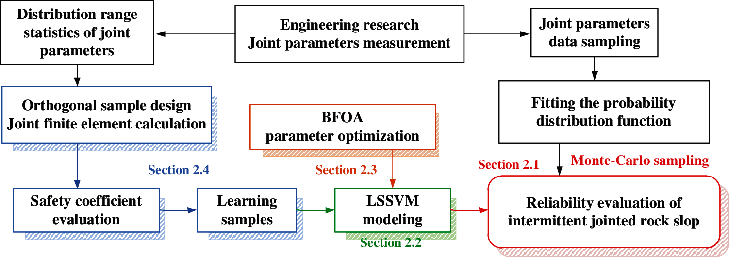
Figure 3: Flow chart of reliability evaluation for rock slope with intermittent joints

3  Engineering Application

3.1 Engineering Cases

The highway from Dandong to Altay in Jilin Province of China has many potential risks in the area of the slope along the Yalu River. In order to ensure the safety of highway operations, a comprehensive slope safety assessment is planned in this area. Using section K235 + 800 ~ K235 + 950 as an example, the slopes of these areas are about 0.5 m away from the left edge of the road. The main body of the slope is composed of strongly weathered basalt, with blocky structure and relatively developed joints and fissures. The engineering position and the actual state of the slope body are shown in Fig. 4.

Figure 4: Project location and its actual status

Combined with the geological survey and field investigation results, the distribution range of joint parameters in this section is joint inclination angle θ∈[0∘,80∘], joint spacing d∈[2 m,4m], joint length L∈[4m,6m] and persistence coefficient k ∈ [0.4, 0.8].

In order to obtain the learning samples required for LSSVM training, an orthogonal design of geometric parameters of intermittent joints is carried out based on the survey results, forming a total of 35 orthogonal test pieces, as shown in Appendix A. Orthogonal design can fully consider the combination of different factors and solve the corresponding slope safety factor from the orthogonal sample through finite element calculation, so as to establish a relatively complete learning sample.

Because the interval in this case study was relatively short and the distribution range of joint parameters was relatively concentrated, the orthogonal design sample was determined to be 35 groups. In the actual application process, when the target interval is long or the joint parameter distribution is relatively scattered, the number of orthogonal samples should be correspondingly expanded to meet the training needs of the machine learning model.

3.2 Safety Factor Evaluation

An engineering numerical calculation model was built according to the field survey drawings. The bottom and both sides of the model are fully constrained, while the top part is the free boundary. The entire slope is divided by free triangle elements, and the dimensions of each structure are shown in Fig. 5.

Figure 5: Numerical calculation model

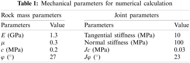
In order to record the slope deformation, four displacement measure points were uniformly arranged on the slope surface. In addition to the joint geometric parameters, the rock mass and joint mechanical parameters were sampled on-site and obtained through laboratory tests, as shown in Tab. 1. The intermittent joint model was used for calculation, and the joint geometric parameters were assigned based on the orthogonal design data.

Next, we assigned the physical parameters in Tab. 1 to the geometric model shown in Fig. 5, and calculated the slope safety factors under different joint geometric parameters, as shown in Appendix A. We used Group 13 as an example to introduce the process of determining the safety factors. Fig. 6 shows the displacement monitoring results and a slope shear strain cloud diagram of this sample under different reduction factors. It can be seen that when the reduction coefficient exceeds 1.35, the displacement changes abruptly (Fig. 6a), and the shear surface tends to penetrate (Fig. 6b). When the reduction coefficient increases to 1.42 and 1.44, the shear surface develops rapidly and the displacement rises rapidly (Figs. 6c and 6d). Based on this, the safety factor of this sample group is determined to be 1.35. The slope safety factor of each orthogonal group in Appendix A was calculated one by one to form the learning samples, and the results are listed in the last column of Appendix A. This set of data was used to train the LSSVM model, as discussed in Section 2.2, and to determine the optimal solution search of model parameters through BFOA, establish evolutionary algorithms to solve the problem of parameter dependence and improve the accuracy of the model.

Figure 6: Slope shear strain under strength reduction: (a) Deformation curve under strength reduction (b) Strength reduction coefficient 1.35, (c) Strength reduction coefficient 1.42 (d) Strength reduction coefficient 1.44

3.3 Statistics and Validation of Engineering Joint Parameters

We counted the joint development states in the target area through the investigation of the slope exposed surface. Using the slope of K216 + 750 ~ K216 + 900 as an example, the joint angle in this area is close to 45°, the spacing is about 3 m and the length of a single joint is about 5 m. The results of each parameter are shown in Tab. 2, and the specific distribution is shown in Fig. 7.

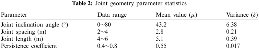
Figure 7: Statistical graph of joint parameter data: (a) Joint angle statistical results (b) Joint spacing statistical results (c) Joint length statistical results and (d) Persistence coefficient statistical results

3.4 Analysis of Slope Reliability Calculation Results

We trained LSSVM using the learning samples obtained in Section 3.2, where the first 30 groups are used as training samples, and the remaining five groups are used as test samples. The parameter optimization results of LSSVM through BFOA are γ=5.210, σ2=27.167. We performed a slope reliability evaluation based on the intermittent joint parameters, as discussed in Section 3.3. The Monte Carlo sampling was conducted according to the results of parameters in Tab. 2, and the sampling number was set to 105. The average safety factor of the target slope is 1.48 and the variance is 0.03. Fig. 8 shows the specific distribution of the calculation results.

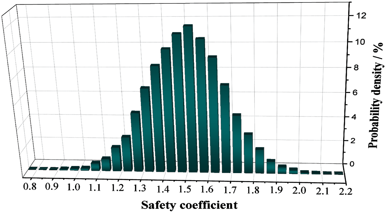
Figure 8: Safety factor distribution histogram

Some safety factors in Fig. 8 are less than 1, indicating that there the project still carries a certain risk. However, the average safety factor is moderate and the variance is small, which illustrates that the overall stability of the slope engineering is good. Although there is no risk of a large-scale landslide failure, more attention should be paid to local dangers such as falling blocks. Experts have investigated and evaluated this area and determined that its safety factor is 1.57, which is consistent with the most probable safety factor in the evaluation results of this project, shows that the research method is feasible.

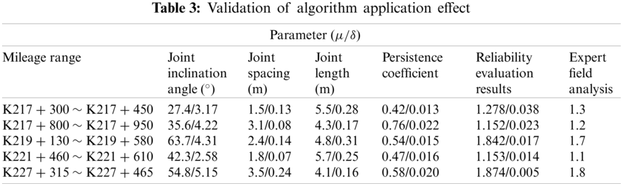
To further illustrate the accuracy of the BFOA-LSSVM response surface model and reliability evaluation method established by this research, several typical sections were selected for a group of experts to conduct an on-site evaluation. The results of this evaluation are shown in Tab. 3. The average value of the reliability calculation results in the table is basically consistent with that of the evaluation results of the expert group, which shows that this method is suited for the reliability evaluation of discontinuous joint slopes. Combined with Fig. 8, it can be seen that the reliability method can provide more complete evaluation information, as well as a comprehensive reference for slope disaster prevention.

3.5 Joint Parameter Sensitivity Analysis by Reliability Evaluation

The above research process established a method to calculate the slope reliability through the joint parameters, through which the sensitivity of the joint parameters can be analyzed based on the changes in reliability.

We adjusted the mean value of the parameters in turn, keeping the other parameters unchanged in order to carry out the Monte Carlo process. The slope reliability index under the condition of different mean values of different parameters is shown in Fig. 9, where the severe changes in the reliability index due to the different mean values indicate the greater degree of influence of this parameter on slope reliability.

Figure 9: Joint geometric parameter influence curve: (a) Effect of joint angle on calculation results (b) Effect of joint spacing on calculation results (c) Effect of joint length on calculation results and (d) Effect of joint bridge ratio on calculation results

The reliability index in the figure is defined as:

β=μ/(1−δ) (8)

where μ and δ are the mean and variance value of the safety factor, respectively.

It can be seen in Fig. 9 that the incidence of the four joint parameters on the slope reliability from large to small is joint length → joint inclination angle → joint spacing → persistence coefficient. Therefore, attention should be mainly paid to the development of joint length in the construction process, and anchor injection reinforcement should be carried out according to the joint inclination angle state.

4  Discussion

4.1 Influence of LSSVM Parameters on Regression Results

To illustrate this problem, using the actual measured data of the project based on this research as an example (the project situation described in Chapter 3), we adjusted the regular parameter γ and square bandwidth σ2 of LSSVM and performed trial calculations on the samples, as shown in Appendix A. The relative error statistics of the regression results of the test samples under different parameter combinations are shown in Fig. 10. Because it is an irregular surface, the minimum error area (purple area) of the optimal parameter is distributed in a curved strip.

Fig. 10 shows that the key parameters of LSSVM have a significant impact on the accuracy of the regression results. However, the optimal solution of the key parameters does not converge to a specific value, but needs to search continuously in an irregular interval, which demonstrates the necessity of parameter optimization for LSSVM during the establishment of the response surface model.

Figure 10: Sensitivity analysis of LSSVM parameters

4.2 Advantage Analysis of BFOA-LSSVM Response Surface

Machine learning models such as Gaussian process regression (GPR), artificial neural network (ANN), and LSSVM, which are commonly used in geotechnical engineering, were used to perform regression comparisons on the test samples. The relative error statistics of the prediction results calculated by different algorithms are shown in Fig. 11. The initial parameters of each algorithm were obtained through trial calculations based on the test sample through the “cross multiplication”. The specific parameter settings are marked in Fig. 11. In the ANN model, Nf is the number of hidden layer nodes of the algorithm, Ep is the number of iterations and Lr is the learning rate. In the GPR model, σN is the noise standard deviation of the algorithm, and σf is the local correlation coefficient.

Figure 11: Regression effects of different algorithms

It can be seen that the LSSVM has a significant advantage over the other two algorithms in prediction accuracy, which is mainly attributed to the small sample learning ability. The regression accuracy of LSSVM optimized by BFOA is obviously improved. Depending on the robustness and global optimization function of the BFOA, the coupling algorithm can search for the optimal parameters of LSSVM, thereby realizing the accurate expression of the mapping relationship between the intermittent joint parameters and the slope safety factor. The comparison shows that the algorithm proposed in this research is effective.

4.3 Validity Analysis of Sampling Number in Monte-Carlo Calculation

To study the influence of the number of Monte Carlo sampling on the calculation results, the slope of K216 + 750 ~ K216 + 900 in Section 3.3 was again used as an example, and different sampling comparisons were carried out. The variation coefficient VC shown in Eq. (9) was used to analyze the discreteness of the results, where μ and δ are the mean and variance value of the safety factor calculated for 10 consecutive times under the same conditions, respectively.

VC=(δ/μ)×100 (9)

The μ and δ data and variation coefficient curve under different sampling numbers are shown in Fig. 12. It can be observed that the average value of the results in each group is almost the same, but the variation coefficient is large when the sampling number is small, which represents the volatility of the calculation results. This means the accuracy of the single sampling results is poor at this time. With the increase in sampling number, the calculated results tend to be more stable. Accordingly, it is recommended that the sampling times should not be less than 104 during the application of the method established in this study.

Figure 12: Discrete analysis of reliability evaluation results under different sampling number

5  Conclusion

This study established a reliability evaluation method for intermittent jointed rock slope, evaluated the safety factor by strength reduction based on joint finite element calculation, and then developed the BFOA-LSSVM hybrid algorithm/machine learning model to establish a response surface model for expressing the mapping relationship between the slope joint parameters and the safety factors. The successful application of this method on the slope of the Yalu River in China reflects its feasibility. This paper offers the following four main findings.

(1) The reliability evaluation method fully takes into account the uncertainty of the slope joint parameters. It can offer a more comprehensive evaluation of the slope safety results, thereby providing a complete data reference for engineering construction.

(2) The BFOA-LSSVM hybrid response surface model, which can accurately express the mapping relationship between joint parameters and slope safety factors, achieved rapid slope evaluation. Comparative calculations show that this model performs better than GPR and ANN in evaluation of intermittent jointed rock slope.

(3) Joint length and joint angle play key roles in the intermittent jointed rock slope stability. Attention should be paid to the development of joint length in the construction process, and anchor injection reinforcement should be carried out according to the joint inclination angle state.

(4) During the application of the method established in this study, it is recommended that the Monte Carlo sampling number be no less than to ensure the accuracy of results.

The joint survey in this study is a statistical analysis of the slope surface, which leads to conservative evaluation results. In future research, it is recommended that geological radar and other technical means be used to detect the joint development inside the slope to obtain more accurate evaluation results. Further studies should also focus on the randomness of the shear strength parameters of the slope rock mass.

Acknowledgement: The authors thank LetPub (https://www.letpub.com) for its linguistic assistance during the preparation of this manuscript.

Funding Statement: The authors sincerely appreciate the support from the National Natural Science Foundation of China [Grant Nos. 51678101, 52078093], Liaoning Revitalization Talents Program [Grant No. XLYC1905015], and the Doctoral innovation Program of Dalian Maritime University [Grant No. BSCXXM016].

Conflicts of Interest: The authors declare that they have no conflicts of interest to report regarding the present study.

References

 1.  Ning, Y. J., Zhao, Z. Y., Sun, J. P., Yuan, W. F. (2012). Using the discontinuous deformation analysis to model wave propagations in jointed rock masses. Computer Modeling in Engineering & Sciences, 89(3), 221–262. DOI 10.3970/cmes.2012.089.221. [Google Scholar] [CrossRef]

 2.  Yan, Y., Dai, Q., Jin, L., Wang, X. (2019). Geometric morphology and soil properties of shallow karst fissures in an area of karst rocky desertification in SW China. Catena, 174(6), 48–58. DOI 10.1016/j.catena.2018.10.042. [Google Scholar] [CrossRef]

 3.  Deng, Z. P., Li, D. Q., Qi, X. H., Cao, Z. J., Phoon, K. K. (2017). Reliability evaluation of slope considering geological uncertainty and inherent variability of soil parameters. Computers and Geotechnics, 92(3), 121–131. DOI 10.1016/j.compgeo.2017.07.020. [Google Scholar] [CrossRef]

 4.  Fan, J., Liu, W., Jiang, D., Chen, J., Tiedeu, W. N. et al. (2020). Time interval effect in triaxial discontinuous cyclic compression tests and simulations for the residual stress in rock salt. Rock Mechanics and Rock Engineering, 53(9), 4061–4076. DOI 10.1007/s00603-020-02150-y. [Google Scholar] [CrossRef]

 5.  Bérest, B. B., Karimi, J. M., Sambeek, L. V. (2007). Transient behavior of salt caverns-interpretation of mechanical integrity tests. International Journal of Rock Mechanics & Mining Sciences, 44(5), 767–786. DOI 10.1016/j.ijrmms.2006.11.007. [Google Scholar] [CrossRef]

 6.  Fan, J. Y., Jiang, D. Y., Liu, W. (2019). Discontinuous fatigue of salt rock with low-stress intervals. International Journal of Rock Mechanics and Mining Sciences, 115, 77–86. DOI 10.1016/j.ijrmms.2019.01.013. [Google Scholar] [CrossRef]

 7.  Chen, Z., Du, J., Yan, J., Sun, P., Li, K. et al. (2019). Point estimation method: Validation, efficiency improvement, and application to embankment slope stability reliability analysis. Engineering Geology, 105232. DOI 10.1016/j.enggeo.2019.105232. [Google Scholar] [CrossRef]

 8.  Sasanian, S., Soroush, A., Chenari, R. J. (2019). Slope reliability analysis using the geotechnical random field method. Geotechnical Engineering, 172(6), 1–41. DOI 10.1680/jgeen.19.00016. [Google Scholar] [CrossRef]

 9.  Huang, H. W., Wen, S. C., Zhang, J., Chen, F. Y., Martin, J. R. et al. (2018). Reliability analysis of slope stability under seismic condition during a given exposure time. Landslides, 15(11), 2303–2313. DOI 10.1007/s10346-018-1050-9. [Google Scholar] [CrossRef]

10. Aladejare, A. E., Wang, Y. (2017). Influence of rock property correlation on reliability analysis of rock slope stability: From property characterization to reliability analysis. Geoscience Frontiers, 9(6), 1639–1648. DOI 10.1016/j.gsf.2017.10.003. [Google Scholar] [CrossRef]

11. Wen, T., Tang, H. M., Wang, Y. K. (2017). Landslide displacement prediction using the GA-LSSVM model and time series analysis: A case study of Three Gorges Reservoir. Natural Hazards and Earth System Sciences, 17(12), 2181–2198. DOI 10.5194/nhess-17-2181-2017. [Google Scholar] [CrossRef]

12. Karaci, A., Yaprak, H., Ozkaraca, O., Demir, I., Simsek, O. (2019). Estimating the properties of ground-waste-brick mortars using DNN and ANN. Computer Modeling in Engineering & Sciences, 118(1), 207–228. DOI 10.31614/cmes.2019.04216. [Google Scholar] [CrossRef]

13. Zhang, Y. Z. (2019). Application of improved BP neural network based on e-commerce supply chain network data in the forecast of aquatic product export volume. Cognitive Systems Research, 57(21), 228–235. DOI 10.1016/j.cogsys.2018.10.025. [Google Scholar] [CrossRef]

14. Hu, B., Su, G. S., Jiang, J. Q. (2019). Uncertain prediction for slope displacement time-series using Gaussian process machine Learning. IEEE Access, 7, 27535–27546. DOI 10.1109/ACCESS.2019.2894807. [Google Scholar] [CrossRef]

15. Gao, W., Karbasi, M., Hasanipanah, M., Zhang, X., Guo, J. (2018). Developing GPR model for forecasting the rock fragmentation in surface mines. Engineering with Computers, 34(3), 1–7. DOI 10.1007/s00366-017-0544-8. [Google Scholar] [CrossRef]

16. Hasanipanah, M., Monjezi, M., Shahnazar, A., Armaghani, D. J., Farazmand, A. (2015). Feasibility of indirect determination of blast induced ground vibration based on support vector machine. Measurement, 75(3), 289–297. DOI 10.1016/j.measurement.2015.07.019. [Google Scholar] [CrossRef]

17. Hasanipanah, M., Shahnazar, A., Arab, H., Golzar, S. B., Amiri, M. (2016). Developing a new hybrid-AI model to predict blast-induced backbreak. Engineering with Computers, 33(3), 349–359. DOI 10.1007/s00366-016-0477-7. [Google Scholar] [CrossRef]

18. Chen, X., Shi, X., Zhang, S., Chen, H., Zhou, J. et al. (2020). Fiber-reinforced cemented paste backfill: The effect of fiber on strength properties and estimation of strength using nonlinear models. Materials, 13(3), 718. DOI 10.3390/ma13030718. [Google Scholar] [CrossRef]

19. Yang, Z., Sun, W. (2013). A set-based method for structural eigenvalue analysis using Kriging model and PSO algorithm. Computer Modeling in Engineering & Sciences, 92(2), 193–212. DOI 10.3970/cmes.2013.092.193. [Google Scholar] [CrossRef]

20. Lobato, F. S. (2010). Self-adaptive differential evolution based on the concept of population diversity applied to simultaneous estimation of anisotropic scattering phase function, albedo and optical thickness. Computer Modeling in Engineering & Sciences, 69(1), 1–17. DOI 10.3970/cmes.2010.069.001. [Google Scholar] [CrossRef]

21. Zeng, Z. G., Guan, L. H., Zhu, W. Q. (2019). Face recognition based on SVM optimized by the improved bacterial foraging optimization algorithm. International Journal of Pattern Recognition and Artificial Intelligence, 33(7), 1–9. DOI 10.1142/S021800141956007X. [Google Scholar] [CrossRef]

22. Li, Y. C., Lian, S. D. (2018). Improved fruit fly optimization algorithm incorporating tabu search for optimizing the selection of elements in trusses. KSCE Journal of Civil Engineering, 23(6), 4940–4954. DOI 10.1007/s12205-017-2000-0. [Google Scholar] [CrossRef]

23. Lamberti, L., Pappalettere, C. (2007). Weight optimization of skeletal structures with multi-point simulated annealing. Computer Modeling in Engineering & Sciences, 18(3), 183–221. DOI 10.3970/cmes.2007.018.183. [Google Scholar] [CrossRef]

24. Fei, K., Qing, X., Jun, J. L. (2016). Slope reliability analysis using surrogate models via new support vector machines with swarm intelligence-sciencedirect. Applied Mathematical Modelling, 40(11–12), 6105–6120. DOI 10.1016/j.apm.2016.01.050. [Google Scholar] [CrossRef]

25. Wang, Y., Huang, J., Tang, H., Zeng, C. (2020). Bayesian back analysis of landslides considering slip surface uncertainty. Landslides, 17(9), 2125–2136. DOI 10.1007/s10346-020-01432-4. [Google Scholar] [CrossRef]

26. Zhang, J., Huang, H. W., Juang, C. H., Li, D. Q. (2013). Extension of Hassan and Wolff method for system reliability analysis of soil slopes. Engineering Geology, 160(6), 81–88. DOI 10.1016/j.enggeo.2013.03.029. [Google Scholar] [CrossRef]

27. Zeng, P., Jimenez, R., Jurado-Piña, R. (2015). System reliability analysis of layered soil slopes using fully specified slip surfaces and genetic algorithms. Engineering Geology, 193, 106–117. DOI 10.1016/j.enggeo.2015.04.026. [Google Scholar] [CrossRef]

28. Scholkopf, B., Sung, K. K., Burges, C. J., Girosi, F., Niyogi, P. et al. (1997). Comparing support vector machines with Gaussian kernels to radial basis function classifiers. IEEE Transactions on Signal Processing, 45(11), 2758–2765. DOI 10.1109/78.650102. [Google Scholar] [CrossRef]

29. Xu, X. H., Qu, G. G., Fang, L. G. (2010). Reliability analysis of rock slope based on uncertainty of joint geometric parameters. Journal of Central South University of Science and Technology, 41(3), 1139–1145. DOI 10.1016/S1876-3804(11)60004-9. [Google Scholar] [CrossRef]

30. Passino, K. M. (2002). Biomimicry of bacterial foraging for distributed optimization and control. IEEE Control System Magazine, 22(3), 52–67. DOI 10.1109/MCS.2002.1004010. [Google Scholar] [CrossRef]

31. Xu, G., He, C., Yang, Q., Wang, B. (2019). Progressive failure process of secondary lining of a tunnel under creep effect of surrounding rock. Tunnelling and Underground Space Technology, 90(48), 76–98. DOI 10.1016/j.tust.2019.04.024. [Google Scholar] [CrossRef]

32. Azarfar, B., Ahmadvand, S., Sattarvand, J. (2019). Stability analysis of rock structure in large slopes and open-pit mine: Numerical and experimental fault modeling. Rock Mechanics and Rock Engineering, 52(12), 4889–4905. DOI 10.1007/s00603-019-01915-4. [Google Scholar] [CrossRef]

33. Fazio, N., Perrotti, M., Andriani, G., Mancini, F., Rossi, P. et al. (2019). A new methodological approach to assess the stability of discontinuous rocky cliffs using in-situ surveys supported by UAV-based techniques and 3-D finite element model: A case study. Engineering Geology, 260(2), 105205. DOI 10.1016/j.enggeo.2019.105205. [Google Scholar] [CrossRef]

34. Pain, A., Kanungo, D. P., Sarkar, S. (2014). Rock slope stability assessment using finite element based modelling-examples from the Indian Himalayas. Geomechanics & Geoengineering, 9(3), 215–230. DOI 10.1080/17486025.2014.883465. [Google Scholar] [CrossRef]

Appendix A. Learning Samples Generated by Orthogonal Design

This work is licensed under a Creative Commons Attribution 4.0 International License, which permits unrestricted use, distribution, and reproduction in any medium, provided the original work is properly cited.