| Computer Modeling in Engineering & Sciences |
DOI: 10.32604/cmes.2021.016758
ARTICLE
Weighted Parameterized Correlation Coefficients of Indeterminacy Fuzzy Multisets and Their Multicriteria Group Decision Making Method with Different Decision Risks
1Beijing Urban Construction Group Co., Ltd., Beijing, 100088, China
2School of Civil and Environmental Engineering, Ningbo University, Ningbo, 315211, China
*Corresponding Author: Jun Ye. Email: yejun1@nbu.edu.cn
Received: 24 March 2021; Accepted: 08 May 2021
Abstract: Real-life data introduce noise, uncertainty, and imprecision to statistical projects; it is advantageous to consider strategies to overcome these information expressions and processing problems. Neutrosophic (indeterminate) numbers can flexibly and conveniently represent the hybrid information of the partial determinacy and partial indeterminacy in an indeterminate setting, while a fuzzy multiset is a vital mathematical tool in the expression and processing of multi-valued fuzzy information with different and/or same fuzzy values. If neutrosophic numbers are introduced into fuzzy sequences in a fuzzy multiset, the introduced neutrosophic number sequences can be constructed as the neutrosophic number multiset or indeterminate fuzzy multiset. Motivated based on the idea, this study first proposes an indeterminate fuzzy multiset, where each element in a universe set can be repeated more than once with the different and/or identical indeterminate membership values. Then, we propose the parameterized correlation coefficients of indeterminate fuzzy multisets based on the de-neutrosophication of transforming indeterminate fuzzy multisets into the parameterized fuzzy multisets by a parameter (the parameterized de-neutrosophication method). Since indeterminate decision-making issues need to be handled by an indeterminate decision-making method, a group decision-making method using the weighted parameterized correlation coefficients of indeterminate fuzzy multisets is developed along with decision makers’ different decision risks (small, moderate, and large risks) so as to handle multicriteria group decision-making problems in indeterminate fuzzy multiset setting. Finally, the developed group decision-making approach is used in an example on a selection problem of slope design schemes for an open-pit mine to demonstrate its usability and flexibility in the indeterminate group decision-making problem with indeterminate fuzzy multisets.
Keywords: Indeterminate fuzzy multiset; parameterized correlation coefficient; multicriteria group decision making; neutrosophic number; slope design scheme
Fuzzy sets (FSs) and fuzzy multisets (FMs) are vital mathematical tools in the expression and processing of fuzzy information since there are uncertainty and vagueness in many real-life problems. In the fuzzy theory, the FS presented by Zadeh [1] is depicted by a degree of membership, which usually contains almost one occurrence of each element in FS. Since then, fuzzy sets have wildly applied in various areas [2–9]. As an extension of FS, Yager [10] and Miyamoto [11] proposed the concept of fuzzy bag/FM, where each element in a universe set can be repeated more than once with the different and/or identical membership values. Then, FMs have been used for various applications in many areas [12–15]. Recently, El-Azab et al. [16] proposed a correlation coefficient of FMs as the extension of a correlation coefficient of FSs [17] and gave its application in the setting of FMs. Further, Das [18] put forward weighted fuzzy soft multiset (WFSM) and introduced an adjustable approach to the WFSMs-based decision-making method in uncertain environment. Furthermore, an interval-valued fuzzy multiset (IvFM) [19] was presented as the extension of FMs, where each element in a universe set can be repeated more than once with the different and/or identical membership values. In the hesitant fuzzy environment, then, a hesitant fuzzy set (HFS) and an interval-valued hesitant fuzzy set (IvHFS) [20] were represented by a group of different fuzzy values, but they cannot reflect the same fuzzy values in a group of hesitant fuzzy values. Under indeterminate and inconsistent environments, the neutrosophic multisets with the same or different neutrosophic components were proposed based on truth, falsity and indeterminacy membership functions and used for the applications in physical processes [21,22].
Due to the vagueness and indeterminacy of human cognition/judgments in complicated real problems, the human judgment may contain the hybrid information of the partial determinacy and partial indeterminacy. However, FMs and fuzzy soft multisets cannot represent the indeterminate fuzzy sequences, while a neutrosophic/indeterminate number (NN/IN) [23–25] is composed of its determinate term d and its indeterminate term uI with indeterminacy I ∈ [inf I, sup I] and denoted as z = d + uI for d, u ∈
Since FMs, HFSs, IvFMs, and IvHFSs cannot express indeterminate fuzzy sequences by the indeterminate membership values in group decision making (GDM) problems with indeterminate information, various measure algorithms of FMs, HFSs, IvFMs, and IvHFSs cannot also deal with such GDM problems with the indeterminate fuzzy sequences and indeterminate decision risks of decision makers because indeterminate decision-making problems need to be solved by an indeterminate decision making method. If NNs/INs are introduced into fuzzy sequences in FMs and IvFMs, we can produce indeterminate/NN fuzzy sequences from the different and/or identical indeterminate membership values with some indeterminate ranges and construct an indeterminate fuzzy multiset (IFM) so as to present the parameterized correlation coefficients (PCCs) of IFMs by a parameterized de-neutrosophication method of IFM for handling indeterminate GDM problems with decision makers’ different decision risks. Motivated by these new ideas, this study proposes IFM, where each element in a universe set can be repeated more than once with the different and/or identical indeterminate membership values, and then introduces two PCCs of IFMs based on the de-neutrosophication of transforming IFMs into the parameterized fuzzy multisets (PFMs) by a parameter λ ∈ [0, 1] (i.e., the parameterized de-neutrosophication method) and their GDM approach with decision makers’ different decision risks (small, moderate and large risks for λ = 0, 0.5, 1) to solve indeterminate GDM problems in IFM setting.
However, main contributions of this study are summarized as follows:
1. The proposed IFM contains various families of FMs, HFSs, IvFMs, and IvHFSs depending on the indeterminate ranges and values of I and provides an expression form of the different and/or identical indeterminate membership values that HFS and IvHFS cannot express.
2. The proposed two PCCs of IFMs based on the parameterized de-neutrosophication method can provide effective mathematical models for solving indeterminate decision-making problems because the correlation coefficient of FMs cannot deal with indeterminate decision-making issues.
3. The developed GDM method based on the two PCCs can solve indeterminate GDM problems, such as the selecting problem of slope design schemes (SDSs) for an open pit mine with decision makers’ different decision risks in the actual indeterminate application and show its highlighting advantages of the practicability and flexibility in IFM setting.
This paper is composed of the following parts. Section 2 introduces preliminaries of FMs. Section 3 proposes IFM and two PCCs of IFMs based on the de-neutrosophication of transforming IFMs into PFMs by a parameter λ ∈ [0, 1]. Section 4 develops a GDM method using PCCs of IFMs along with decision makers’ different decision risks (small, moderate and large risks for λ = 0, 0.5, 1) in IFM setting. In Section 5, the developed GDM method is used in a GDM example on a selection problem of SDSs for an open pit mine with decision makers’ different decision risks to demonstrate the usability and flexibility of the developed GDM method in IFM setting. Conclusions and further research are contained in Section 6.
In FM/fuzzy bag presented by Yager [10], each element yj in a universe set Y = {y1, y2, …, ys} can be repeated more than once with the different and/or identical membership values. Then, a FM B is denoted as
Let two FMs be B1 = {b11, b12, …, b1s} and B2 = {b21, b22, …, b2s}, where
where
Based on the properties of the correlation coefficient between FMs [16], the weighted correlation coefficient Nw(B1, B2) should imply the following properties:
(i) Nw(B1, B2) = Nw(B2, B1);
(ii) Nw(B1, B2) = 1 iff B1 = B2;
(iii) Nw(B1, B2) ∈ [0, 1].
Based on the hybrid concept of FMs [16] and NNs [23–25], this section presents the concept of IFM, the relations of IFMs, and the de-neutrosophication approach of IFM with a parameter λ ∈ [0, 1], and then proposes two PCCs of IFMs.
Definition 3.1. Set Y = {y1, y2, …, ys} as a universe set. An IFM M over Y is presented by the following mathematical symbol:
where
For instance,
Especially when qj = 1 (j = 1, 2, …, s) in Z, the IFM Z is reduced to the indeterminate FS. Then, FM/IvFM is a special case of IFM with a specified value I = inf I = sup I or a specified interval value I = [inf I, sup I] since IFM contains a family of IFMs/FMs corresponding to a group of specified indeterminate ranges/values of I.
Then, each component
Definition 3.2. Set two NNFSs as
(1) z1j(I) ⊇ z2j(I) ⇔
(2) z1j(I) = z2j(I) ⇔ z1j(I) ⊇ z2j(I) and z2j(I) ⊇ z1j(I);
(3)
(4)
(5)
For the de-neutrosophication of IFM, a parameter λ ∈ [0, 1] can be introduced to transform IFM into PFM with λ ∈ [0, 1] based on a parameterized de-neutrosophication method.
Definition 3.3. Let Z = {z1(I), z2(I), …, zs(I)} be an IFM, where
Obviously, each zj(λ) (j = 1, 2, …, s) changes as the value of λ ∈ [0, 1] changes under a specifical range of I ∈ [inf I, sup I]. Thus, PFM with λ indicates a family of FMs corresponding to a group of values of λ ∈ [0, 1], while FM is only a special case of PFM for a specifical value of λ.
Based on the correlation coefficient of FMs [16], we propose two PCCs between two IFMs based on PFMs with λ ∈ [0, 1].
Definition 3.4. Let two IFMs be Z1 = {z11(I), z12(I), …, z1s(I)} and Z2 = {z21(I), z22(I), …, z2s(I)}, where
By applying Eq. (4), the parameterized correlations between Z1 and Z1 and between Z2 and Z2 are given as follows:
which are also named the parameterized informational energy of IFMs Z1 and Z2.
Consequently, the two PCCs of IFMs Z1 and Z2 based on PFMs with λ ∈ [0, 1] are proposed by
Regarding the properties of the correlation coefficient of FMs [16], the PCCs
(i)
(ii)
(iii)
Proof: Obviously, the properties (i) and (ii) are straightforward. Hence, we only verify the property (iii).
According to the Cauchy-Schwarz inequality
Hence, it is obvious that there also exists the following inequality for λ ∈ [0, 1]:
Thus,
Therefore, this proof is completed.
When we consider the importance of each NNFS zkj (k = 1, 2; j = 1, 2, …, s) in Z1 and Z2, we specify the weight ηj ∈ [0, 1] of zkj with
Similarly, the weighted PCCs
(i)
(ii)
(iii)
By the similar proof way regarding the properties of the two PCCs, we can easily verify the above properties (i)–(iii).
4 GDM Approach Based on the Weighted PCCs in IFM Setting
Corresponding to the weighted PCCs of IFMs, we develop a GDM approach with decision makers’ different decision risks in IFM setting.
Regarding multicriteria GDM problems in indeterminate setting, suppose experts/designers preliminarily specify a set of p potential alternatives G = {g1, g2, …, gp}, which is evaluated by a set of s criteria C = {c1, c2, …, cs}. The weight vector of C is given as η = (η1, η2, …, ηs) to consider the importance of different criteria. Then, a group of q decision makers is invited to give the satisfactory assessments of an alternative gi (i = 1, 2, …, p) over criteria cj (j = 1, 2, …, s), which are expressed by the NNFSs
In multicriteria GDM problems with IFM information, we can develop a GDM approach using the weighted PCCs of IFMs with decision makers’ different decision risks (the small, moderate and large risks for λ = 0, 0.5, 1), which is depicted by the decision steps below:
Step 1: The ideal solution/alternative can be specified by:
Step 2: By using Eq. (9) or Eq. (10) with decision makers’ different decision risks (the small, moderate, and large risks for λ = 0, 0.5, 1), the weighted PCC between Zi (i = 1, 2, …, p) and Z* is yielded by the following formula:
Or
Step 3: The alternatives are ranked based on the values of the weighted PCC depending on the decision makers’ different decision risks, then the best one is chosen.
Step 4: End.
Regarding an open pit mine, the design problem of the slopes is one of the major challenges at mine planning and operation [32]. It requires specialized knowledge of the geology, which is often complex, vague, and indeterminate/variable in the structural and material properties of orebodies. Regarding this indeterminate issue, we provide a GDM example on the selection problem of SDSs for an open pit mine to show the usability and flexibility of the developed GDM method with different decision risks of decision makers in IFM setting.
A mining company wants to select the best SDS/alternative regarding an open pit mine. Assume a set of four potential SDSs (alternatives) G = {g1, g2, g3, g4} for the open pit mine is specified preliminarily by experts/designers. Then, the four alternatives must be satisfactorily assessed over the three criteria/indices: economy (cost and construction period) (c1), technology (reliability, effectiveness, construction difficulty, maintenance difficulty, and safety) (c2), and environment (c3). Considering the importance of the three criteria, the experts/designers give the weight vector of the three criteria by
In the GDM problem, three experts/decision makers are specified and then their satisfactory assessments of the four alternatives gi (i = 1, 2, 3, 4) over the three criteria cj (j = 1, 2, 3) are given by the NNFSs
Thus, the developed GDM approach is utilized for the multicriteria GDM problem with IFMs for I ∈ [0, 1] and described by the following calculations:
First, the ideal solution/alternative is specified by
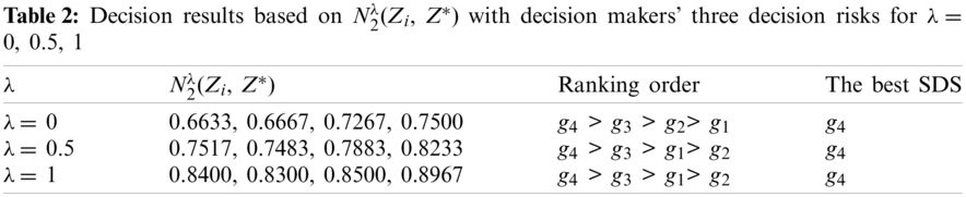
Then, the weighted PCC values between IFMs Zi (i = 1, 2, 3, 4) and Z* are calculated by Eq. (11) or Eq. (12) along with the decision makers’ small risk for λ = 0, moderate risk for λ = 0.5, large risk for λ = 1 in the indeterminate range of I ∈ [inf I, sup I] = [0, 1], which are shown in Tabs. 1 and 2.
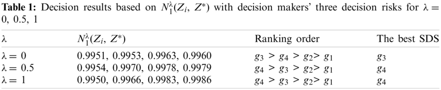
Regarding the decision results based on N1λ(Zi, Z*) in Tab. 1, the ranking orders of alternatives indicate their difference between the decision makers’ small risk (λ = 0) and the decision makers’ moderate and large risks (λ = 0.5, 1), then the best SDS is g3 for λ = 0 or g4 for λ = 0.5, 1. However, the ranking orders based on N1λ(Zi, Z*) imply the sensitivity to the decision makers’ different decision risks.
Regarding the decision results based on N2λ(Zi, Z*) in Tab. 2, the ranking orders of alternatives indicate a little difference between the decision makers’ small risk (λ = 0) and the decision makers’ moderate and large risks (λ = 0.5, 1), then the best SDS is g4 for all decision risks. However, the ranking orders based on N2λ(Zi, Z*) imply a little sensitivity to the decision makers’ different decision risks.
Furthermore, the ranking orders and the best SDSs based on N1λ(Zi, Z*) and N2λ(Zi, Z*) also show their difference, which implies the sensitivity between two weighted PCCs. It is obvious that either the different weighted PCCs or the decision makers’ different decision risks may impact on the ranking orders of alternatives. Then, the final decision result depends on the weighted PCC and decision risk selected by decision makers in the specified indeterminate range of I ∈ [inf I, sup I], which demonstrates the usability and flexibility of the proposed GDM method in IFM setting.
To compare the proposed PCCs of IFMs with the existing correlation coefficient of FMs [16] in fuzzy decision-making problems, we first indicate the characteristic comparison between IFMs and the classical FMs from the perspective of their information expression, which is shown in Tab. 3.
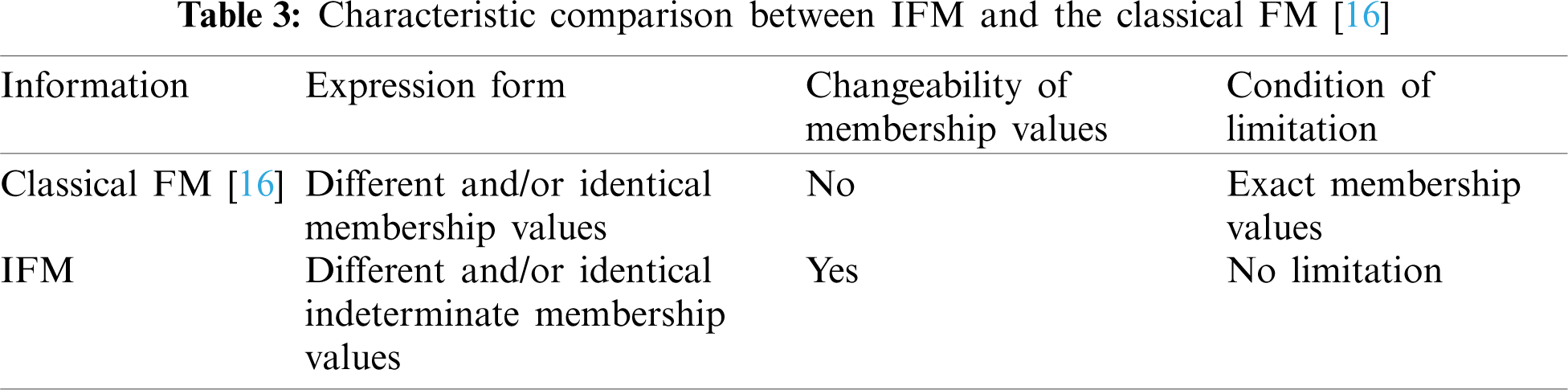
Regarding the comparative results of Tab. 3, IFM is often broader and more versatile than the classical FM in the information expression and usability, which show the outstanding advantage of IFM in indeterminate setting.
Especially, the existing correlation coefficient of FMs [16] is only a special case of the proposed PCC of IFMs when λ only takes a specified value. Obviously, the decision-making approach based on the correlation coefficient of FMs [16] is also a special case of the developed GDM method in IFM setting. In their decision making process, the existing decision making approach cannot contain decision makers’ different decision risks sine FMs cannot contain NNs (changeable/indeterminate interval values), then it lacks the decision making flexibility in the indeterminate scenarios, while the developed GDM method can contain decision makers’ different decision risks for satisfying some suitable indeterminacy by using the decision information of PFMs in the setting of IFMs and also indicate the flexible decision making advantage with various indeterminate decision risks in the indeterminate problem. Therefore, the proposed GDM method can overcome difficult/tricky decision-making problems of the existing FM decision making method in indeterminate issues because indeterminate decision-making issues need to be solved by utilizing an indeterminate decision-making method generally. However, this study proposes the GDM method by using the weighted PCCs of IFMs to solve such an indeterminate multicriteria GDM problem with decision makers’ different decision risks (the small, moderate, and large risks for λ = 0, 0.5, 1) for the first time in IFM setting.
However, the information expression, correlation coefficient and GDM methods of IFMs proposed in this study are superior to existing methods [16].
Regarding the indeterminate multi-values of fuzzy arguments in indeterminate GDM setting, the proposed IFM in this paper presented a more flexible and useful information expression form as it addresses the indeterminacy of multi-fuzzy values corresponding to various indeterminate ranges/values of the indeterminacy I ∈ [inf I, sup I]. Then, the presented PCCs of IFMs based on the de-neutrosophication of transforming IFMs into PFMs by a parameter λ ∈ [0, 1] provided effective mathematical models for the flexible GDM method in indeterminate environment. The developed multicriteria GDM method using the weighted PCCs of IFMs along with decision makers’ different decision risks (the small, moderate, and large risks for λ = 0, 0.5, 1) provided an effect and reasonable decision way for handling indeterminate multicriteria GDM problems in IFM setting. A GDM example of selecting the best SDS for an open pit mine was given in the environment of IFMs to demonstrate the suitability and flexibility of the developed GDM method. Then, the decision results indicated the influence of decision makers’ different decision risks on the ranking order of alternatives and the best one. Therefore, the developed multicriteria GDM method can reflect its outstanding advantages of decision versatility and flexibility when dealing with indeterminate GDM problems under various decision risks.
In future research, this original work will be extended to GDM problems in construction design schemes, project management, and slope stability evaluation, and analyses under IFM environment.
Funding Statement: The authors received no specific funding for this study.
Conflicts of Interest: The authors declare that they have no conflicts of interest to report regarding the present study.
1. Zadeh, L. A. (1965). Fuzzy sets. Information and Control, 8(3), 338–353. DOI 10.1016/S0019-9958(65)90241-X. [Google Scholar] [CrossRef]
2. Pal, S. K., King, R. A. (1983). On edge detection of X-ray images using fuzzy sets. IEEE Transaction on Pattern Analysis and Machine Intelligence, 5, 69–77. DOI 10.1109/TPAMI.1983.4767347. [Google Scholar] [CrossRef]
3. Nguyen, V. U. (1985). Tender evaluation by fuzzy sets. Journal of Construction Engineering and Management, 111, 231–243. DOI 10.1061/(ASCE)0733-9364(1985)111:3(231). [Google Scholar] [CrossRef]
4. Yager, R. R. (1996). Database discovery using fuzzy sets. International Journal of Intelligent Systems, 11, 691–712. DOI 10.1002/(SICI)1098-111X(199609)11:9<691::AID-INT7>3.0.CO;2-F. [Google Scholar] [CrossRef]
5. Gurcanli, G. E., Mungen, U. (2009). An occupational safety risk analysis method at construction sites using fuzzy sets. International Journal of Industrial Ergonomics, 39, 371–387. DOI 10.1016/j.ergon.2008.10.006. [Google Scholar] [CrossRef]
6. Ansari, M., Hosseini, R. S., Sharifi, M. (2016). Evaluating and rating the performance of Qazvin municipalities, using the balanced scorecard (BSC) model, with fuzzy multi-criteria decision-making (FMCDM) approach. International Journal of Human-Computer Studies, 3(2), 185–197. [Google Scholar]
7. Rahimi, M., Najafi, A. (2016). Analysis of customer’s expectations and satisfaction in Zanjan municipality using fuzzy multi-criteria decision making (FMCDM) approach. Journal of Optimization in Industrial Engineering, 10(21), 47–57. DOI 10.22094/joie.2016.260. [Google Scholar] [CrossRef]
8. Pandey, M. M., Shukla, D., Graham, A. (2019). Evaluating the human performance factors of air traffic control in Thailand using fuzzy multi criteria decision making method. Journal of Air Transport Management, 81(6), 101708. DOI 10.1016/j.jairtraman.2019.101708. [Google Scholar] [CrossRef]
9. Bostancı, B., Erdem, N. (2020). Investigating the satisfaction of citizens in municipality services using fuzzy modeling. Socio-Economic Planning Sciences, 69(4), 100754. DOI 10.1016/j.seps.2019.100754. [Google Scholar] [CrossRef]
10. Yager, R. R. (1986). On the theory of bags. International Journal of General Systems, 13(1), 23–37. DOI 10.1080/03081078608934952. [Google Scholar] [CrossRef]
11. Miyamoto, S. (2001). Fuzzy multisets and fuzzy clustering of documents. 10th IEEE International Conference on Fuzzy Systems, pp. 1539–1542. Melbourne, Australia. [Google Scholar]
12. Banatre, J. P., Le Metayer, D. (1993). Programming by multiset transformation. Communications of the ACM, 36(1), 98–111. DOI 10.1145/151233.151242. [Google Scholar] [CrossRef]
13. Li, B. (1999). Fuzzy bags and application. Fuzzy Sets and Systems, 34, 67–71. DOI 10.1016/0165-0114(90)90127-R. [Google Scholar] [CrossRef]
14. Goldberg, D. E. (2002). The design of innovation: Lessons from and for competent genetic algorithms. Dordrecht, Netherlands: Kluwer Academic Publishers. [Google Scholar]
15. Miyamoto, S. (2009). Generalized bags, bag relations, and applications to data analysis and decision making. Modeling Decisions for Artificial Intelligence, 5861, 37–54. DOI 10.1007/978-3-642-04820-3. [Google Scholar] [CrossRef]
16. El-Azab, M. S., Shokry, M., Abo Khadra, R. A. (2017). Correlation measure for fuzzy multisets. Journal of the Egyptian Mathematical Society, 25(3), 263–267. DOI 10.1016/j.joems.2017.02.007. [Google Scholar] [CrossRef]
17. Chiang, D. A., Lin, N. P. (1999). Correlation of fuzzy sets. Fuzzy Sets and Systems, 102(2), 221–226. DOI 10.1016/S0165-0114(97)00127-9. [Google Scholar] [CrossRef]
18. Das, A. K. (2018). Weighted fuzzy soft multiset and decision-making. International Journal of Machine Learning & Cybernetics, 9(5), 787–794. DOI 10.1007/s13042-016-0607-y. [Google Scholar] [CrossRef]
19. Pramanik, T., Samanta, S., Pal, M. (2016). Interval-valued fuzzy planar graphs. International Journal of Machine Learning and Cybernetics, 7(4), 653–664. DOI 10.1007/s13042-014-0284-7. [Google Scholar] [CrossRef]
20. Farhadinia, B. (2013). Information measures for hesitant fuzzy sets and interval-valued hesitant fuzzy sets. Information Sciences, 240, 129–144. DOI 10.1016/j.ins.2013.03.034. [Google Scholar] [CrossRef]
21. Smarandache, F. (2017). Neutrosphic multiset applied in physical processes. Actualization of the Internet of Things, A FIAP Industrial Physics Conference, pp. 120–121. Monterey, USA. [Google Scholar]
22. Smarandache, F. (2017). Neutrosophic perspectives: Triplets, duplets, multisets, hybrid operators, modal logic, hedge algebras, and applications. Brussels, Belgium: Pons Publishing House. [Google Scholar]
23. Smarandache, F. (1998). Neutrosophy: Neutrosophic probability, set, and logic. USA: American Research Press. [Google Scholar]
24. Smarandache, F. (2013). Introduction to neutrosophic measure, neutrosophic integral, and neutrosophic probability. Columbus: Sitech & Education Publishing. [Google Scholar]
25. Smarandache, F. (2014). Introduction to neutrosophic statistics. Columbus, USA: Sitech & Education Publishing. [Google Scholar]
26. Chen, J. Q., Ye, J., Du, S. G. (2017). Scale effect and anisotropy analyzed for neutrosophic numbers of rock joint roughness coefficient based on neutrosophic statistics. Symmetry, 9(10), 208. DOI 10.3390/sym9100208. [Google Scholar] [CrossRef]
27. Li, C. Q., Ye, J., Cui, W. H., Du, S. Q. (2019). Slope stability assessment method using the arctangent and tangent similarity measure of neutrosophic numbers. Neutrosophic Sets and Systems, 27, 98–103. DOI 10.5281/zenodo.3275419. [Google Scholar] [CrossRef]
28. Ye, J. (2017). Bidirectional projection method for multiple attribute group decision making with neutrosophic numbers. Neural Computing and Applications, 28(5), 1021–1029. DOI 10.1007/s00521-015-2123-5. [Google Scholar] [CrossRef]
29. Ye, J. (2016). Fault diagnoses of steam turbine using the exponential similarity measure of neutrosophic numbers. Journal of Intelligent & Fuzzy Systems, 30(4), 1927–1934. DOI 10.3233/IFS-151903. [Google Scholar] [CrossRef]
30. Ye, J. (2018). Neutrosophic number linear programming method and its application under neutrosophic number environments. Soft Computing, 22(14), 4639–4646. DOI 10.1007/s00500-017-2646-z. [Google Scholar] [CrossRef]
31. Ye, J., Cui, W. H., Lu, Z. K. (2018). Neutrosophic number nonlinear programming problems and their general solution methods under neutrosophic number environments. Axioms, 7(1), 13. DOI 10.3390/axioms7010013. [Google Scholar] [CrossRef]
32. Read, J., Stacey, P. (2009). Guidelines for open pit slope design. USA: Taylor & Francis Group, CRC Press. [Google Scholar]
 | This work is licensed under a Creative Commons Attribution 4.0 International License, which permits unrestricted use, distribution, and reproduction in any medium, provided the original work is properly cited. |