Moving Least Squares Interpolation Based A-Posteriori Error Technique in Finite Element Elastic Analysis

Mohd Ahmed; Devender Singh; Saeed Qadhi; Nguyen Thanh

doi:10.32604/cmes.2021.014672

1Civil Engineering Department, College of Engineering, King Khalid University, Abha, 61421, Saudi Arabia
2Ministry of Information, Soochna Bhavan, CGO Complex, Delhi, 110003, India
3Urban Transport & Coastal Engineering Department, University of Transport and Communications, Hanoi, 100000, Vietnam
*Corresponding Author: Mohd Ahmed. Email: mall@kku.edu.sa
Received: 19 October 2020; Accepted: 11 June 2021

Abstract: The performance of a-posteriori error methodology based on moving least squares (MLS) interpolation is explored in this paper by varying the finite element error recovery parameters, namely recovery points and field variable derivatives recovery. The MLS interpolation based recovery technique uses the weighted least squares method on top of the finite element method's field variable derivatives solution to build a continuous field variable derivatives approximation. The boundary of the node support (mesh free patch of influenced nodes within a determined distance) is taken as circular, i.e., circular support domain constructed using radial weights is considered. The field variable derivatives (stress and strains) are recovered at two kinds of points in the support domain, i.e., Gauss points (super-convergent stress locations) and nodal points. The errors are computed as the difference between the stress from the finite element results and projected stress from the post-processed energy norm at both elemental and global levels. The benchmark numerical tests using quadrilateral and triangular meshes measure the finite element errors in strain and stress fields. The numerical examples showed the support domain-based recovery technique's capabilities for effective and efficient error estimation in the finite element analysis of elastic problems. The MLS interpolation based recovery technique performs better for stress extraction at Gauss points with the quadrilateral discretization of the problem domain. It is also shown that the behavior of the MLS interpolation based a-posteriori error technique in stress extraction is comparable to classical Zienkiewicz-Zhu (ZZ) a-posteriori error technique.

Keywords: Recovery points; field variable derivatives; effectivity; error recovery; support domain; error convergence

Errors are formed in the finite element technique by the very process of splitting the problem area into subdomains. Discretization errors, due to subdividing the problem into sub-regions, are reflected themselves as discontinuities in stress or stress components between elements and as a distortion of the real boundary stresses. The errors are also generated when the displacement interpolation polynomial does not accurately represent the behavior of the continuum. The current research trends in the field of finite element technique include the development of alternative approaches of error estimation to increase the effectivity of finite element codes for solving industrial problems [1]. Zienkiewicz [2] has listed some important achievement in finite element method and presented an outline of some problems need further attention. Chen et al. [3] present the review made to meshless method in the last two decades which is developed to overcome the drawbacks of the finite element techniques. A meshless method, Element Free Galerkin (EFG) Method, requires only nodal data, i.e., no element mesh and connectivity, to implement the MLS technique for the construction of the approximation and associates each node to a domain of influence or weights. The method requires background mesh for performing numerical integrations to construct the system matrices and the essential boundary conditions are implemented using modified variational forms such as the Lagrange multiplier methods the penalty method or Nitsche’s method [4,5]. A review on the state-of-the-art of wide applicability of finite element methods is given by Cen et al. [6].

Several methods have been proposed to recover the field variables or their derivatives and to enhance the accuracy of finite element solution. Among the existing error estimation techniques, the recovery type [7] error estimation is most popular. The essence of the technique is to use the difference between the values of more accurate recovered field variables or their derivatives and those given by the finite element solution as a measure of the elemental error. Zienkiewicz et al. [8] developed a local projection technique, called as super-convergent patch recovery technique, to estimate derivatives based on the least square fit of the local polynomial to the to the super convergent value of the derivatives. Niu et al. [9] suggested an extraction method for stress recovery and displacement from a finite element solution, with focus on the boundary stress extraction. The process is super-convergent in that the convergence of the quantities recovered is equivalent to the energy of the strain. Ubertini [10] has developed the recovery by patch equilibrium and recovery by patch compatibility to get improved stresses to the explicitly measured stresses. Rodenas et al. [11] have put forwarded the improvement of the super-convergent patch recovery (SPR) technique, called SPR-C technique (Constrained SPR) and found that the technique considerably enhances the accuracy of the recovered stress field and the elemental effectivity of the Zienkiewicz-Zhu error estimator. The post-processed improved finite element linear elasticity solution by applying the residual method with set of Neumann data for nonconforming elements is due to Kim et al. [12]. Mohite et al. [13] have used energy predictions over the element patches including ZZ type patch recovery to recover the exact solution of the displacement field and strains. Rodenas et al. [14] proposes error recovery based on moving least squares (MLS) technique to acquire smoothed stress field in which the continuity of the recovered field is given by the shape functions of the underlying mesh. They obtained a continuous recovered stress field that enforces the equilibrium constraints along the boundary and satisfies the internal equilibrium equation. Parret et al. [15] propose a method for getting improved recovery of stress field using domain decomposition method in heterogeneous structure. They have proposed the post-processing of stress field in a non-overlapping local domain or sub-structure that depend on the mesh connectivity. The procedure is different from the post-processing of stress field using mesh free nodal sub-domain MLS technique, the approach used in the present study. The MLS technique has advantage as the technique is simple to implement in domain discontinuities and continuity of the stress field is provided through the weight function, associated to nodes of the sub-domains. The mesh free MLS approach will not require special attention for application to heterogeneous structures.

Sharma et al. [16] proposed a technique for the recovery of stress for low-order 3D finite elements. They achieved the post-processed stress field by satisfying equilibrium in an average sense and projecting the directly computed stress field onto the conveniently chosen space. Breitkopf et al. [17] has discussed the different aspect of MLS based interpolation for application to three-dimensional solids. They emphasized that additional constraints, to get a unique solution for the considered node distributions, are required for extending the technique to higher dimensions. A coupled finite element-element-free Galerkin (EFG) method for three-dimensional mechanics problems is presented by Sukumar et al. [18]. The EFG method construct the trial functions for the variational principle using moving least square (MLS) approximations over the spheres or parallelepiped domains of influence. Cai et al. [19] proposed a combined error estimator, consisting of the explicit residual and the enhanced Zienkiewicz-Zhu (ZZ) error estimator, for the conforming finite element approach, and demonstrated that the developed estimator is accurate for all meshes. Dong et al. [20] proposed an error estimator based on element energy projection technique for finite element analysis in adaptive environment.

Ullah et al. [21] suggested an error estimation of the hybrid finite element method (FEM) and the Mesh-Fee Galerkin method based on local maximum entropy shape function for linear and nonlinear problems having material and geometric nonlinearities. The Zienkiewicz et al. super-convergent patch recovery for stresses and strains is used in the FE region of the problem domain, while the Chung et al. [22] error estimator is used in the mesh free method region. Kumar et al. [23] have developed several field transfer techniques, that can be used to reorganize data for complete re-meshing of the computational domain or for mesh regularization, resulting from an ALE (Arbitrary Lagrangian or Eulerian) formulation with super-convergence property on surface and volume. Ahmed et al. [24] proposed Galerkin-based mesh free recovery techniques for finite-element elastic analysis of mechanics problems. The investigation of error estimation using element free recovery approach is carried out by Ahmed et al. [25]. They have suggested optimal values of order of polynomial expansion in basis function and dilation parameter to form support domain to obtain the better-quality of error estimation.

The present study is a contribution to further investigate the mesh free MLS interpolation based a-posteriori error technique under different discretization scheme, recovery points, and recovered derivative of field variables. The mesh free methods are developed due to the limitation of finite element method (FEM) for situations in which distortion of elements occur such as for large domain changes and domain discontinuities. The continuous field variable derivative for meshless Galerkin method is obtained through local interpolation of the nodal field variable/ field variable derivative values using MLS procedure, which involve the inversion of a moment matrix for every point under consideration. The MLS interpolation based recovery technique uses the least squares method on top of the finite element method's field variable derivatives solution to build a continuous field variable derivatives approximation. The continuity of the field variable derivative in MLS procedure is provided by the weighting function considered [26]. The boundary of the node support is taken as circular, i.e., circular support domain constructed using radial weights in MLS method. The field variable derivatives (stress and strains) are recovered at two kinds of points in support domain, i.e., Gauss points (super-convergent stress locations) and nodal points. The field variable derivatives (stress and strains) are recovered at two kinds of recovery points, i.e., at Gauss points (at super-convergent stress locations) and nodal points. The errors in the finite element solution at local and global level are measured in energy norm. Numerical experiments are performed on elastic two-dimensional plates to show that a-posteriori error techniques based on MLS interpolation are accurate and reliable. The plate domain is discretization using linear triangular and quadrilateral elements. Four discretization schemes namely, triangular, quadrilateral, structured and unstructured schemes have been selected for the study. The performance of the MLS interpolation based error recovery method is compared with mesh dependent patch based ZZ a-posteriori error technique [27] in term of rate of convergence, effectivity, and adaptive refined meshes.

Considering the 2D-linear elastic problems with stress field (σ) and unknown displacements field (u), satisfying over a domain Ω that is bounded by Γ = Γt ∪ Γu and are governed by the following differential equation

where f is the body force vector, LT is the derivative operator, t¯ and u¯ are prescribed tractions and displacements on Γt and Γu, respectively and n is the unit outward normal on the boundary Γ = Γt ∪ Γu,

By finite element discretization, the displacements (u) of any point within an element are calculated based on the following equation:

where N is the matrix of the interpolation functions, also known as shape functions and d is the nodal displacement vector. The strains can be related to the nodal displacements by the following formula:

The error in computed state variable derivatives, i.e., stresses (eε,eε∗) or strains (eω,eω∗) is defined as the difference between the exact (close form solution, σ or ε) or recovered values (σ* or ε*) and respective computed values, σh (or εh), i.e.,

The errors can be measured in appropriate norms. The integral measure of the error in energy norm (E) may be defined as follows:

An estimator is asymptotically exact for a problem if the problem global and local (element) effectivity index (θ), i.e., ratio of estimated error and actual error, converges to one when the mesh size approaches to zero.

where ‖eex‖ and ‖e‖ denote the actual error and the estimated error estimate in energy norm.

The solution is acceptable if η ≤ ηallow where ηallow is the allowable accuracy. If η > ηallow, refinement is needed.

The success of the finite element error recovery depends largely on the accuracy of the post-processed solution. Different a-posteriori error techniques can be used to improve the quality of the recovered derivatives such as simple averaging, local or global projection and those exploring the super convergence phenomenon. The procedure given in literature [24] for classical mesh dependent patch based recovery technique, i.e., ZZ recovery, is followed in the present study. The MLS based a-posteriori error method employed for the recovery of stress or strain is described below.

The MLS approach provides a continuous approximation for the field function over the entire solution domain with reasonably accuracy, because of approach completeness, robustness, and continuity [28]. Recovery technique based on MLS interpolation derived the approx. functions by a set of nodes distributed over a patch or support domain (zone up to a determined distance with influenced nodes) (Fig. 1), without depending on the meshing scheme, in a weighted least square sense. “In MLS technique, three components are used to express the function u(x) with the approximation uh(x), a weight function w(x) associated to each node, a basis functions P(x), usually consisting of a polynomial, and a set of coeﬃcients a(x), which are functions of the coordinates. Let the nodes be defined by xi …xn where xi = (xi,yi) in two dimensions The MLS uh(x) approximation can be represented in the form of series representation as follows:

where m is the number of polynomial basis and a (x) is the vector of coefficient given by

where a0 (x) are the function of coordinates and p (x) is the basis function vector that generally consist of monomial of the lowest order to ensure minimum completeness. For 2-D, complete polynomial basis of order m is given by

The quadratic basis function, p (x), having m as 6 is given by [1,x,y,x2,xy,x2].

The approximated value of the field function can be calculated as (the contribution of point xI in the support domain of any point x to the field variable (or derivative) at the point x).

The vector of coefficients a(x) can be obtained by minimizing a weighted residual as follows:

where n is the number of nodes i and w(x−xi) is a weight function in 2-D associated to each node which is usually built in such a way that it takes a unit value in the vicinity of the point where the function and its derivatives are to be computed and vanishes outside a region Ωi surrounding the point xi,

Minimization of weighted residual leads to the following expression of the coefficient vector.

where us is the vector of nodal parameters of the field variables for all nodes of the support domain. Therefore, the approximated field variables can be computed as follows:

The following cubic spline weight function with circular support domain is considered in the present study.

w(x−xi)=w(d¯)={23−4d¯2+4d¯3for d¯≤1243−4d¯+4d¯2−43d¯3for 1≤d¯≤120for d¯>1} (26)

where d¯=‖x−xi‖/dm, (x − xi) is the distance from node x to point xi and dm is the size of influence domain of the point xi. The support size of the Ith node, dmI, is computed by dmI = dmax cI, in which dmax is a scaling factor called as dilation parameter.

The dilation factor controls the actual dimension of the support domain. The dilation factor it is usually pre-determined by carrying out numerical experiments for a class of benchmark problems of known solutions. Liu [27] suggested the value of dilation parameter for solid mechanics problems as 2.0−3.0. Among the considered value of dilation parameter for a plate problem, 2.5 to 5.5, the optimal performance of MLS based recovery techniques is shown by a value of 3.0 [25]. The distance cI is determined by searching for enough neighbor nodes distance for the MLS moment matrix A (Eq. (22)) to be invertible at every point in the domain. For uniformly distributed nodes, cI is simply the distance between two neighboring nodes. For nonuniformly distributed nodes, cI can be taken as an average nodal spacing in the support domain of xi. For dmax = 2.5, it means a support domain whose radius is 2.5 times the average nodal spacing. The influence of support domain on solution error estimation is numerically experimented by Ahmed et al. [25]. They have observed that rate of convergence of error in finite element analysis using triangular elements increases with the increase of support domain size, and accuracy in terms of effectivity of the error, is increased with the increase of the support domain size. The convergence rates obtained with increasing support domain size are 2.11135, 2.17052, 2.28303 respectively at 2.5, 3.0, and 4.5 dilation parameter. The dilation parameter (dmax) is taken as 3.0 in the present study. The number of nodes in support domains or patch size used in uniformly subdivided meshes are 15. The solution of Eq. (22) in only possible if the number of unknown parameters a is smaller than, or at the most equal to, the number of independent equations. The number of polynomial terms in basis function should be limited to so that the number of unknown parameters a does not exceed the number of independent equations for a certain local patch. If the enough number of nodes are not available in local patch, the order of polynomial must be modified that could otherwise make the set of equations singular. In the present study the quadratic basis function having number of polynomial terms as 6 is used. The lower order of basis function, i.e., m = 3, for linear element will reduce the accuracy of the recovered solution [25]. Therefore, patch size or support domain size will affect the performance of MLS recovery approach.

The behavior of the proposed error estimation is evaluated by conducting finite element analysis on elastic plates. The study considers two plates, square plate, and plate with circular hole for which closed form analytical solutions are available. The discretization scheme consists of linear triangular and quadrilateral elements. The MLS based a-posteriori error technique is used to post-process the strain at Gauss points, the strain at node points and stress at Gauss points. However, the errors are calculated as the difference between the stress from finite element results and projected stress from post-processed results in energy norm for various state variable derivative recoveries at Gauss point or nodal points.

The 1 × 1 square plate problem, with body forces (bx, by) over the domain, is tested for the MLS interpolation based recovery method effectivity and convergence characteristics. The body force of the problem represented as polynomials and known displacements solution (u, v) are given in Eqs. (27) to (29) [8].

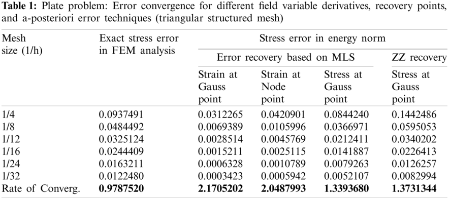
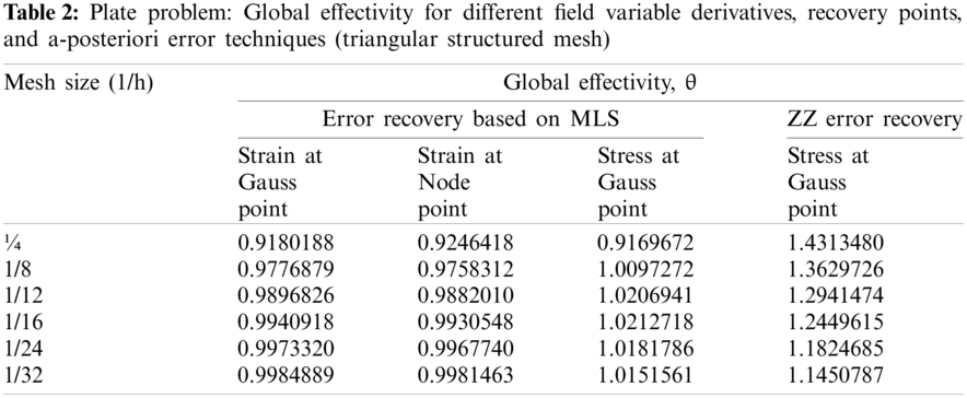
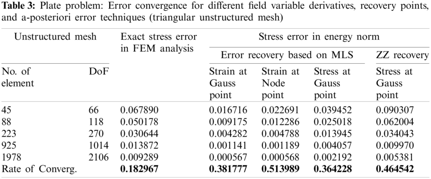
where constants α and β are given by the relations as α=[E.ν/((1−2.ν)⋅(1+ν))], β=[E/(2.(1+ν))], and E and ν are Modulus of elasticity and Poisson’s Ratio respectively with a value of 1.0 N/mm2 and 0.3.

The linear quadrilateral element and triangular element meshing scheme are used to discretize the plate domain in structured as well as unstructured manner. Fig. 2 shows employed meshing scheme for domain discretization in finite element analysis. The error convergence with mesh-refinement in finite-element solution and, recovered solution for derivatives of state variable at Gauss/node points using MLS based a-posteriori error technique are given in Tabs. 1, 3, 5 and 7 for different discretization scheme respectively. The global effectivity of error estimation for different discretization scheme obtained is presented in Tabs. 2, 4, 6 and 8. The error estimation results using patch based ZZ recovery technique are also presented in Tabs. 1 to 8 with different discretization schemes. The element (local) effectivity frequency is also calculated using different structured/unstructured discretization schemes at Gauss/node points. The element effectivity frequency is portrayed in Figs. 3 and 4, at last refinement level, for comparison of performance with different recovery parameters, i.e., Gauss/node points and field variable derivative recovery. The stress error distribution in plate domain for different recovered field variables derivatives using different discretization scheme, at gauss/node points are plotted in Figs. 5 and 6.

The elastic plate with circular hole, a typical stress concentration problem under the action of a unit in-plane traction applied in the x-direction, is tested for MLS interpolation based recovery method effectivity and convergence characteristics. The plate side is 5a, having radius of the circular hole “a” as 1. The vertical, and normal displacement components are zero along the circular arc of quarter part of circular hole plate. Along the symmetry lines of circular hole plate, the shear stress is zero. The known close form stress field solutions are given in Eqs. (30) to (32) [8].

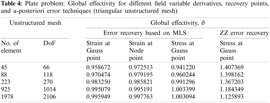
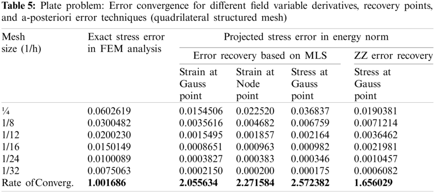
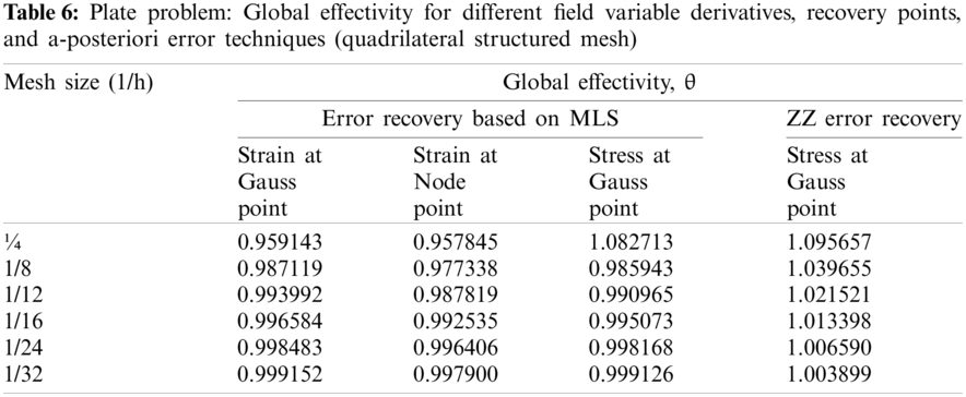
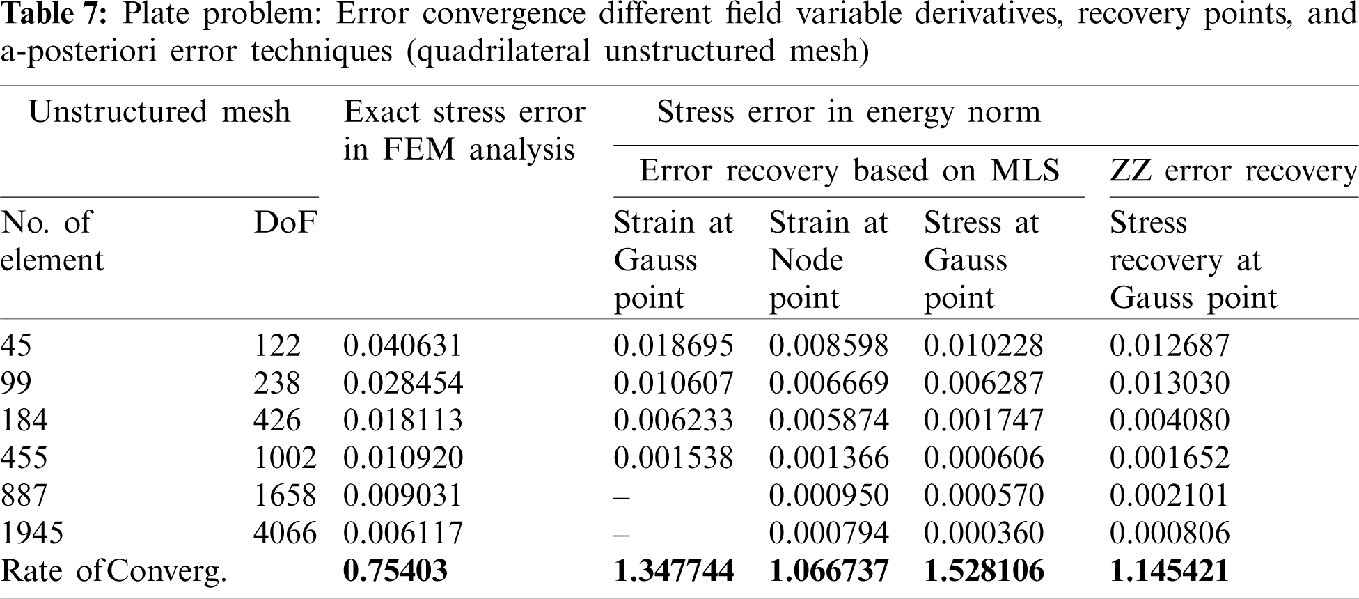
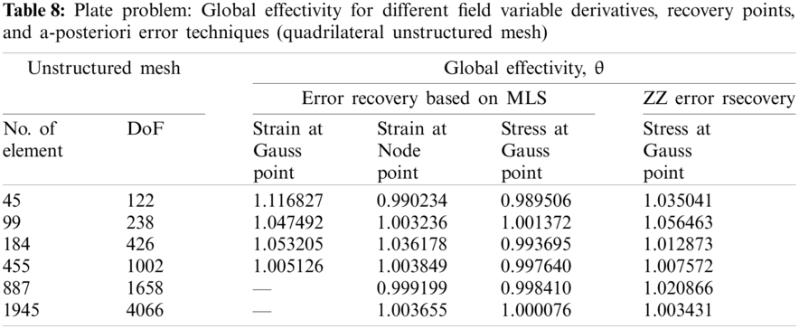
Figure 3: Plate problem: Local effectivity vs. number of elements in plate problem for different field variable derivatives, recovery points, and a-posteriori error techniques (triangular mesh) (i) structured mesh size (h) = 1/32 (ii) elements in unstructured mesh = 1978

Figure 4: Plate problem: Local effectivity vs. number of elements for different field variable derivatives, recovery points, and a-posteriori error techniques (quadrilateral mesh) (i) structured mesh size (h) = 1/32 (ii) elements in unstructured mesh = 455

Figure 5: Error distribution in plate problem domain in plate problem for different field variable derivatives, recovery points, and a-posteriori error techniques [triangular mesh size (h) = 1/32] (a) exact error (b) projected error (ZZ, stress at gauss point) (c) projected error (MLS based strain at Gauss point) (d) projected error (MLS based strain at Node point) (e) projected error (MLS based stress at Gauss point)

Figure 6: Error distribution in plate problem domain for different field variable derivatives, recovery points, and a-posteriori error techniques [quadrilateral mesh size (h) = 1/32] (a) exact error (b) projected error (ZZ, stress at Gauss point) (c) projected error (MLS based strain at Gauss point) (d) projected error (MLS based strain at Node point) (e) projected error (MLS based stress at Gauss point)

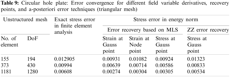
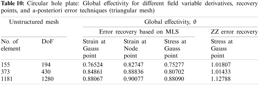
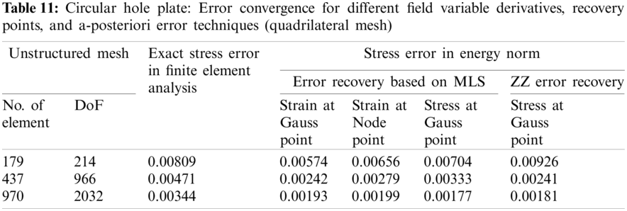
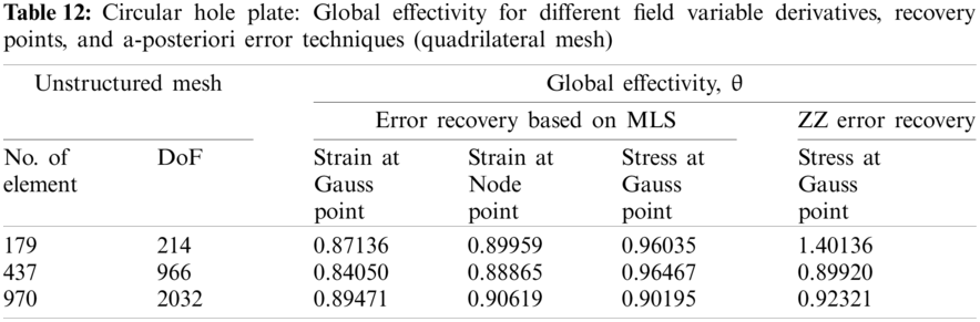
The one quarter of circular hole plate domain is modeled because of symmetry of plate problem. and domain is discretized with linear triangular/quadrilateral elements as shown in Fig. 7. The error convergence with order of refinement in finite element solution and, recovered solution for derivatives of state variable at Gauss/node points using MLS based a-posteriori error technique and ZZ recovery technique are represented in Tabs. 9 and 11 for different discretization scheme, respectively. The effectivity (global) of error estimation acquired with MLS based a-posteriori error technique and ZZ recovery technique for different discretization scheme is given in Tabs. 10 and 12. The local or element effectivity frequency in plate domain is also found using different recovery parameters and is portrayed in Fig. 8 at last mesh level considered.

The study compares the MLS based technique and Zienkiewicz-Zhu (ZZ) technique used a-posteriori in finite element analysis by analyzing benchmark problems, i.e., square solid plate and plate with circular hole in elastic framework. The performance of recovery techniques is studied by varying recovery parameters, i.e., recovery points (Gauss/node) and recovered field variables derivatives (Strain/Stress). Four different discretization schemes namely, triangular, quadrilateral, structured and unstructured schemes are considered in the study. The MLS based a-posteriori error technique considers element free scattered nodes in support domain (a circular zone in the study) for post processing of the field variable derivatives, while Zienkiewicz-Zhu (ZZ) error estimation considers mesh dependent patch of elements surrounding the vertex node. The flow chart to show the adaptive finite element analysis using the recovery techniques is depicted in Fig. 9.

Numerical experiments with MLS based a-posteriori error technique demonstrate that the higher convergence and accuracy is obtained in recovered Gauss/node point values of the derivatives with different meshing schemes, and it is clear from Tabs. 1–8 that error recovery parameters, type of recovery points and field variables derivatives, affect the performance of MLS based error estimation. The solution errors in the finite element analysis, called discretization error, are crept due to subdivision of problem domain. The discretization errors are generated because the sub-domains are not capable of representing the full range of behavior of the continuum. The discretization error can be decreased by finer elements mesh. The MLS based a-posteriori error technique performs better with quadrilateral elements discretization as compared to domain discretization with triangular elements. The MLS interpolation based recovery technique performs better for stress extraction at Gauss points with quadrilateral discretization of problem domain. However, for triangular discretization of problem domain, the MLS interpolation based recovery technique performs better for strain extraction at node points. This is also verified with Fig. 3 and it shows element effectivity frequency in plate domain. The figure infers that local effectivity is converging to around one for most of the elements for stress recovery at Gauss point using the MLS based a-posteriori error technique. Exact and computed error distributions using different discretization scheme, recovery points and recovered field variables, displayed in Figs. 5 and 6, supports the conclusions for better performance of MLS based recovery technique stress extraction at gauss points. It concludes that MLS based a-posteriori error technique effectively predicts the error in energy norm of the recovered solution for stress both at local and global levels.

Figure 8: Circular hole plate: Local effectivity vs. number of elements for different field variable derivatives, recovery points, and a-posteriori error techniques (a) triangular mesh (elements = 1002) (b) quadrilateral mesh (elements = 358)

Figure 9: Flow chart for ZZ and MLS recovery technique based adaptive finite element analysis

The error estimation incorporated finite element analysis results, shown in Tabs. 9–12 and Fig. 8, for circular hole plate with MLS interpolation and mesh dependent patch based a-posteriori error techniques, by varying discretization scheme, recovery points and field variables derivative recovery, also predict similar performance. It is also seen that MLS based a-posteriori error technique for extraction of field variable derivative is more effective than the mesh dependent patch based ZZ recovery technique especially with stress concentration problems. The poor performance of ZZ error recovery scheme may be due to inaccurate recovery of nodal derivatives and computed stresses on boundary as the number of sampling node in ZZ scheme will be lesser due to patch dependency on the meshing scheme. However, there is no mesh dependency for number of sampling nodes on boundary in the support domain, i.e., patch of influenced nodes within a determined distance. The error convergence is much faster with increasing order of meshing in MLS based a-posteriori error technique as compared to the finite element solution and ZZ technique based solution, so the cost of computation required to obtain a solution with a predefined accuracy will be smaller than for traditional h-adaptive processes.

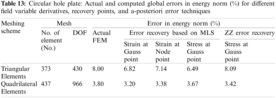
Adaptive analysis of plate problem, i.e., refinement of finite element mesh under guidance of a-posteriori error techniques for satisfying predefined error limit is also carried out. Adaptive analysis results are obtained for ZZ error recovery and MLS based a-posteriori error technique with different discretization scheme, recovery point and recovered field variable derivatives. The initial meshes are adaptively modified to bring the solution error within the target limit. Tabs. 13 and 14 show the degrees of freedom and number of elements in refined meshes at prescribed error limit of 2%. Figs. 10–11 show the adaptively improved meshes through the guidance of ZZ error recovery and MLS based a-posteriori error technique for triangular and quadrilateral meshing schemes. It is clear from the figures of adaptively refined meshes that the initial uniform mesh become high density mesh in field variable derivative concentration area, i.e., near the plate hole and low density mesh away from the plate hole. However, the mesh is uniformly dense near the hole using the quadrilateral element mesh as compared to the density mesh generated using the triangular element mesh. It can be concluded that domain discretization using quadrilateral element is more effective and faithful to recover the field variable derivative errors. The MLS based a-posteriori error technique coupled adaptive analysis found that the number of elements required to achieve target accuracy with stress extraction at Gauss point is lesser as compared to strain extraction at Gauss or node point. It infers that the MLS based a-posteriori error technique is more efficient in extracting the stresses at Gauss point as compared to the extraction of strains. Also, lesser number of elements are required to achieve target accuracy using the MLS based a-posteriori error technique as compared to patch based ZZ error estimation with quadrilateral meshing schemes and number of elements using the MLS based a-posteriori error technique are comparable with triangular meshing schemes. It concludes that MLS based a-posteriori error technique is more efficient than the ZZ recovery technique.

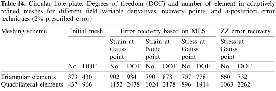
Figure 10: Circular hole plate: Adaptively refined mesh for different field variable derivatives, recovery points with ZZ & MLS a-posteriori error techniques [triangular initial mesh elements = 373, 2% prescribed error] (a) initial mesh (b) stress (ZZ, Gauss) (c) strain (Gauss) (d) strain (Node) (e) stress (Gauss)

Figure 11: Circular hole plate: Adaptively refined mesh for different field variable derivatives, recovery points with ZZ & MLS a-posteriori error techniques [quadrilateral initial mesh elements = 437, 2% prescribed error] (a) initial mesh (b) stress (ZZ, Gauss) (c) strain (Gauss) (d) strain (Node) (e) stress (Gauss)

The study presents the effectiveness of moving least squares (MLS) interpolation based on a-posteriori error technique to recover the finite element solution error with varying the finite element error recovery parameters, namely types of recovery points and field variable derivatives recovery. The MLS technique has a limitation: it needs a dilation factor to form a proper patch size and requires a proper order of basis function for a particular problem. The moment matrix of MLS technique may result in ill-conditioning or singular due to inappropriate nodes distribution and polynomial basis functions. Moreover, the Kronecker delta function property is not satisfied in MLS based technique. Special measures such as Lagrange multiplier methods, penalty method etc., are required to impose essential boundary conditions in the elastic analysis. The MLS interpolation based a-posteriori technique uses the weighted least squares method on top of the finite element method's field variable derivatives solution to build a continuous field variable derivatives approximation. The stress and strains are recovered at two kinds of recovery points, i.e., at Gauss points (at super-convergent stress locations) and nodal points. The numerical tests consider discretization with quadrilateral and triangular meshes to measure the approximation errors in strain and stress fields. The numerical examples showed capabilities of the MLS interpolation based recovery technique for effective error estimation in the finite element analysis. The higher convergence and improved behavior of MLS interpolation based a-posteriori error technique is achieved for stresses recovered at Gauss point compared to strains recovered at Gauss/node point using quadrilateral elements discretization. The MLS-based a-posteriori error technique coupled adaptive analysis found that fewer elements are required to achieve target accuracy with stress extraction at Gauss point compared to strain extraction at Gauss or node point. The MLS interpolation based recovery technique performs better for stress extraction at Gauss points with a quadrilateral discretization of problem domain. In contrast, the recovery technique performs better for strain extraction at node points for the triangular discretization of problem domain. The study also concluded that MLS interpolation based a-posteriori technique is more effective and efficient than the mesh dependent ZZ recovery technique.

Funding Statement:The authors extend their appreciation to the Deanship of Scientific Research at King Khalid University for funding this work through General Research Project under Grant No. (R.G.P2/73/41). The authors also acknowledge to the Dean, Faculty of Engineering for his valuable support and help.

Conflicts of Interest:The authors declare that they have no conflicts of interest to report regarding the present study.

References

1. Taus, M., Rodin, G. J., Hughes, T. R., Scott, M. A. (2019). Isogeometric boundary element methods and patch tests for linear elastic problems: Formulation, numerical integration, and applications. Computer Methods in Applied Mechanics and Engineering, 357, 112591. DOI 10.1016/j.cma.2019.112591. [Google Scholar] [CrossRef]

2. Zienkiewicz, O. C. (2000). Achievement and some unsolved problems of finite element method. International Journal for Numerical Methods in Engineering, 47(1–3), 9–28. DOI 10.1002/(SICI)1097-0207(20000110/30)47:1/33.0.CO;2-P. [Google Scholar] [CrossRef]

3. Chen, J. S., Hillman, M. M., Chi, S. W. (2017). Mesh free methods: Progress made after 20 ysears. Journal of Engineering Mechanics, 143(4), 4017001. DOI 10.1061/(ASCE)EM.1943-7889.0001176. [Google Scholar] [CrossRef]

4. Zhang, T., Li, X. (2020). Analysis of the element-free Galerkin method with penalty for general second-order elliptic problems. Applied Mathematics and Computation, 380, 125306. DOI 10.1016/j.amc.2020.125306. [Google Scholar] [CrossRef]

5. Li, X., Dong, H. (2021). An element-free Galerkin method for the obstacle problem. Applied Mathematics Letters, 112, 106724. DOI 10.1016/j.aml.2020.106724. [Google Scholar] [CrossRef]

6. Cen, S., Wu, C. J., Li, Z., Shang, Y., Li, C. (2019). Some advances in high-performance finite element methods. Engineering Computations, 36(8), 2811–2834. DOI 10.1108/EC-10-2018-0479. [Google Scholar] [CrossRef]

7. Zienkiewicz, O. C., Zhu, J. Z. (1987). Simple error estimator and adaptive procedure for practical engineering analysis. International Journal for Numerical Methods in Engineering, 24(2), 337–357. DOI 10.1002/nme.1620240206. [Google Scholar] [CrossRef]

8. Zienkiewicz, O. C., Zhu, J. Z. (1992). The super-convergent patch recovery and a-posteriori error estimates. Part I, the a-posteriori error technique. International Journal for Numerical Methods in Engineering, 33(7), 1331–1364. DOI 10.1002/nme.1620330702. [Google Scholar] [CrossRef]

9. Niu, Q., Shephard, M. S. (1993). Super-convergent extraction techniques for finite element analysis. International Journal for Numerical Methods in Engineering, 36(5), 811–836. DOI 10.1002/nme.1620360507. [Google Scholar] [CrossRef]

10. Ubertini, F. (2004). Patch recovery based on complementary energy. International Journal for Numerical Methods in Engineering, 59(11), 1501–1538. DOI 10.1002/nme.924. [Google Scholar] [CrossRef]

11. Rodenas, J. J., Tur, M., Fuenmayor, F. J., Vercher, A. (2007). Improvement of the super-convergent patch recovery technique by the use of constraint equations: The SPR-C technique. International Journal for Numerical Methods in Engineering, 70(6), 705–727. DOI 10.1002/nme.1903. [Google Scholar] [CrossRef]

12. Kim, K., Lee, H. (2010). A posteriori error estimator for non-conforming finite element methods of the linear elasticity problem. Journal of Computational and Applied Mathematics, 235, 186–202. DOI 10.1016/j.cam.2010.05.032. [Google Scholar] [CrossRef]

13. Mohite, P. M., Upadhyay, C. S. (2015). Adaptive finite element based shape optimization in laminated composite plates. Computers and Structures, 153, 19–35. DOI 10.1016/j.compstruc.2015.02.020. [Google Scholar] [CrossRef]

14. Ródenas, J. J., González-Estrada, O. A., Fuenmayor, F. J., Chinesta, F. (2013). Enhanced error estimator based on a nearly equilibrated moving least squares recovery technique for FEM and XFEM. Computational Mechanics, 52(2), 321–344. DOI 10.1007/s00466-012-0814-7. [Google Scholar] [CrossRef]

15. Parret-Fréaud, A., Rey, V., Gosselet, P., Rey, C. (2016). Improved recovery of admissible stress in domain decomposition methods—Application to heterogeneous structures and new error bounds for FETI-DP. International Journal for Numerical Methods in Engineering, 111(1), 69–87. DOI 10.1002/nme.5462. [Google Scholar] [CrossRef]

16. Sharma, R., Zhang, J., Langelaar, M., van Keulen, F., Aragón, A. M. (2018). An improved stress recovery technique for low-order 3D finite elements. International Journal for Numerical Methods in Engineering, 114, 88–103. DOI 10.1002/nme.5734. [Google Scholar] [CrossRef]

17. Breitkopf, P., Rassineux, A., Villon, P. (2002). An introduction to moving least squares meshfree methods. Revue Européenne des Eléments, 11(7–8), 825–867. DOI 10.3166/reef.11.825-867. [Google Scholar] [CrossRef]

18. Sukumar, N., Moran, B., Black, T., Belytschko, T. (1997). An element-free Galerkin method for three-dimensional fracture mechanics. Computational Mechanics, 20, 170–175. DOI 10.1007/s004660050235. [Google Scholar] [CrossRef]

19. Cai, D., Cai, Z. (2018). A hybrid a posteriori error estimator for conforming finite element approximations. Computer Methods in Applied Mechanics and Engineering, 339, 320–340. DOI 10.1016/j.cma.2018.04.050. [Google Scholar] [CrossRef]

20. Dong, Y., Yuan, S., Xing, Q. (2019). Adaptive finite element analysis with local mesh refinement based on a posteriori error estimate of element energy projection technique. Engineering Computations, 36(6), 2010–2033. DOI 10.1108/EC-11-2018-0523. [Google Scholar] [CrossRef]

21. Ullah, Z., Coombs, W. M., Augarde, C. E. (2013). An adaptive finite element/meshless coupled method based on local maximum entropy shape functions for linear and nonlinear problems. Computer Methods in Applied Mechanics and Engineering, 267, 111–132. DOI 10.1016/j.cma.2013.07.018. [Google Scholar] [CrossRef]

22. Chung, H. J., Belytschko, T. (1998). An error estimate in the EFG method. Computational Mechanics, 21, 91–100. DOI 10.1007/s004660050286. [Google Scholar] [CrossRef]

23. Kumar, S., Fourment, L., Guerdoux, S. (2015). Parallel, second-order and consistent remeshing transfer operators for evolving meshes with super-convergence property on surface and volume. Finite Elements in Analysis and Design, 93, 70–84. DOI 10.1016/j.finel.2014.09.002. [Google Scholar] [CrossRef]

24. Ahmed, M. (2020). A comparative study of mesh-free radial point interpolation method and moving least squares method-based error estimation in elastic finite element analysis. Arabian Journal for Science and Engineering, 45, 3541–3557. DOI 10.1007/s13369-019-04154-5. [Google Scholar] [CrossRef]

25. Ahmed, M., Hechmi, M., Singh, D., Kahla, N. B. (2019). A parametric study of mesh free interpolation based recovery techniques in finite element elastic analysis. Computer Modeling in Engineering & Sciences, 121(2), 687–786. DOI 10.32604/cmes.2019.06886. [Google Scholar] [CrossRef]

26. Liu, G. R. (2003). MFree shape function construction. Mesh free methods—moving beyond the fnite element method. Boca Ratón: CRC Press. [Google Scholar]

27. Liu, G. R. (2016). An overview on meshfree methods: For computational solid mechanics. International Journal of Computational Methods, 13(5), 1630001–1630042. DOI 10.1142/S0219876216300014. [Google Scholar] [CrossRef]

28. Lin, H., Atluri, S. N. (2000). Meshless local Petrov-Galerkin (MLPG) method for convection-diffusion problems. Computer Modelling in Engineering & Sciences, 1(2), 45–60. DOI 10.3970/cmes.2000.001.205. [Google Scholar] [CrossRef]