Quantile Version of Mathai-Haubold Entropy of Order Statistics

Ibrahim Almanjahie; Javid Dar; Amer Al-Omari; Aijaz Mir

doi:10.32604/cmes.2021.014896

Ibrahim M. Almanjahie1,2,*, Javid Gani Dar3, Amer Ibrahim Al-Omari4 and Aijaz Mir5

1Department of Mathematics, College of Science, King Khalid University, Abha, 62529, Saudi Arabia
2Statistical Research and Studies Support Unit, King Khalid University, Abha, 62529, Saudi Arabia
3Department of Mathematical Sciences, IUST, Kashmir, 192231, India
4Department of Mathematics, Faculty of Science, Al al-Bayt University, Mafraq, 25113, Jordan
5Department of Mathematics, Govt. Degree College Kilam, Higher Education, J & K, 192231, India
*Corresponding Author: Ibrahim M. Almanjahie. Email: imalmanjahi@kku.edu.sa
Received: 06 November 2020; Accepted: 18 March 2021

Abstract: Many researchers measure the uncertainty of a random variable using quantile-based entropy techniques. These techniques are useful in engineering applications and have some exceptional characteristics than their distribution function method. Considering order statistics, the key focus of this article is to propose new quantile-based Mathai-Haubold entropy and investigate its characteristics. The divergence measure of the Mathai-Haubold is also considered and some of its properties are established. Further, based on order statistics, we propose the residual entropy of the quantile-based Mathai-Haubold and some of its property results are proved. The performance of the proposed quantile-based Mathai-Haubold entropy is investigated by simulation studies. Finally, a real data application is used to compare our proposed quantile-based entropy to the existing quantile entropies. The results reveal the outperformance of our proposed entropy to the other entropies.

Keywords: Shannon entropy; Mathai-Haubold entropy; quantile function; residual entropy; order statistics; failure time; reliability measures

The order statistics are considered in a varied scope of complicated problems, including characterization of a probability distribution, quality control, robust statistical estimation and identifying outliers, analysis of a censored sample, the goodness of fit-tests, etc. Based on order statistics, the usage of the recurrence relationships for moments is well recognized by many researchers (see, for instance, Arnold et al. [1], Malik et al. [2]). For an enhancement, many recurrence relations and identities for the order statistics moments originating from numerous particular continuous probability distributions (i.e., gamma, Cauchy, normal, logistic, and exponential) have been reviewed by Samuel et al. [3] and Arnold et al. [1].

Based on a random sample of X1,X2,…,Xn, let the corresponding order statistics to be X1:n≤X2:n≤…≤Xn:n. Then, as in David [4] and Arnold et al. [1], the density of Xr:n,1≤r≤n, is

with Cr:n=n!(r−1)!(n−r)!. Eq. (1) can be used to determine the smallest (when r=1) and largest (when r=n) probability density functions; they, respectively, are f(1,n)(x)=n[1−F(x)]n−1f(x) and f(n,n)(x)=n[F(x)]n−1f(x). The corresponding distribution functions are obtained, respectively, by F(1,n)(x)=1−[1−F(x)]n and F(n,n)(x)=[F(x)]n.

Shannon [5] was the first author who introduced the entropy idea for a random variable (r.v.) X in the field of information theory and defined it as

Here, fX(x) indicates the pdf of the r.v. X. Based on the Shannon entropy measure, Mathi et al. [6] (now onwards M-H entropy) developed a generalized version of Eq. (2) and defined it as

When α→1 the M-H entropy measure Mα(X) will be reduced to the Shannon entropy measure defined in Eq. (2).

Mathai et al. [6] and Sebastian [7] discussed the main property allied with Eq. (3). In other words, applying the maximum entropy and using its normalization version together with energy restrictions will result in the well-recognized pathway-model as provided by Mathai [8]. However, this model contains many special cases of familiar probability distributions.

Theoretical surveys and applications employing the measurement information are distributional dependents, and they may be found to be not appropriate in circumstances once the distribution is analytically not tractable. Hence, utilizations of quantile function are considered as an alternative method, where

We refer the readers to Nair et al. [9] and Sunoj et al. [10] and references therein for more details about quantile function. Recently, Sunoj et al. [11] studied Shannon entropy and as well as its residual and introduced quantile versions of them defined as

respectively, where q(u)=dQ(u)du denotes the density of quantile function. If we define the quantile density function by fQ(u)=f(Q(u)), then, we obtain

For Shannon past entropy, Sunoj et al. [11] also introduced its quantile version and defined it as

In the present paper, we work with the order statistics, propose the quantile-based version of M-H entropy and discuss its properties. The M-H divergence measure is also considered and we establish some of its distribution free properties. In addition, we introduce the version of the quantile-based residual for the M-H entropy and prove some characterization results. To the best of our knowledge, the results presented here, treat a research gap that has not been addressed or studied systematically by others, which was the primary motivation of our paper.

The paper is outlined as follows. Section 2 is devoted to the construction of our quantile-based M-H entropy and its properties. Next, expressions for the quantile-based version of M-H entropy for some life-time distributions are presented in Section 3. A quantile-based generalized divergence measure of rth order statistics is given in Section 4. Quantile Residual Entropy of M-H for rth order statistics and also for some lifetime models are introduced in Section 5. Characterization theorems based on M-H Quantile Residual Entropy are presented in Section 6. In Section 7, simulation studies for investigating the performance of our proposed quantiles and real data life application are presented. Our conclusion is stated in Section 8.

Wong et al. [12], Park [13], Ebrahimi et al. [14] and Baratpour et al. [15] are the authors who discuss in detail the aspects of information-theoretic based on order statistics. Paul et al. [16] considered the M-H entropy and, based on record values, studied some of its essential properties. For rth order statistics Xr;n, the M-H entropy is defined as

where fr;n(x) is given in Eq. (1). Now, FQ(u)=u, then, the pdf of rth order statistics becomes

where gr(u) denotes beta-distribution density with r and (n−r+1) as its parameters. The quantile-based M-H entropy of Xr;n is determined by

MXr:nα=MXr:nα(Q(u))=1α−1(∫01fr:n2−α(Q(u))d(Q(u))−1)=1α−1(∫01(gr(u))2−α(q(u))α−1du−1) (6)

which is the quantile entropy of rth order statistics investigated by Sunoj et al. [10].

In the following, we provide expressions for Quantile-based M-H entropy of order statistics for some life time distributions:

(i) Govindarajulu’s Distribution: The quantile version and the corresponding density functions, respectively, are

Using Eq. (6), we can easily obtain quantile-based M-H Entropy of rth order statistics for Govindarajulu distribution as

Similarly, based on the quantile and quantile density functions, we obtain the quantile-based for the M-H Entropy (MXr:nα) of rth order statistics for the following distributions.

Figs. 1–3 give the quantile version of M-H entropy plots of smallest order statistics under exponential, Pareto-I and uniform distributions, respectively.

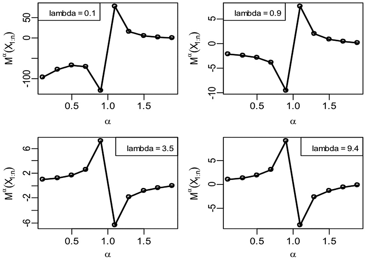
Figure 1: Quantile M-H entropy plots of smallest order statistics (Exponential distribution)

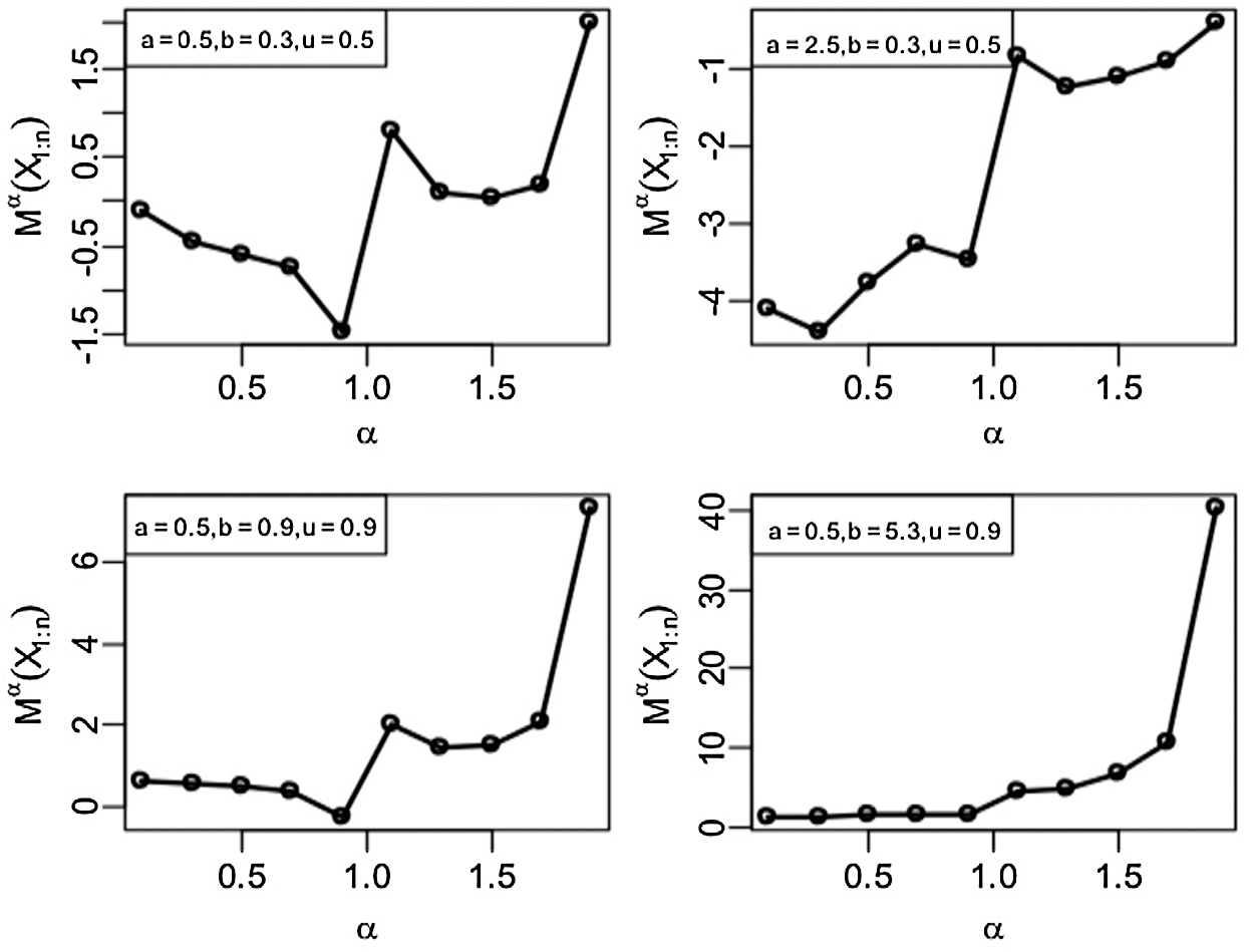
Figure 2: Quantile M-H entropy plots of smallest order statistics (Pareto-I Distribution)

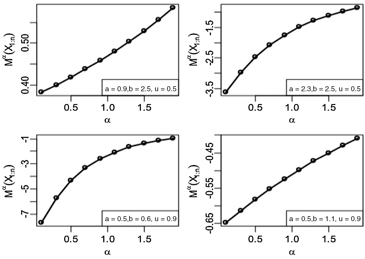
For an increasing value of parameters α and λ, the entropy plot, based on the exponential distribution, increases. In the case of entropy plot under the Pareto-I distribution, the plot has an increasing (a decreasing) behaviour for different parameter combinations. The entropy plot under uniform distribution also has increasing behaviour for different parameter values. Tabs. 1--3 give entropy values when the parameters α and λ are varied.

Figure 3: Quantile M-H entropy plots of smallest order statistics (Uniform Distribution)

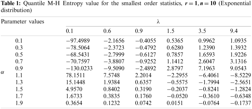
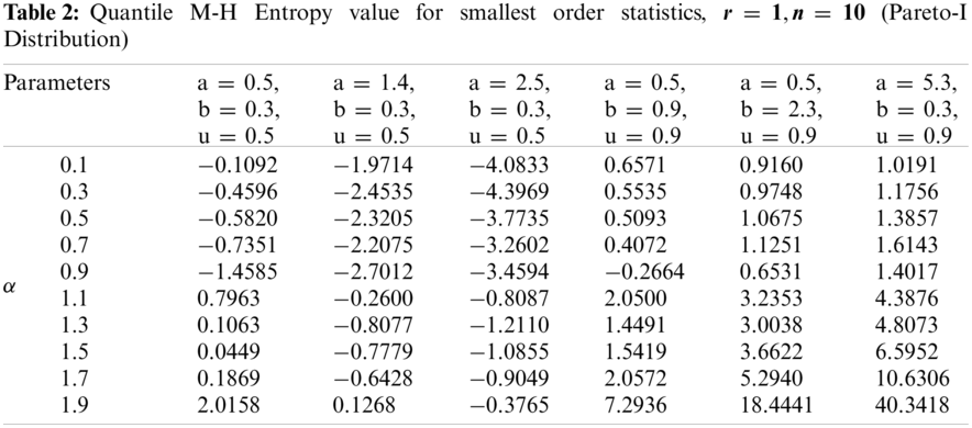
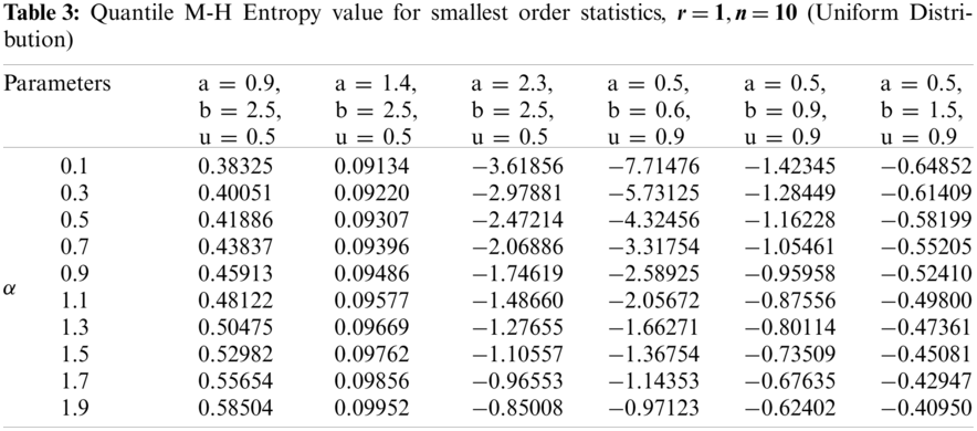
Clearly, we see from Tabs. 1–3 that the entropy values under exponential, Pareto-I and uniform distributions portray the same behaviour as discussed in the graphical plots.

Different measures deal with the dissimilarity or the distance between two probability distributions. Certainly, these measures are essential in theory, inferential statistics, applied statistics and data processing sciences, such as comparison, classification, estimation, etc.

Assume f and g are the density functions of the non-negative r.vs X and Y, respectively. The direct divergence of f from g is measured by the Kullback et al. [17] and is

With order α, the divergence measure of the M-H or the relative-entropy of g concerning f is obtained by

where, for α→1, the expression in Eq. (8) reduces to Eq. (7) (see Kullback et al. [17]).

Theorem 4.1: The quantile-based-generalized divergence measure between the rth order statistics distribution and the primary distribution is a distribution-free.

Now, using the value of fr:n(x) in Eq. (9), we obtain Mα(Xr:n/X)=11−α{∫0∞F(2−α)(r−1)(x)(1−F(x))(n−r)(2−α)(β(r,n−r+1))2−αf(x)dx−1}.

Using the fact that q(u)f(Q(u))=1, we determine the quantile-based-generalized divergence measure between the distribution of rth order statistics and primary distribution, as

Entropy functions are very popular in the applications of finance and tectonophysics, machine learning, reliability theory, etc. However, in reliability and real-life applications, the life test time is truncated at a specific time, and in such situations, Eq. (2) is not an appropriate measure. Therefore, Shannon's entropy is not an adequate measure when we have knowledge about the component's current age, which can be used when determining its uncertainty. Ebrahimi [14] describes a more practical approach that considers the use of age, defined as

with F¯(t) indicates the survival-function. Note that for t=0, the Eq. (5) reduces to Eq. (4). Denote by X, a non-negative r.v., the unit’s life-time at time t. Then, the residual function of M-H [18] is

where F¯r;n(x)=β¯x(r,n−r+1)β(r,n−r+1) refers to the survival-function of the rth order statistics and β¯x(r,n−r+1) is the incomplete gamma function.

Considering the rth order statistic, the quantile residual entropy function of M-H of is given by

Mα(Xr;n;u)=Mα(Xr;n;Q(u))=1α−1{(β(r,n−r+1))2−α(β¯u(r,n−r+1))2−α∫u1gr2−α(p)qα−1(p)dp−1}. (10)

Theorem 5.1: Considering the rth order statistic, the quantile residual entropy function of M-H determines the underlying distribution uniquely.

where ′ denotes the differentiation w.r.t u. This equation involved an immediate connection between the q(u) and Mα(Xr;n;u), which implies that the quantile residual entropy function of M-H of rth order statistic leads to the unicity of the underlying distribution.

Next, we make the derivation of the quantile form of M-H residual entropy of the rth order statistic for some lifetime models.

The quantile residual entropy function of M-H of rth order statistics for the distribution of Govindarajulu is

Similarly, based on the quantile and quantile density functions, we obtain the quantile-based residual M-H Entropy of rth order statistics for the following distributions.

(iv) Exponential distribution Q(u)=−log⁡(1−u)λ and q(u)=1λ(1−u),0≤u<1; λ>0.

Based on residual M-H quantile entropy of order statistics Mα(Xr;n,u), the following nonparametric classes of life distribution are defined.

Definition 5.1: X is said to have an increasing (a decreasing) M-H quantile entropy of order statistics if Mα(Xr;n,u) is increasing (decreasing) in u≥0.

The following lemma is useful in proving the results in monotonicity of Mα(Xr;n,u).

Lemma 5.1: Let f(u,x):R+2→R+ and g:R+→R+ be any two functions. If ∫u∞f(u,x)dx is increasing and g(u) is increasing (decreasing) in u, then ∫u∞f(u,x)g(x)dx is increasing (decreasing) in u, provided the existence of integrals.

Theorem 5.2: Let X be a non-negative and continuous r.v. with quantile QX(.) and density qX(.). Define Y=∅(X), where ∅(.) is nonnegative, increasing and convex(concave) function. Then,

(i) For 1<α<2, Mα(Yr;n,u) increases (or decreases) in u whenever Mα(Xr;n,u) increases (or decreases) in u.

(ii) For 0<α<1, Mα(Yr;n,u) increases (or decreases) in u whenever Mα(Xr;n,u) increases (or decreases) in u.

Proof: (i) The quantile density of Y is given by g(QY(u))=1qY(u)=1qX(u)∅′(QX(u)).

Mα(Yr;n;u)=1α−1{(β(r,n−r+1))2−α(β¯u(r,n−r+1))2−α∫u1gr2−α(p)(qX(p)∅′(QX(p)))α−1dp−1} (11)

Since 1<α<2 and ∅ is non-negative, increasing and convex (concave) function, the (∅′(QX(p))α−1 increases (or decreases) and it is also non-negative. Consequently, using Lemma 3.1, Eq. (11) is increasing (decreasing), which gives the proof of (i) of the Theorem. Similarly, 0<α<1, (∅′(QX(p))α−1 increases (or decreases) in p, because ∅ increases and it is convex. Consequently, Eq. (11) is decreasing (increasing) in u, which proves (ii) of the Theorem. The immediate application of Theorem 5.2 is given below:

Let X be an r.v. following the distribution of exponential and having a failure rate λ. Also, let Y=X1α,α>0. Therefore, Y follows Weibull distribution where Q(u)=λ−1α(−log⁡(1−u))1α. The function ϕ(x)=x1α,x>0,α>0 is a convex (concave) if 1<α<2,(0<α<1). Hence, based on Theorem 5.2, the Weibull distribution is increasing (decreasing) M-H quantile entropy of order statistics if 1<α<2,(0<α<1).

This section provides some characterizations for the quantile M-H residual entropies of the smallest and largest order statistics. The corresponding quantile M-H residual entropy can be determined by substituting r=1 (for smallest) and r=n (for largest) in Eq. (10) and are, respectively, given by

Mα(X1;n;u)=Mα(X1;n;Q(u))=1α−1{n2−α(1−u)n(2−α)∫u1g12−α(p)qα−1(p)dp−1} (12)

Now, we define the hazard and the reversed hazard functions for the quantile version which are, respectively, corresponding to the well-recognized hazard rate and reversed hazard rate functions, as K(u)=h(Q(u))=fQ(u)(1−u)=1(1−u)q(u) and K¯(u)=K¯(Q(u))=fQ(u)F(Q(u))=(uq(u))−1.

In numerous practical circumstances, the uncertainty is essentially not identified with the future. Therefore, it can likewise allude to the past. This thought empowered Crescenzo et al. [19] to build up the idea of past entropy on (0,t). If X denotes the life-time of a component, thus, the past entropy of X is obtained by

with F(t) is the cumulative distribution function. For t=0, Eq. (13) reduces to Eq. (2).

The quantile form of past M-H residual entropy of rth order statistic is determined by

M¯α(Xn;n;u)=1α−1{n2(2−α)(u)n(2−α)∫0up(2−α)(n−1)qα−1(p)dp−1}. (14)

Next, we state some properties based on quantile M-H residual entropy of the smallest order statistics.

Theorem 6.1: Let X1;n represents the first order statistics with survival and hazard quantile functions F¯1;n(x) and KX1;n(u). Then, the Mα(X1;n;u) is determined by

(ii) X follows Pareto distribution where the quantile density function is q(u)=ba{(1−u)−(1+1a)},0≤u≤1; a,b>0 if C<12−α.

(iii) X follows a finite range distribution with quantile density function q(u)=ba{(1−u)(1a−1)},0≤u≤1; b>0,a>1 if C>12−α.

Proof: Assume that the conditions in Eq. (15) are held. Then, using Eq. (12), we have

n2−α(1−u)n(2−α)∫u1(1−p)(2−α)(n−1)qα−1(p)dp=C(KX1;n(u))1−α. (16)

Therefore, using KX1;n(u)=n(1−u)q(u) in Eq. (16), then, differentiating (w.r.t) u, we obtain

This implies q(u)=A(1−u)n(2c−cα−1c−αc−1), where A is a constant. Thus, X has exponential distribution, Pareto distribution and finite range distribution if C=12−α,C<12−α,C>12−α, respectively.

Theorem 6.2: For the exponential distribution, the difference between quantile-based M-H residual entropy of the life-time of the series system (Mα(X1;n;u)) and M-H residual quantile entropy of the life-time of each component (Mα(X;u)) is independent of u and relies only on α and the number of components of the system.

Theorem 6.3: Let Xn;n represents the largest order statistics with hazard and survival quantile functions, K¯Xn;n(u) and F¯n;n(x). Then, for sample maxima Xn;n, the past quantile entropy of M-H, M¯α(Xn;n;u), is

Proof: The quantile and quantile density functions for the power distribution are, respectively,

It is simple to show that K¯Xn;n(u)=nbu1ba. Taking C=bn3−α2nb−nbα+α−1 gives the if part of Theorem.

Substituting K¯Xn;n(u)=nuq(u), we have {n3−α∫0up(2−α)(n−1)qα−1(p)dp}=Cu2n−nα+α−1(q(u))α−1.

Taken the derivative (w.r.t) u yields q′(u)q(u)=(n3−α−C(2n−nα+α−1)Cα−C)(1u). The latter gives

where A denotes a constant. Hence, the power distribution is a characterized for C=bn3−α2nb−nbα+α−1.

In this paper, the quantile-based M-H entropy is proposed for some distributions. However, based on the available real data and to keep the simulation study related to the application part, we investigate the performance of the quantile-based M-H entropy for the exponential distribution.

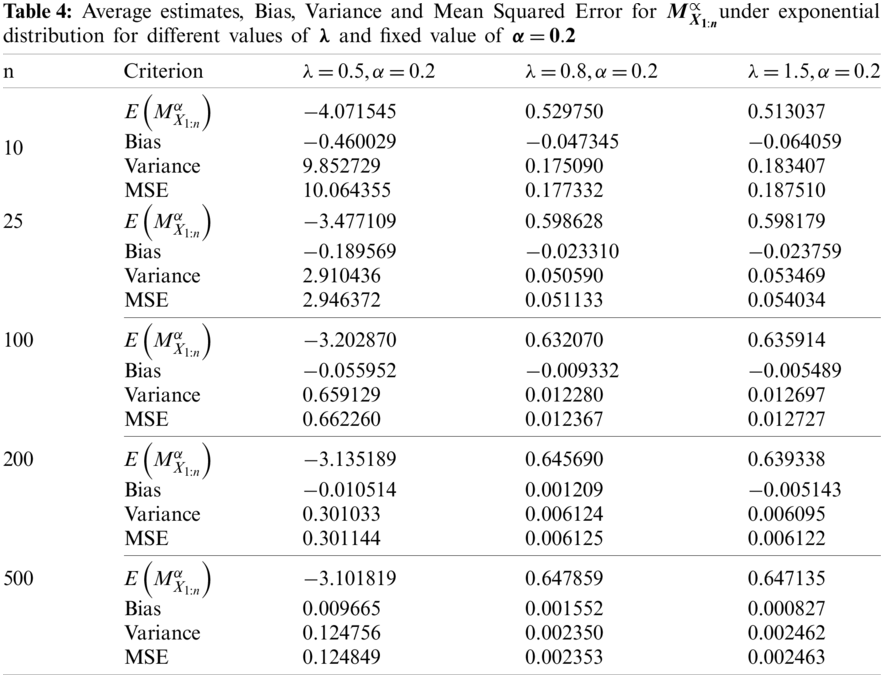
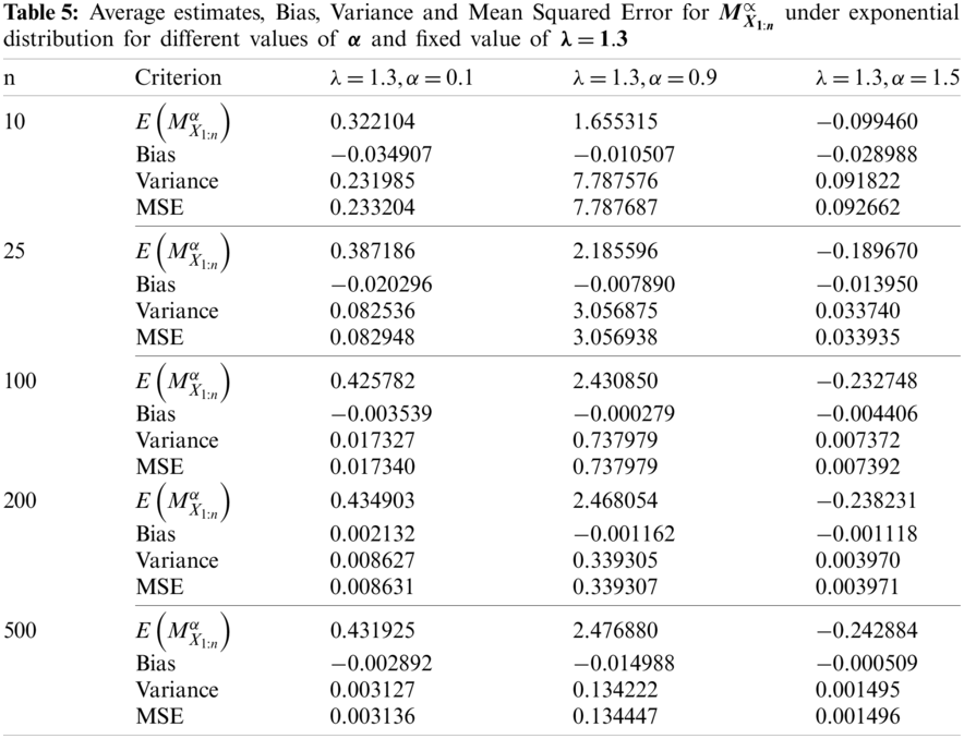
We conducted simulation studies to investigate the efficiency of the quantile-based M-H entropy estimators of smallest order statistics for exponential distribution (MX1:nα) in terms of the average bias (Bias), variance and mean squared error (MSE), based on sample sizes 10, 25, 100, 200 and 500 for different parameter combinations. The estimation of parameter λ was achieved using ML estimation and the process was repeated 2000 times.

From the results of the simulation study (see Tabs. 4 and 5), conclusions are drawn regarding the behaviour of the entropy estimator in general, which are summarized below:

1. The ML estimates of MX1:nα approaches to true value when sample size n increases.

The real data in this section represents the failure times of 20 mechanical components that were used previously by Murthy et al. [20] for investigating some of Weibull models. The data values are: 0.067, 0.068, 0.076, 0.081, 0.084, 0.085, 0.085, 0.086, 0.089, 0.098, 0.098, 0.114, 0.114, 0.115, 0.121, 0.125, 0.131, 0.149, 0.160, 0.485. We use this data for two main purposes: (i) for investigating the performance of our quantile-base M-H entropy (MX1:nα) in the exponential distribution case, and (ii) for comparing MX1:nαto the quantile-based Tsallis entropy (HX1:nα) that was proposed by Kumar [21].

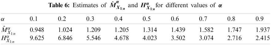
Based on this data, we used first the maximum likelihood method to estimate the exponential distribution parameter, λ^=0.122. Then, for different values of α, varied from 0.1 to 0.9, we calculate the estimated values of MX1:nα and HX1:nαof smallest order statistics under exponential distribution. The results are displayed in Tab. 6.

It should be noted that the estimated values of M^X1:nαis generally increased when 0<α<1. Also, the results in Tab. 6 indicate clearly that the estimated entropy values based on M^X1:nαare less than those given by HX1:nα.

The key focus of this article is to propose new quantile-based Mathai-Haubold entropy and investigate its characteristics. We also considered the divergence measure of the Mathai-Haubold and established some of its properties. Further, based on order statistics, we propose the residual entropy of the quantile-based Mathai-Haubold and some of its property results are proved. The performance of the proposed quantile-based Mathai-Haubold entropy is investigated by simulation studies and also by using real data application example. The proposed quantile-based Mathai-Haubold entropy's performance is investigated by simulation studies and by using a real data application example. We found that the ML estimates of MX1:nα approach true value when sample size n increases for the simulation part. For the application part, we compared our proposed quantile-based entropy to the existing quantile entropies and the results showed the outperformance of our proposed entropy to the other entropies. Our proposed quantile-based Mathai-Haubold entropy is useful for many future engineering applications such as reliability and mechanical components analysis.

Quantile functions are efficient and equivalent alternatives to distribution functions in modeling and analysis of statistical data. The scope of these functions and the probability distributions are essential in studying and analyzing real lifetime data. One reason is that they convey the same information about the distribution of the underlying random variable X. However, even if sufficient literature is available on probability distributions' characterizations employing different statistical measures, little works have been observed for modeling lifetime data using quantile versions of order statistics. Therefore, future work is necessary for enriching this area, and for this reason, we give precise recommendations for future research. First, the results obtained in this article are general because they can be reduced to some of the results for quantile based Shannon entropy for order statistics once parameter approaches unity. Recently, a quantile version of generalized entropy measure for order statistics for residual and past lifetimes was proposed by Kumar et al. [22]. Nisa et al. [23] presented a quantile version of two parametric generalized entropy of order statistics residual and past lifetimes and derived some characterization results. Moreover, Qiu [24] studied further results on quantile entropy in the past lifetime and gave the quantile entropy bounds in the past lifetime for some ageing classes. The ideas presented by these mentioned papers can be somehow combined/merged with our results in this paper to produce more results and properties for the quantile-based Mathai-Haubold. Second, Krishnan [25] recently introduced a quantile-based cumulative residual Tsallis entropy (CRTE) and extended the quantile-based CRTE in the context of order statistics. Based on these new results and our proposed quantile M-H entropy in this paper, one can follow Krishnan [25] and derive a quantile-based cumulative residual M-H entropy and extend it in the context of order statistics. Finally, Krishnan [25] also proposed a cumulative Tsallis entropy in a past lifetime based on quantile function. As an extension, the cumulative M-H entropy in a past lifetime based on quantile function can also be derived.

Acknowledgement: The authors would like to thank the anonymous reviewers and the editor for their useful suggestions and comments which increase and improve the quality of this paper.

Funding Statement: Authors thank and appreciate funding this work by the Deanship of Scientific Research at King Khalid University through the Research Groups Program under the Grant No. (R.G.P. 2/82/42).

Conflicts of Interest: The authors declare that they have no conflicts of interest to report regarding the present study.

References

Arnold, B. C., Blakrishan, N., Nagraja, N. H. (1992). A first course in order statistics. New York: John Wiley and Sons.
Malik, J. H., Balakrishnan, N., & Ahmad, S. E. (1998). Recurrence relations and identities for moments of order statistics I: Arbitrary continuous distributions. Communication in Statistics–Theory and Methods, 17(8), 2623-2655. [Google Scholar] [CrossRef]
Samuel, P., & Thomas, P. Y. (2000). An improved form of a recurrence relation on the product moment of order statistics. Communication in Statistics-Theory and Methods, 29(7), 1559-1564. [Google Scholar] [CrossRef]
David, H. A. (1981). Order statistics. Second Edition. New York: John Willey and Sons.
Shannon, C. E. (1948). A mathematical theory of communication. Bell System Technical Journal, 27, 379-423. [Google Scholar] [CrossRef]
Mathai, A., & Haubold, H. (2007). On generalized entropy measures and pathways. Physica A: Statistical Mechanics and its Applications, 385(2), 493-500. [Google Scholar] [CrossRef]
Sebastian, N. (2015). Generalized pathway entropy and its applications in diffiusion entropy analysis and fractional calculus. Communications in Applied and Industrial Mathematics, 6(2), 1-20. [Google Scholar] [CrossRef]
Mathai, A. (2005). A pathway to matrix-variate gamma and normal densities. Linear Algebra and its Applications, 396, 317-328. [Google Scholar] [CrossRef]
Nair, N. U., & Sankaran, P. G. (2009). Quantile-based reliability analysis. Communication in Statistics-Theory and Methods, 38, 222-232. [Google Scholar] [CrossRef]
Sunoj, S. M., Krishnan, A. S., & Sankaran, P. G. (2017). Quantile-based entropy of order statistics. Journal of the Indian Society for Probability and Statistics, 18(1), 1-17. [Google Scholar] [CrossRef]
Sunoj, S. M., & Sankaran, P. G. (2012). Quantile based entropy function. Statistics and Probability Letters, 82(6), 1049-1053. [Google Scholar] [CrossRef]
Wong, K. M., & Chen, S. (1990). The entropy of ordered sequences and order statistics. IEEE Transaction Information Theory, 36, 276-284. [Google Scholar] [CrossRef]
Park, S. (2007). The entropy of consecutive order statistics. IEEE Transaction Information Theory, 41(6), 2003-2007. [Google Scholar] [CrossRef]
Ebrahimi, N. (1996). How to measure uncertainty in the residual lifetime distribution. Sankhya SerA, 58, 48-56. [Google Scholar]
Baratpour, S., Ahmadi, J., & Arghami, N. R. (2007). Some characterizations based on entropy of order statistics and record values. Communications in Statistical-Theory and Methods, 36, 47-57. [Google Scholar] [CrossRef]
Paul, J., & Yageen, P. (2019). On some properties of Mathai-Haubold entropy of record values. Journal of the Indian Society for Probability and Statistics, 20(1), 31-49. [Google Scholar] [CrossRef]
Kullback, S., & Leibler, R. A. (1951). On information and sufficiency. Annals of Mathematical Statistics, 22, 79-86. [Google Scholar] [CrossRef]
Dar, J. G., & Al-Zahrani, B. (2013). On some characterization results of life time distributions using Mathai-Haubold residual entropy. International Organization of Scientific Research, 5(4), 56-60. [Google Scholar] [CrossRef]
Crescenzo, A. D., & Longobardi, M. (2002). Entropy based measure of uncertainty in past lifetime distribution. Journal of Applied probability, 39(2), 434-440. [Google Scholar] [CrossRef]
Murthy, D. N. P., Xie, M., Jiang, R. Y. (2004). Weibull models. USA: John Wiley & Sons.
Kumar, V. R. (2018). A quantile approach of Tsallis entropy for order statistics. Physica A: Statistical Mechanics and its Applications, 503, 916-928. [Google Scholar] [CrossRef]
Kumar, V., & Singh, N. (2019). Quantile-based generalized entropy of order (α, β) for order statistics. Statistica, 78(4), 299-318. [Google Scholar] [CrossRef]
Nisa, R., & Baig, M. A. K. (2019). Characterization results based on quantile version of two parametric generalized entropy of order statistics. Journal of Probability and Mathematical Statistics, 1, 1-17. [Google Scholar] [CrossRef]
Qiu, G. (2019). Further results on quantile entropy in the past lifetime. Probability in the Engineering and Informational Sciences, 33(1), 149-159. [Google Scholar] [CrossRef]
Krishnan, A. S. (2019). A study on some information measures using quantile functions (Ph.D. Thesis). Cochin University of Science and Technology, India.