| Computer Modeling in Engineering & Sciences |
DOI: 10.32604/cmes.2021.016894
ARTICLE
Functionally Graded Cellular Structure Design Using the Subdomain Level Set Method with Local Volume Constraints
1Department of Engineering Mechanics, School of Civil Engineering, Wuhan University, Wuhan, 430072, China
2State Key Laboratory for Structural Analysis of Industrial Equipment, Dalian University of Technology, Dalian, 116024, China
3School of Mechanics and Engineering, Southwest Jiaotong University, Chengdu, 611756, China
*Corresponding Author: Hui Liu. Email: h.liu@whu.edu.cn
Received: 7 April 2021; Accepted: 24 May 2021
Abstract: Functional graded cellular structure (FGCS) usually shows superior mechanical behavior with low density and high stiffness. With the development of additive manufacturing, functional graded cellular structure gains its popularity in industries. In this paper, a novel approach for designing functionally graded cellular structure is proposed based on a subdomain parameterized level set method (PLSM) under local volume constraints (LVC). In this method, a subdomain level set function is defined, parameterized and updated on each subdomain independently making the proposed approach much faster and more cost-effective. Additionally, the microstructures on arbitrary two adjacent subdomains can be connected perfectly without any additional constraint. Furthermore, the local volume constraint for each subdomain is applied by virtue of the augmented Lagrange multiplier method. Finally, several numerical examples are given to verify the correctness and effectiveness of the proposed approach in designing the functionally graded cellular structure. From the optimized results, it is also found that the number of local volume constraints has little influence on the convergence speed of the developed approach.
Keywords: Multiscale design; hierarchical structure; functionally graded cellular structure; local volume constraints; topology optimization
Functionally graded cellular structure (FGCS), composed of an interconnected network of bars or plates, is usually designed to attain a specific purpose. With low density and high stiffness and strength [1], FGCS shows superior performance than traditional structure [2,3]. The cellular structure leads to good thermal diffusion efficiency, strong energy absorption effect and shocking resistance. Another advantage of FGCS is that it usually keeps working properly when some local failures or defects occur. That’s to say, FGCS is not sensitive to local defects. Consequently, FGCS is widely used in the aerospace, medical and other industries [4,5].
The geometric configuration of the microstructures making up the cellular structure can be regular or irregular. The honeycomb and the lattice structures belong to the former, while the foam is the latter. The cellular structure has been studied intensively in the last few decades. Analytical and experimental investigations were conducted to derive the detailed expression of the effective thermal conductivity, permeability and the inertial coefficient of metal foams [6–10]. It showed that the lattice structure has an inherent advantage over foams in resisting shock waves and bending due to its periodic characteristics [11,12]. Of course, cell pattern has a significant influence on failure mode and energy absorption [13,14]. The honeycomb structures was introduced at length in [15] with its application and tests.
Nowadays, with the development of additive manufacturing (AM), the field of structure manufacturing has been ushered into an era of rapid development, which expands the application prospect of topology optimization at the same time. Topology optimization techniques are gradually being used for the design of AM parts and are in focus in the ongoing research of AM community [16]. Using additive manufacturing technology, people can realize the manufacture of FGCS [17,18]. New computer aided design methods are developed for AM to deal with the complex geometry of cellular structures. Aremu et al. [19] gained insight into the performance of two variants of AM lattice and demonstrated the great potential of AM technology. A number of approaches were developed to design the FGCS, such as relative density mapping method [20], the size and scaling method [21], and the isostatic lines approach [22].
Topology optimization turns out to be powerful in realizing structural design. Over the last few decades, a variety of optimization methods have been developed [23–26]. Recently, more and more topological optimization-based algorithms are proposed to design cellular structure, such as the projection or mapping methods [27,28], the scale related-based two scales methods [29–34]. In the current research status, the connectivity between adjacent microstructures has become an important problem to be solved. Song et al. [35] designed a kind of irregular cellular structure based on a modified Solid Isotropic Material with Penalization (SIMP) method and validated its superiority through experiment. Radman et al. [36] used the Bi-directional Evolutionary Structure Optimization (BESO) method to design cellular functionally graded materials via variation in stiffness along a certain direction. Zhang et al. [37] developed the design element concept to design the cellular structures by considering the materials and structures in a unified way. Li et al. [38] developed a multi-scale topology optimization method for the integrated design of functional graded cellular composites. Wang et al. [39] presented a concurrent design method based on micro-architectures. Li et al. [40] developed a density-based topology optimization method for cellular structures with quasi-periodic microstructures by employing the erode-dilate operators. Zhu et al. [41] established an efficient method to design the infilled graded structures based on the asymptotic homogenization theory. We proposed a new subdomain parameterized level set method [42] which is much more cost-effective compared to the classical method since the parameterization process can be achieved in parallel on each subdomain. Zong et al. [43] presented a variable cutting level set method to design FGCS. By introducing a variable and continuous cutting function, it can guarantee perfect geometric connections between adjacent cells. Further, Liu et al. [44] developed a multiple variable cutting (M-VCUT) level set method for designing the cellular structures. As a generalization of the VCUT level set method, connections between microstructures in neighboring cells are naturally guaranteed without any extra constraints.
There is a great demand for functionally graded cellular structure in practical engineering. Usually, the geometric complexity of the structures obtained by considering local volume constraints (LVC) are significantly higher than those obtained by considering global volume constraints. The structures with higher geometric complexity sometimes meet the need of engineering better, such as load bearing, impact resistance and anti-disturbance caused by defects. Cai et al. [45] investigated the volume constraints on the subdomain of a continuum structure topology optimization using a heuristic approach. Hesse et al. [46] considered multiple, arbitrarily placed, volume constraints in shape topology based on the level-set optimization framework. Wu et al. [47] raised a method to generate bone-like porous structures by putting LVC in the design domain.
In this paper, we propose a strategy to generate FGCS utilizing the subdomain parameterized level set method with local volume constraints, where the material volume usage for each subdomain could be restricted in a uniform or non-uniform form. By parameterizing and updating the level set function on each subdomain, the subdomain parameterized level set method is more efficient than the classical parameterized level set method since the parameterization process could be proceeded only on each subdomain independently and efficiently. In addition, arbitrary adjacent two microstructures can be connected perfectly and automatically by using the subdomain level set method since the sensitivity analysis is conducted on the whole (global) design domain. By introducing the local volume constraints into the subdomain level set method, the FGCS can be easily obtained. Furthermore, an easy-to-implement regularization method is employed in this paper to solve the mesh-dependency problem of the optimized results.
This paper is organized as follows. Firstly, the subdomain parameterized level set method with local volume constraints (LVC) is described in detail in the next section. Then, to verify the correctness and effectiveness of the developed approach, some numerical examples are conducted in Section 3. Finally, conclusions are drawn in Section 4.
2 The Subdomain Parameterized Level Set Method with Local Volume Constraints
2.1 The Classic Level Set Method
Osher et al. [48] firstly raised the level set method to tackle fronts propagating with curvature-dependent speed. Sethian et al. [49] and Osher et al. [50] applied the approach to the structure optimization. Allaire et al. [51] and Wang et al. [24] put forward the level set method with the shape derivative for structural topology optimization. Compared with the element based topology optimization algorithms, such as the SIMP and the BESO, the level set based topology optimization method can generate structural configuration with smooth and clear boundaries.
As shown in Fig. 1, in the level set method, the zero isosurface of a higher dimensional level set function
where
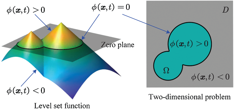
Figure 1: Representing a two dimensional problem with a level set function
In the classical level set method, a signed distance function is usually used as the level set function. Through the evolution of the level set function, the structural boundary can be changed implicitly. In the classical level set method, the level set function
where
During the solving of the above-mentioned Hamilton-Jacobi equation, some issues may be caused: (a) the level set function must be re-initialized frequently to maintain a signed distance function, which is important to keep the normal gradient of the level set function constant; (b) the time step is required to be small enough and satisfy the Courant-Friedrichs-Lewy (CFL) condition to ensure the numerical stability; (c) new holes are difficult to be created inside the solid material domain.
2.2 The Subdomain Parameterized Level Set Method
To overcome the above-mentioned issues, Wang et al. [52] proposed a parametric level set method for shape and topology optimization using radial basis functions (RBFs). Wei et al. [53] presented a compact and efficient code based on the parameterized level set method. Recently, we proposed a subdomain parameterized level set method [42] for designing the cellular structures. In this approach, the whole design domain D and structural domain
where M is the number of subdomains within the whole design domain, M = 2 for the subdomain division in Fig. 2a. On each subdomain, a subdomain level set function
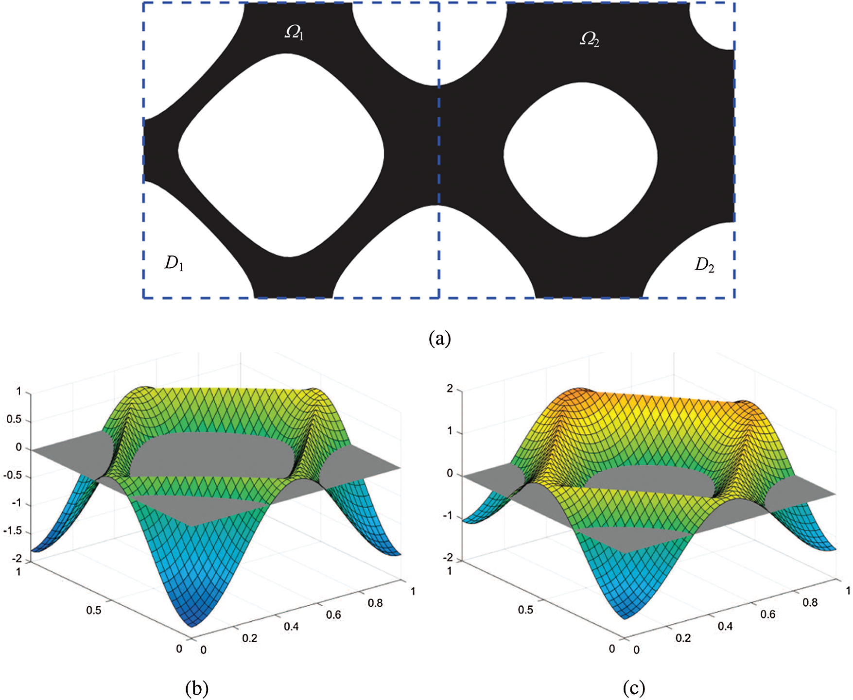
Figure 2: A design domain divided into two subdomains: (a) subdomain division; (b) subdomain level set function
Then, a subdomain level set function
Then the evolution of
where
The above-mentioned issues encountered in solving the HJ equation can be overcome by parameterizing the level set function with any spatial discretization approach. In this work, the radial basis functions (RBFs) is introduced for parameterizing the subdomain level set function
where
The subdomain level set function
where Ns is the number of knots of the RBFs on the subdomain Ds,
To ensure the uniqueness of the solution, the following orthogonal conditions [53,54] should be met:
By substituting the coordinates
where
Substituting Eq. (10) into Eq. (5), the following HJ equation in a matrix-vector form can be obtained:
where
in which
By parameterizing the level set function with the RBFs, the evolution of
where
2.3 Sensitivity Analysis of the Objective Function and the Constraints
The compliance problem of the optimized structure is considered in the work. According to the level set method, the mathematical formulation is given as
where
The normal velocity field of the boundaries of the whole structures
where
The normal velocity field
where
where
In the first NR iteration, the volume constraint is relaxed as
where
2.4 Meshes in the Optimization
In general, in the subdomain level set method, the mesh for discretizing the microstructure and the one for parameterizing the subdomain level set function on each subdomain could be different. However, for the convenience of calculation, these two sets of meshes are set to the same, i.e., the knots of the RBFs are the same to the nodes of the finite element mesh on each subdomain.
As shown in Fig. 3, the full-scale mesh generated on the whole design domain D is used for obtaining the displacement field (u, v) and the global normal velocity field
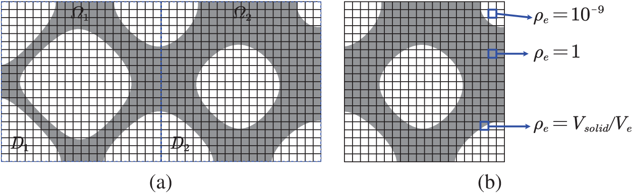
Figure 3: Meshes used in the subdomain level set method: (a) full-scale mesh for the whole design domain D; (b) sub grids for the subdomain D2
A stiffness reduction factor
where De means the design domain of element;
As a result, the stiffness matrix of an element can be expressed as
In order to eliminate mesh dependency during the topology optimization, a simple filtering approach [55,56] is employed in this paper to obtain mesh independent optimized results. The filter is defined as
where Ni is the set of nodes j for which the node-to-node distance
A cantilever beam model is taken into account herein to verify the effectiveness of the filtering approach. The design domain, boundary conditions and initial material distribution of the cantilever beam model are shown in Fig. 4, where W = 1 and F = 1. The Young’s modulus and Poisson’s ratio are E = 1 and
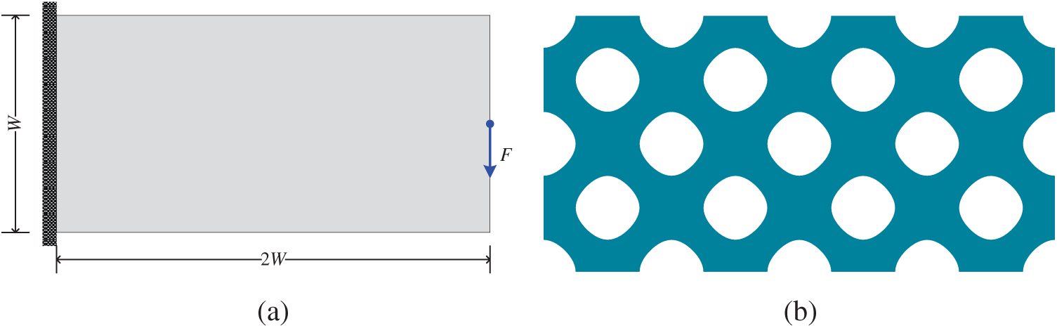
Figure 4: Cantilever model and its initial design. (a) cantilever beam model (b) initial design
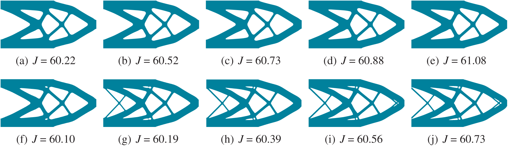
Figure 5: Comparison of the optimized results: (a)
2.6 The Local Volume Constraints
In the structural topology optimization, global material volume constraints are usually used. Under global material volume constraints, large area of the optimized structures have no material or solid material, as illustrated in Fig. 5.
As mentioned in the introduction part, the functionally graded cellular structures could be designed by virtue of the local volume constraints [45,47]. In this work, the local volume constraints are applied for generating the FGCS based on our previous developed subdomain level set method [42].
For the local volume constrains, the upper limit of material usgae is different in different positions. Generally, one should set the upper limit of material usage a little higher at the location with larger stress, strain or strain energy, while it should be set lower at the location with smaller stress. In this paper, the coarse-scale mesh and the subdomain division are the same, i.e., a coarse-scale element corresponds to a subdomain. There are two ways to provide the local volume constraints for all the subdomains. The first way is to use the SIMP method on the coarse-scale mesh (subdomain division) without density penalization, i.e., p = 1, to generate a gray structure, where the virtual density is regarded as the upper limit of the material volume fraction the volume fraction which is used as a constraint in the proposed subdomain level set method. The second is to manually specify the material volume constraints for each subdomain. The calculation process of the proposed method is given as follows:
1. initialize
2. k = 1, while k < kmax, do
3. obtain
4. obtain filtered level set function
5. solve static equilibrium equation of the structure;
6. calculate
7. obtain
8. update the coefficients of the RBFs by Eq. (17);
9. update the level set function
10. check convergence;
11. if convergence, break the while loop; if not, k = k + 1, then go to Step 3;
12. end while
13. obtain
In this section, several examples are carried out to show the effectiveness of the proposed algorithm. It should be mentioned that the initial design of microstructure defined on each subdomain is shown in Fig. 6.

Figure 6: Initial design defined on each subdomain: (a) initial microstructure; (b) the subdoman level set function corresponding to the initial microstructure
3.1 Predefined Local Volume Constraints
Four examples are carried out in this subsection to verify the effectiveness and correctness of the proposed subdomain parameterized level set method with local volume constraints. The first one is a cantilever beam model as shown in Fig. 7a with the left edge fixed and a unit concentrated force applied on middle point of the right edge along the negative vertical direction. The second one is a simply supported beam model as shown in Fig. 8a with a concentrated force imposed on the middle of the upper beam. The third and the fourth ones are the computational models with multiple load cases, the former is a cantilever beam model shown in Fig. 9a with the left edge fixed and a unit concentrated force applied on the bottom right corner and the upper right corner while the latter is a simply supported beam model shown in Fig. 10a subjected to three forces respectively at 1/4, 1/2 and 3/4 of the upper edge. The Young’s modulus, the Poisson’s ratio and the thickness of the model are set as E = 1,
By using the SIMP method without penalization (p = 1), several gradient variable density planar structures can be obtained easily, as shown in Figs. 7b, 8b, 9b and 10b, respectively. In these figures, the density on each coarse-scale element can be seen as the volume fraction constraint of the material usage on each corresponding subdomain in the calculation of the proposed subdomain level set method with local volume constraints, i.e.,
where
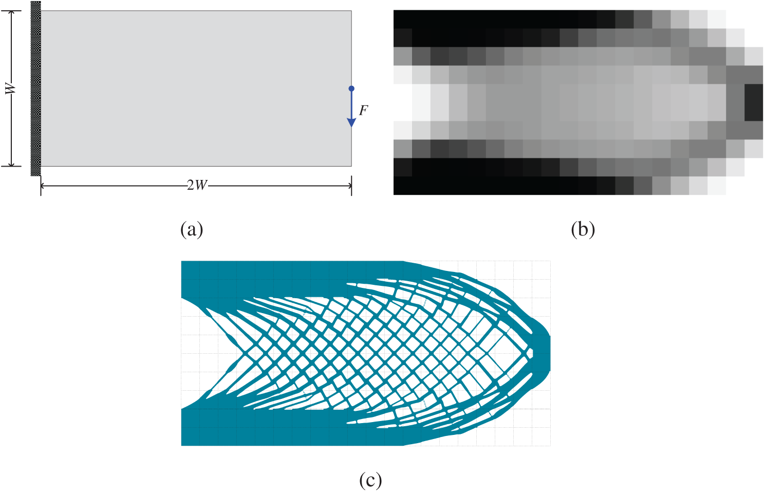
Figure 7: Optimization of a cantilever beam model: (a) design domain and its boundary conditions; (b) coarse-scale design obtained by using the SIMP method with p = 1; (c) optimized cellular structure by using the proposed subdomain level set method with local volume constraints

Figure 8: Optimization of a simple supported beam model: (a) design domain and its boundary conditions; (b) coarse-scale design obtained by using the SIMP method with p = 1; (c) optimized cellular structure by using the proposed subdomain level set method with local volume constraints
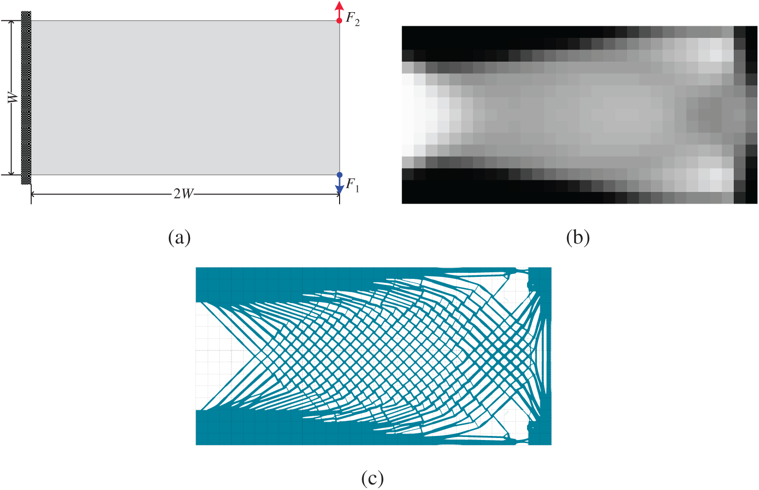
Figure 9: Optimization of a cantilever model under two load cases: (a) design domain and its boundary conditions; (b) coarse-scale design obtained by using the SIMP method with p = 1; (c) optimized cellular structure by using the proposed subdomain level set method with local volume constraints
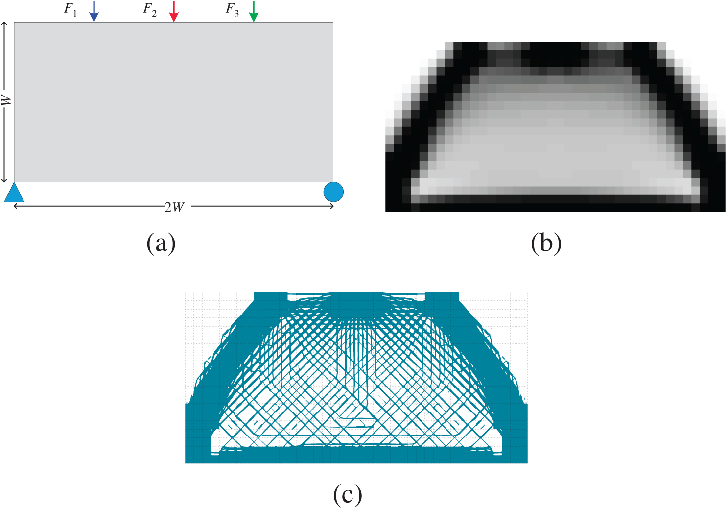
Figure 10: Optimization of a model under three load cases: (a) design domain and its boundary conditions; (b) coarse-scale design obtained by using the SIMP method with p = 1; (c) optimized cellular structure by using the proposed subdomain level set method with local volume constraints
Based on these local volume constraints, four different optimized cellular structures as shown in Figs. 7c, 8c, 9c, and 10c, respectively. By using the proposed subdomain level set method with local volume constraints, the gradient cellular structures with clear boundaries can be easily obtained. By comparing these two optimization results, we can see that the material volume distributions are macroscopically the same, which indicates that the imposed local volume constraints are satisfied. For the black area of the coarse-scale design results (the coarse elements with the density being equal to 1), the counterpart subdomains are filled with solid material. For the white areas, the counterpart subdomains are filled void material. For the gray areas, gradient cellular structures are filled in the counterpart subdomains. In addition, the microstructures of adjacent subdomains have good connectivity on their common boundaries. In a word, the subdomain parameterized level set method can get a clear structure boundary making the structure easy to be manufactured. If the material usage requirements for all subdomains can be estimated in advance in the process of structural topology optimization, the method proposed in this paper can realize the design of the cellular structure based on the predefined local volume constraints.
The convergence histories of these four examples are shown in Fig. 11, where the compliances fall fast in the beginning 20 steps approximately and reaches a minimize value. After that, it gradually rises to the local maximum value, then slowly declines and finally tends to a stable value. Based on the calculation results, we can find that no matter what the structure is and how many the subdomains are, the optimizations converge after about 150 steps. This indicates that the number of local volume constraints has little influence on the convergence speed of the algorithm of the presented method.
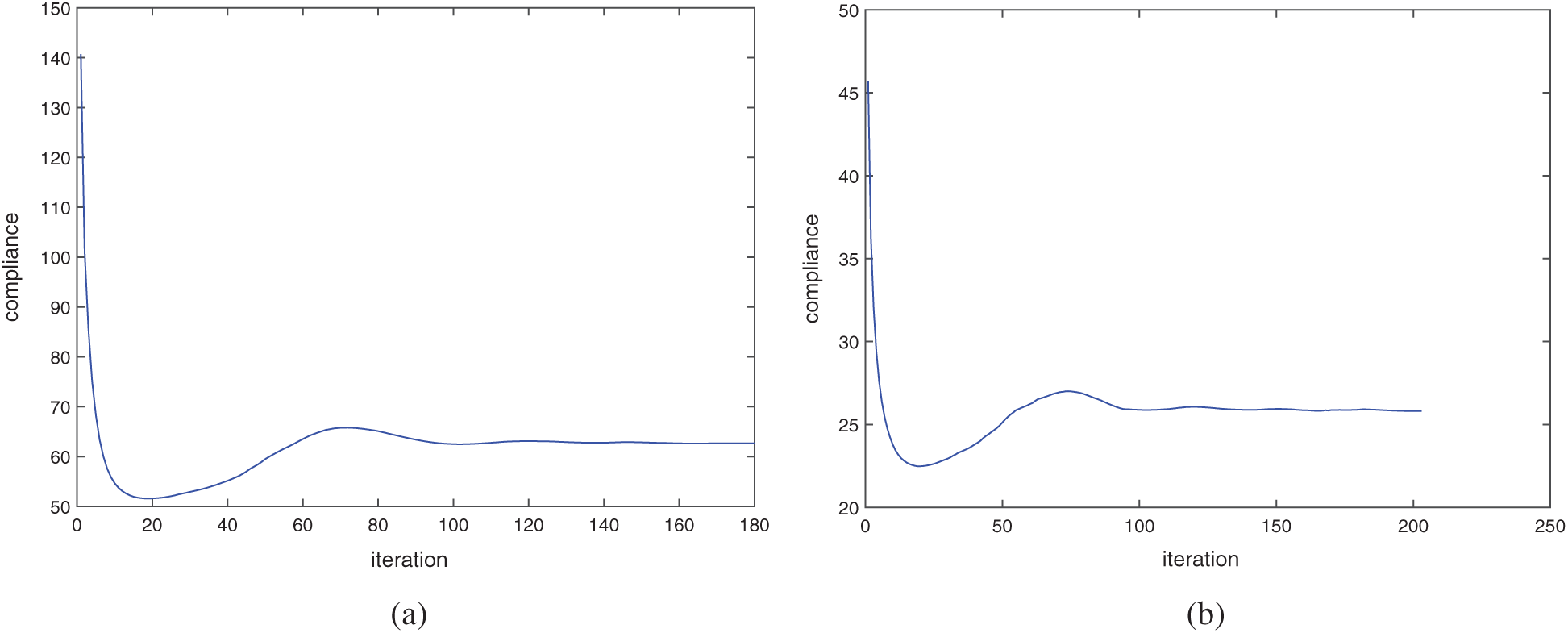
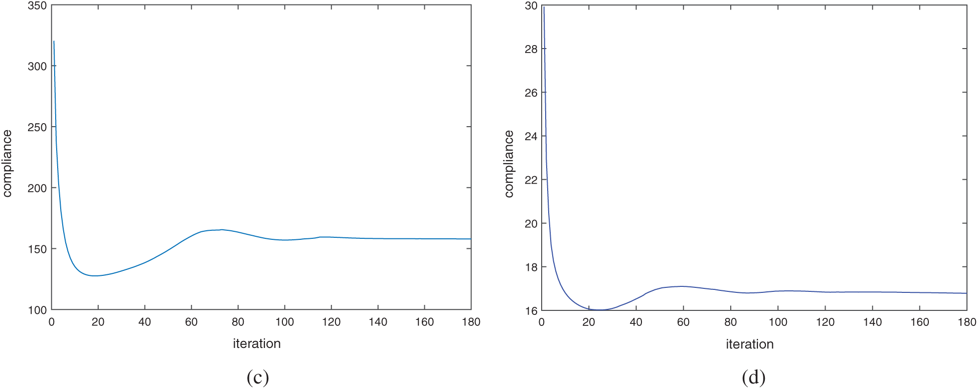
Figure 11: Iteration history of objective function: (a) the cantilever beam model as shown in Fig. 7; (b) the model as shown in Fig. 8; (c) the cantilever beam model under two load cases as shown in Fig. 9; (d) the model under three load cases as shown in Fig. 10
3.2 Gradient Cellular Structural Design
Three cases in this subsection are conducted to illustrate the effectiveness of the presented subdomain level set method with local volume constraints when designing the functionally graded cellular structure. All the cases are carried out based on the cantilever beam model shown in Fig. 12a. Their coarse-scale meshes for the cases are the same as shown in Fig. 12b, where the whole design domain is divided into
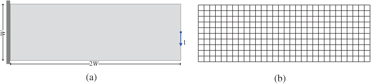
Figure 12: Cantilever beam model: (a) design domain and boundary conditions; (b) coarse-scale mesh/subdomain division

Figure 13: Volume fraction upper limit of each subdomain and the corresponding optimized results: (a) uniform volume fraction upper limits; (b) optimized cellular structure based on the uniform local volume constraints shown in (a); (c) Monotonically decreasing volume fraction upper limits; (d) optimized cellular structure based on the local volume constraints shown in (c); (e) Fluctuating volume fraction upper limits; (f) optimized cellular structure based on the local volume constraints shown in (e)
Three different distributions of the volume fraction upper limit for each subdomain are shown in Figs. 13a, 13c, and 13e, respectively, which represent three different local volume constraints, i.e., uniform distributed LVC, monotonically decreasing distributed LVC, and fluctuating distributed LVC. Based on these three different local volume constraints, the optimized gradient cellular structures are obtained by using the proposed subdomain level set method and they are presented in Figs. 13b, 13d, and 13f, respectively. As shown in Fig. 13b, the material distribution at the upper and lower ends of the structure is rather concentrated, which is mainly used to bear the bending moment. The intermediate material distribution is relatively uniform, showing the cellular distribution. The optimized structures in Fig. 13 are similar to each other basically, but there is a little difference to be pointed out. It can be seen from Fig. 13d that the structure presents gradient change from the left to right duo to the graded local volume constraints. The material distribution on the left parts of the structure is denser and then becomes sparse from the left to right. While the material distribution in Fig. 13f presents a dense-sparse alternation pattern. The compliances of these optimized structures are 235.75, 209.63 and 245.95 for the above-mentioned three local volume constraints, respectively. The structure obtained by local volume constraints which are monotonically decreasing from the left to right is stiffer than the other two cases. From the optimization results, each subdomain can meet the specified volume constraints. This further validates the correctness and effectiveness of the proposed method.
Another advantage of cellular structure is that it is not sensitive to local defects. When local damage occurs, the cellular structure still maintains a nice integrity. In practical, many factors will lead to local failure, such as local stress concentration, damage fatigue, manufacturing error and other accidental events. They usually decide the kind of cracks and holes of different shapes and sizes in material failure. For convenience, we introduce a simplified model of material removal to tackle the complicated problem in the optimization process [57]. In other word, the volume fraction of the subdomain to be removed is changed into zero. Theoretically, when an optimized structure suffers from local failure, the stiffness of the structure will be reduced significantly. Consequently, the structure may no longer bear any loads or even be destroyed. If a structure can still maintain good stiffness when the local damage happens, it indicates that the structure is rather stable and not sensitive to local defects.
Three cantilever beams examples, whose computational model and boundary conditions are the same as the cantilever model shown in Fig. 7a, are carried out for comparison to illustrate the defect sensitivity of cellular structure. The results in the first row of Fig. 14 are obtained by using the SIMP method on the coarse-scale mesh of
Figure 14: Effects of defects (marked in yellow) on structural performance (objective function): (a) and (b) structures optimized by using the SIMP method with p = 3 based on the coarse-scale mesh; (c) and (d) structures optimized by using the subdomain level set method based on the fine-scale mesh; (e) and (f) structures optimized by using the SIMP method with p = 3 based on the fine-scale mesh
The compliance values of the structures before and after considering local defects are shown in Fig. 14, where Jo and Jd denote the compliance values of structures without and with considering local defect, respectively. We can see that the compliance of the structure in Figs. 14a and 14b is Jo = 91.39 when the structure is in good condition while increased to Jd = 200.25 and Jd = 1000.04 when two different defects occur. While the compliance of the optimized cellular structure in Figs. 14c and 14d is only increased from Jo = 62.64 to Jd = 71.12 and Jd = 65.79 when the two defects occur. The compliance of the optimized structure by using the SIMP method with the filter radius rmin = 1.2 le on the fine-scale mesh in Figs. 14e and 14f, where le denotes the size of element, is changed from Jo = 61.23 to Jd = 159.76 and Jd = 82.43 when the defects occur. For the traditional optimized structures by using the SIMP method with penalization, by comparison with the compliance of the structure without considering defect, the compliance of the structure obtained based on the coarse-scale mesh increased by
A subdomain level set based topology optimization method is developed for designing the functionally graded cellular structure by imposing the local volume constraint on each subdomain. The microstructures on adjacent subdomains can be connected automatically by using the proposed method. A simple filtering approach is employed into the proposed subdomain level set method for generating mesh independent results. Two ways are provided in this paper to generate the material volume constraints for all the subdomains. The first is to use the SIMP method on the coarse-scale mesh without p = 1 to generate local volume fraction upper limit for each subdomain. The second is to manually specify the material volume constraints for each subdomain. By using the predefined local volume constrains, we can obtain gradient cellular structures with the developed method. Several numerical examples are carried out for verifying the effectiveness and correctness of the presented method. Computation results show that the number of local volume constraints has little influence on the convergence speed of the proposed method. By comparison with the traditional structure optimized by using the SIMP method with density penalization, i.e., p = 3, it is found that the gradient cellular structure optimized by using the proposed method is less sensitive to local defect.
Acknowledgement: The authors wish to express their appreciation to the reviewers for their helpful suggestions which greatly improved the presentation of this paper.
Funding Statement: This work is supported by the National Natural Science Foundation of China (Grant Nos. 12072242, 11772237), the Natural Science Foundation of Hubei Province (Grant No. 2020CFB816) and the open funds of the State Key Laboratory of Structural Analysis for Industrial Equipment (Dalian University of Technology) through contract/Grant No. GZ19110.
Conflicts of Interest: The authors declare that they have no conflicts of interest to report regarding the present study.
1. Penzien, J., Didriksson, T. (1964). Effective shear modulus of honeycomb cellular structure. AIAA Journal, 2(3), 531–535. DOI 10.2514/3.2346. [Google Scholar] [CrossRef]
2. Schaedler, T. A., Carter, W. B. (2016). Architected cellular materials. Annual Review of Materials Research, 46(1), 187–210. DOI 10.1146/annurev-matsci-070115-031624. [Google Scholar] [CrossRef]
3. Gibson, L. J. (1989). Modelling the mechanical behavior of cellular materials. Materials Science and Engineering A, 110(2), 1–36. DOI 10.1016/0921-5093(89)90154-8. [Google Scholar] [CrossRef]
4. Nguyen, J., Park, S. I., Rosen, D. (2013). Heuristic optimization method for cellular structure design of light weight components. International Journal of Precision Engineering and Manufacturing, 14(6), 1071–1078. DOI 10.1007/s12541-013-0144-5. [Google Scholar] [CrossRef]
5. Li, D., Liao, W., Dai, N., Dong, G., Tang, Y. et al. (2018). Optimal design and modeling of gyroid-based functionally graded cellular structures for additive manufacturing. Computer-Aided Design, 104(2), 87–99. DOI 10.1016/j.cad.2018.06.003. [Google Scholar] [CrossRef]
6. Ashby, M. F., Evans, A. G., Fleck, N. A., Gibson, L. J., Hutchinson, J. W. et al. (2012). Metal foams: A design guide. Butterworth-Heinemann. DOI 10.1016/B978-0-7506-7219-1.X5000-4. [Google Scholar] [CrossRef]
7. Boomsma, K., Poulikakos, D. (2001). On the effective thermal conductivity of a three-dimensionally structured fluid-saturated metal foam. International Journal of Heat and Mass Transfer, 44(4), 827–836. DOI 10.1016/S0017-9310(00)00123-X. [Google Scholar] [CrossRef]
8. Bhattacharya, A., Calmidi, V. V., Mahajan, R. L. (2002). Thermophysical properties of high porosity metal foams. International Journal of Heat and Mass Transfer, 45(5), 1017–1031. DOI 10.1016/S0017-9310(01)00220-4. [Google Scholar] [CrossRef]
9. Banhart, J. (2001). Manufacture, characterisation and application of cellular metals and metal foams. Progress in Materials Science, 46(6), 559–632. DOI 10.1016/S0079-6425(00)00002-5. [Google Scholar] [CrossRef]
10. Evans, A. G., Hutchinson, J. W., Fleck, N. A., Ashby, M. F., Wadley, H. N. G. (2001). The topological design of multifunctionally cellular metals. Progress in Materials Science, 46(3), 309–327. DOI 10.1016/S0079-6425(00)00016-5. [Google Scholar] [CrossRef]
11. Rashed, M. G., Ashraf, M., Mines, R. A. W., Hazell, P. J. (2016). Metallic microlattice materials: A current state of the art on manufacturing, mechanical properties and applications. Materials & Design, 518–533. DOI 10.1016/j.matdes.2016.01.146. [Google Scholar] [CrossRef]
12. Wadley, H. N. G. (2006). Multifunctionally periodic cellular metals. Philosophical Transactions of the Royal Society London, Series A, 364(1838), 31–68. DOI 10.1098/rsta.2005.1697. [Google Scholar] [CrossRef]
13. Ajdari, A., Nayebhashemi, H., Vaziri, A. (2011). Dynamic crushing and energy absorption of regular, irregular and functionally graded cellular structures. International Journal of Solids and Structures, 48(3–4), 506–516. DOI 10.1016/j.ijsolstr.2010.10.018. [Google Scholar] [CrossRef]
14. Wadley, H. N. G., Fleck, N. A., Evans, A. G. (2003). Fabrication and structural performance of periodic cellular metal sandwich structures. Composites Science and Technology, 63(16), 2331–2343. DOI 10.1016/S0266-3538(03)00266-5. [Google Scholar] [CrossRef]
15. Zhang, Q., Yang, X., Li, P., Huang, G., Feng, S. et al. (2015). Bioinspired engineering of honeycomb structure-using nature to inspire human innovation. Progress in Materials Science, 74, 332–400. DOI 10.1016/j.pmatsci.2015.05.001. [Google Scholar] [CrossRef]
16. Panesar, A., Abdi, M., Hickman, D., Ashcroft, I. (2018). Strategies for functionally graded lattice structures derived using topology optimization for additive manufacturing. Additive Manufacturing, 19(2121), 81–94. DOI 10.1016/j.addma.2017.11.008. [Google Scholar] [CrossRef]
17. Cheng, L., Zhang, P., Biyikli, E., Bai, J., Robbins, J. et al. (2017). Efficient design optimization of variable-density cellular structures for additive manufacturing: Theory and experimental validation. Rapid Prototyping Journal, 23(4), 660–677. DOI 10.1108/RPJ-04-2016-0069. [Google Scholar] [CrossRef]
18. Chu, C., Graf, G., Rosen, D. W. (2008). Design for additive manufacturing of cellular structures. Computer-aided Design and Applications, 5(5), 686–696. DOI 10.3722/cadaps.2008.686-696. [Google Scholar] [CrossRef]
19. Maskery, I., Hussey, A., Panesar, A., Aremu, A., Tuck, C. et al. (2016). An investigation into reinforced and functionally graded lattice structures. Journal of Cellular Plastics, 53(2), 151–165. DOI 10.1177/0021955X16639035. [Google Scholar] [CrossRef]
20. Alzahrani, M., Choi, S., Rosen, D. W. (2015). Design of truss-like cellular structures using relative density mapping method. Materials & Design, 85(6), 349–360. DOI 10.1016/j.matdes.2015.06.180. [Google Scholar] [CrossRef]
21. Chang, P., Rosen, D. W. (2013). The size matching and scaling method: A synthesis method for the design of mesoscale cellular structures. International Journal of Computer Integrated Manufacturing, 26(10), 907–927. DOI 10.1080/0951192X.2011.650880. [Google Scholar] [CrossRef]
22. Daynes, S., Feih, S., Lu, W. F., Wei, J. (2017). Optimization of functionally graded lattice structures using isostatic lines. Materials & Design, 127(2121), 215–223. DOI 10.1016/j.matdes.2017.04.082. [Google Scholar] [CrossRef]
23. Sigmund, O. (2001). A 99 line topology optimization code written in matlab. Structural and Multidisciplinary Optimization, 21(2), 120–127. DOI 10.1007/s001580050176. [Google Scholar] [CrossRef]
24. Wang, M. Y., Wang, X., Guo, D. (2003). A level set method for structural topology optimization. Computer Methods in Applied Mechanics and Engineering, 192(1), 227–246. DOI 10.1016/S0045-7825(02)00559-5. [Google Scholar] [CrossRef]
25. Xie, Y. M., Steven, G. P. (1993). A simple evolutionary procedure for structural optimization. Computers & Structures, 49(5), 885–896. DOI 10.1016/0045-7949(93)90035-C. [Google Scholar] [CrossRef]
26. Guo, X., Zhang, W., Zhong, W. (2014). Doing topology optimization explicitly and geometrically–-A new moving morphable components based framework. Journal of Applied Mechanics, 81(8), 81009. DOI 10.1115/1.4027609. [Google Scholar] [CrossRef]
27. Groen, J. P., Sigmund, O. (2018). Homogenization-based topology optimization for high-resolution manufacturable microstructures. International Journal for Numerical Methods in Engineering, 113(8), 1148–1163. DOI 10.1002/nme.5575. [Google Scholar] [CrossRef]
28. Chen, W., Tong, L., Liu, S. (2017). Concurrent topology design of structure and material using a two-scale topology optimization. Computers & Structures, 178, 119–128. DOI 10.1016/j.compstruc.2016.10.013. [Google Scholar] [CrossRef]
29. Da, D., Cui, X., Long, K., Li, G. Y. (2017). Concurrent topological design of composite structures and the underlying multi-phase materials. Computers & Structures, 179(1), 1–14. DOI 10.1016/j.compstruc.2016.10.006. [Google Scholar] [CrossRef]
30. Kato, J., Yachi, D., Kyoya, T., Terada, K. (2018). Micro-macro concurrent topology optimization for nonlinear solids with a decoupling multiscale analysis. International Journal for Numerical Methods in Engineering, 113(8), 1189–1213. DOI 10.1002/nme.5571. [Google Scholar] [CrossRef]
31. Sivapuram, R., Dunning, P. D., Kim, H. A. (2016). Simultaneous material and structural optimization by multiscale topology optimization. Structural and Multidisciplinary Optimization, 54(5), 1267–1281. DOI 10.1007/s00158-016-1519-x. [Google Scholar] [CrossRef]
32. Vicente, W. M., Zuo, Z. H., Pavanello, R., Calixto, T. K. L., Picelli, R. et al. (2016). Concurrent topology optimization for minimizing frequency responses of two-level hierarchical structures. Computer Methods in Applied Mechanics and Engineering, 301(2), 116–136. DOI 10.1016/j.cma.2015.12.012. [Google Scholar] [CrossRef]
33. Alexandersen, J., Lazarov, B. S. (2015). Tailoring macroscale response of mechanical and heat transfer systems by topology optimization of microstructural details. Engineering and Applied Science Optimization, 38, 267–288. DOI 10.1007/978-3-319-18320-6. [Google Scholar] [CrossRef]
34. Xia, L., Breitkopf, P. (2015). Multiscale structural topology optimization with an approximate constitutive model for local material microstructure. Computer Methods in Applied Mechanics and Engineering, 286(6), 147–167. DOI 10.1016/j.cma.2014.12.018. [Google Scholar] [CrossRef]
35. Song, G., Jing, S., Zhao, F., Wang, Y., Xing, H. et al. (2017). Design optimization of irregular cellular structure for additive manufacturing. Chinese Journal of Mechanical Engineering, 30(5), 1184–1192. DOI 10.1007/s10033-017-0168-3. [Google Scholar] [CrossRef]
36. Radman, A., Huang, X., Xie, Y. M. (2013). Topology optimization of functionally graded cellular materials. Journal of Materials Science, 48(4), 1503–1510. DOI 10.1007/s10853-012-6905-1. [Google Scholar] [CrossRef]
37. Zhang, W., Sun, S. (2006). Scale-related topology optimization of cellular materials and structures. International Journal for Numerical Methods in Engineering, 68(9), 993–1011. DOI 10.1002/nme.1743. [Google Scholar] [CrossRef]
38. Li, H., Luo, Z., Zhang, N., Gao, L., Brown, T. (2016). Integrated design of cellular composites using a level-set topology optimization method. Computer Methods in Applied Mechanics and Engineering, 309(22–23), 453–475. DOI 10.1016/j.cma.2016.06.012. [Google Scholar] [CrossRef]
39. Wang, Y., Chen, F., Wang, M. Y. (2017). Concurrent design with connectable graded microstructures. Computer Methods in Applied Mechanics and Engineering, 317(6202), 84–101. DOI 10.1016/j.cma.2016.12.007. [Google Scholar] [CrossRef]
40. Li, Q., Xu, R., Wu, Q., Liu, S. (2021). Topology optimization design of quasi-periodic cellular structures based on erode-dilate operators. Computer Methods in Applied Mechanics and Engineering, 377, 113720. DOI 10.1016/j.cma.2021.113720. [Google Scholar] [CrossRef]
41. Zhu, Y., Li, S., Du, Z., Liu, C., Guo, X. et al. (2019). A novel asymptotic-analysis-based homogenisation approach towards fast design of infill graded microstructures. Journal of the Mechanics and Physics of Solids, 124(7674), 612–633. DOI 10.1016/j.jmps.2018.11.008. [Google Scholar] [CrossRef]
42. Liu, H., Zong, H., Tian, Y., Ma, Q., Wang, M. Y. (2019). A novel subdomain level set method for structural topology optimization and its application in graded cellular structure design. Structural and Multidisciplinary Optimization, 60(6), 2221–2247. DOI 10.1007/s00158-019-02318-3. [Google Scholar] [CrossRef]
43. Zong, H., Liu, H., Ma, Q., Tian, Y., Zhou, M. et al. (2019). VCUT level set method for topology optimization of functionally graded cellular structures. Computer Methods in Applied Mechanics and Engineering, 354(1838), 487–505. DOI 10.1016/j.cma.2019.05.029. [Google Scholar] [CrossRef]
44. Liu, H., Zong, H., Shi, T., Xia, Q. (2020). M-VCUT level set method for optimizing cellular structures. Computer Methods in Applied Mechanics and Engineering, 367(8), 113154. DOI 10.1016/j.cma.2020.113154. [Google Scholar] [CrossRef]
45. Cai, K., Shi, J. (2010). Topology optimization of a continuum structure with local volume constraints. Sixth International Conference on Natural Computation. Yantai, China. [Google Scholar]
46. Hesse, S., Leidinger, L. F., Kremheller, J., Lukaszewicz, D., Duddeck, F. (2018). Shape optimization with the level-set-method using local volume constraints. Structural and Multidisciplinary Optimization, 57(1), 115–130. DOI 10.1007/s00158-017-1741-1. [Google Scholar] [CrossRef]
47. Wu, J., Aage, N., Westermann, R., Sigmund, O. (2018). Infill optimization for additive manufacturing-approaching bone-like porous structures. IEEE Transactions on Visualization and Computer Graphics, 24(2), 1127–1140. DOI 10.1109/TVCG.2017.2655523. [Google Scholar] [CrossRef]
48. Osher, S., Sethian, J. A. (1988). Fronts propagating with curvature-dependent speed: Algorithms based on Hamilton–Jacobi formulations. Journal of Computational Physics, 79(1), 12–49. DOI 10.1016/0021-9991(88)90002-2. [Google Scholar] [CrossRef]
49. Sethian, J. A., Wiegmann, A. (2000). Structural boundary design via level set and immersed interface methods. Journal of Computational Physics, 163(2), 489–528. DOI 10.1006/jcph.2000.6581. [Google Scholar] [CrossRef]
50. Osher, S., Santosa, F. (2001). Level set methods for optimization problems involving geometry and constraints I. Frequencies of a two-density inhomogeneous drum. Journal of Computational Physics, 171(1), 272–288. DOI 10.1006/jcph.2001.6789. [Google Scholar] [CrossRef]
51. Allaire, G., Jouve, F., Toader, A. (2004). Structural optimization using sensitivity analysis and a level-set method. Journal of Computational Physics, 194(1), 363–393. DOI 10.1016/j.jcp.2003.09.032. [Google Scholar] [CrossRef]
52. Wang, S., Wang, M. Y. (2006). Radial basis functions and level set method for structural topology optimization. International Journal for Numerical Methods in Engineering, 65(12), 2060–2090. DOI 10.1002/(ISSN)1097-0207. [Google Scholar] [CrossRef]
53. Wei, P., Li, Z., Li, X., Wang, M. Y. (2018). An 88-line matlab code for the parameterized level set method based topology optimization using radial basis functions. Structural and Multidisciplinary Optimization, 58(2), 831–849. DOI 10.1007/s00158-018-1904-8. [Google Scholar] [CrossRef]
54. Morse, B. S., Yoo, T. S., Rheingans, P., Chen, D., Subramanian, K. R. (2001). Interpolating implicit surfaces from scattered surface data using compactly supported radial basis functions. International Conference on Shape Modeling and Applications. Genoa, Italy. [Google Scholar]
55. Yaghmaei, M., Ghoddosian, A., Khatibi, M. M. (2020). A filter-based level set topology optimization method using a 62-line matlab code. Structural and Multidisciplinary Optimization, 62(2), 1001–1018. DOI 10.1007/s00158-020-02540-4. [Google Scholar] [CrossRef]
56. Andreassen, E., Clausen, A., Schevenels, M., Lazarov, B. S., Sigmund, O. (2011). Efficient topology optimization in matlab using 88 lines of code. Structural and Multidisciplinary Optimization, 43(1), 1–16. DOI 10.1007/s00158-010-0594-7. [Google Scholar] [CrossRef]
57. Jansen, M., Lombaert, G., Schevenels, M., Sigmund, O. (2014). Topology optimization of fail-safe structures using a simplified local damage model. Structural and Multidisciplinary Optimization, 49(4), 657–666. DOI 10.1007/s00158-013-1001-y. [Google Scholar] [CrossRef]
 | This work is licensed under a Creative Commons Attribution 4.0 International License, which permits unrestricted use, distribution, and reproduction in any medium, provided the original work is properly cited. |