| Computer Modeling in Engineering & Sciences |
DOI: 10.32604/cmes.2021.016737
ARTICLE
An Improved Data-Driven Topology Optimization Method Using Feature Pyramid Networks with Physical Constraints
1College of Aerospace Science and Engineering, National University of Defense Technology, Changsha, 410073, China
2National Innovation Institute of Defense Technology, Chinese Academy of Military Science, Beijing, 100000, China
*Corresponding Author: Wen Yao. Email: wendy0782@126.com
Received: 23 March 2021; Accepted: 19 May 2021
Abstract: Deep learning for topology optimization has been extensively studied to reduce the cost of calculation in recent years. However, the loss function of the above method is mainly based on pixel-wise errors from the image perspective, which cannot embed the physical knowledge of topology optimization. Therefore, this paper presents an improved deep learning model to alleviate the above difficulty effectively. The feature pyramid network (FPN), a kind of deep learning model, is trained to learn the inherent physical law of topology optimization itself, of which the loss function is composed of pixel-wise errors and physical constraints. Since the calculation of physical constraints requires finite element analysis (FEA) with high calculating costs, the strategy of adjusting the time when physical constraints are added is proposed to achieve the balance between the training cost and the training effect. Then, two classical topology optimization problems are investigated to verify the effectiveness of the proposed method. The results show that the developed model using a small number of samples can quickly obtain the optimization structure without any iteration, which has not only high pixel-wise accuracy but also good physical performance.
Keywords: Topology optimization; deep learning; feature pyramid networks; finite element analysis; physical constraints
Topology optimization [1] is a systematic method to determine the optimal distribution of materials in the design domain under given boundary conditions, so as to achieve the extreme target value of system performance while satisfying design requirements. These emerging methods mainly include solid isotropic material with penalization (SIMP) [2–5], evolutionary approaches [6–9], level-set method [10,11], moving morphable components [12–14], bubble method [15,16], feature driven method [17], and so on. However, since the acquisition of the optimization structure requires finite element calculation with some iterations, there is a disadvantage of high computational cost while dealing with large structures or complex problems. Recently, a new research method which gets the topology optimization quickly and reduces the computational cost through deep learning technology has emerged.
With the rapid development of machine learning algorithm and computer hardware technology, revolutionary changes have taken place in technology and engineering fields, including autonomous driving, image and voice recognition, medical diagnosis, spam detection, and so on. Among the various application of deep learning, the neural network model aims to learn the real distribution of the input data, which has a broad application prospect. Some researchers have begun to apply deep learning to speed up the solution of traditional problems, such as the field of image classification [18], layout optimization [19], hydrodynamics [20], and structural analysis [21]. At the same time, researchers have also done a lot of related researches to speed up topology optimization design by using deep learning techniques, such as [22–24].
For utilizing the deep learning method to expedite the design of topology optimization, there are two main categories: using neural network models to replace part of the optimization process and using neural network models to replace the whole solution process without any iteration. The first type of methods mainly includes the following research work: Sosnovik et al. [22] introduced the deep learning model into topology optimization and improved the efficiency of the optimization process by expressing the problem as a two-dimensional image segmentation task. The mapping of intermediate structures was used to obtaining the final optimization structure in each solution. However, the accuracy of the results mainly depended on the first few iterations in his work. Similar works had been done on [25,26], which still needs the assistance of traditional methods. This kind of method, which outputs the optimized structure by replacing part of the optimization process with the neural network model, can save much time but still need some iterative scheme to output optimization structures.
For the second category of methods, there are the main studies. Zhang et al. [23] developed a convolutional neural network (CNN) model consisting of an encoder and a decoder, which identified the optimization structure without any iteration. Lei et al. [27] developed a machine learning driven real-time topology optimization paradigm under a moving morphable component-based framework. This method effectively reduced the dimension of the parameter space and improved the efficiency of the optimization process. Abueidda et al. [28] utilized ResUnet [29] to quicken the rapid prediction of two-dimensional nonlinear structure topology optimization without the need for any optimization iteration. Rawat et al. [30] used a generative adversarial network (GAN) [31] including discriminators and generators to optimize two-dimensional (2D) and three-dimensional (3D) linear elastic structures. However, only volume fraction, penalty, and the filter radius are changeable in this method. All other initial conditions must be fixed, including loads and boundary conditions. Nie et al. [32] developed a new generative model of topology optimization called TopologyGAN. In addition, the proposed U-SE-Resnet model made TopologyGAN significantly reduce test errors in problems involving boundary conditions that were not previously in the training set. Nakamura et al. [33] introduced a convolutional neural network based on encoder and decoder to predict final optimization structures without iteration. Their model also was able to represent the design area more precisely. Recently, the method by introducing a two-stage convolutional encoder and decoder network has been proposed by [34]. Their method could improve the performance and reliability of deep learning models than a single network for topology optimization. The kind of method was put forward to output the optimization structure through the neural network model replacing the whole solution process, which can complete the design without using any iterative process and speed up the design process considerably. The trained model with high prediction accuracy and good generalization ability has been obtained after using many samples to train the model. In most cases, the loss function consisted of pixel-wise error is used to train the whole model. In this way, the pixel-wise accuracy of the model prediction was relatively high, but the physical performance of prediction results was not necessarily better. How to get a prediction model with high precision and good physical performance is a big challenge.
Recently, some researchers have begun to combine physical constraints with the learning process of CNN to improve the physical performance of predicting results. Physical constraints can be introduced into the loss function to modify it in a gentle way. This method was used to implement weakly supervised learning and used less labeled data [35]. Ma et al. [36] used a combined data-driven and physics-driven model to predict heat conduction problems to improve the effect of the prediction result. Sun et al. [37] built a surrogate model for fluid flows based on physical constraints to solve the difficulty caused by the lack of training data. To sum up, the deep learning network with physical constraints provides a new approach for the lack of physical performance of the output object or the lack of the training data.
In this study, a CNN model with strong generalization ability is used to improve the physical performance of output structure by adding physical constraints. We will train the prediction model based on loss functions that combine pixel-wise errors and physical meanings. The neural network input is a multi-channel matrix with different initial conditions, and the output is the material distribution of optimization structures. We put forward the method to solve the problem that the trained model uses the loss function of pixel-wise error leading to the lack of physical performance in model prediction. The approach can predict the optimization structure that has a preferable physical performance without any iterations. The main novelty of our work is that physical constraints are firstly added to CNN models to complete the quick solution of topology optimization. At the same time, this study uses the feature pyramid network [38] as a prediction model. Of course, other CNN models can also be used in our experiment according to the needs of the specific problem. This improvement makes the model training not only an image-to-image regression task but also a regression task in physical meaning. The method shows that the physical performance of the predicting structure is better when the training process of the model takes physical properties into account.
The remainder of this paper is structured as follows. Section 2 reviews relevant research related to topology optimization, feature pyramid networks, and finite element analysis. In Section 3 of this paper, we describe the preparations in detail, including data generation and processing, and the architecture of neural networks. Section 4 describes the proposed method which includes the topology optimization framework of deep learning with physical constraints, and evaluation metrics. Section 5 shows the experimental process, results, and discussions. The conclusion and prospect of future research are discussed in Section 6.
In this section, we will focus on topology optimization, feature pyramid networks, and other aspects closely related to our works.
Topology optimization is a systematic method to obtain the optimization characteristics of the structure by optimizing material distribution within a specific region under given constraints [39]. The defined conditions include loads, boundary conditions, and volume fractions. Among several methods of topology optimization, the SIMP method is broadly used to accomplish designs by reason of its well-implemented formulations for many applications. This method has been presented as a generator for large amounts of data in both two-dimension and three-dimension topology optimization problems. For these reasons, we use the SIMP method to generate topology optimization datasets for training models in this study.
In this study, Eq. (1) is the famous topology optimization SIMP formulation. The main SIMP method is an algorithm proposed by [40] to realize optimization problems. The method discretizes the design domain into a grid of finite elements called isotropic solid microstructures. It models the material density ye in varying between zero and one. Zero stands for no material, and one stands for full solid. The grid element can also be an intermediate density. The Young’s modulus Ee for each grid element e is given as:
where E is the Young’s modulus of the material,
where
Fig. 1 shows the classical topology optimization problem (Cantilever Beam) with loads and constraints in the design domain. The optimization structure is obtained through finite element discretization, finite element analysis, sensitivity analysis, and optimization iterations. The goal is to find an optimized structure with minimum compliance and the required volume fraction.
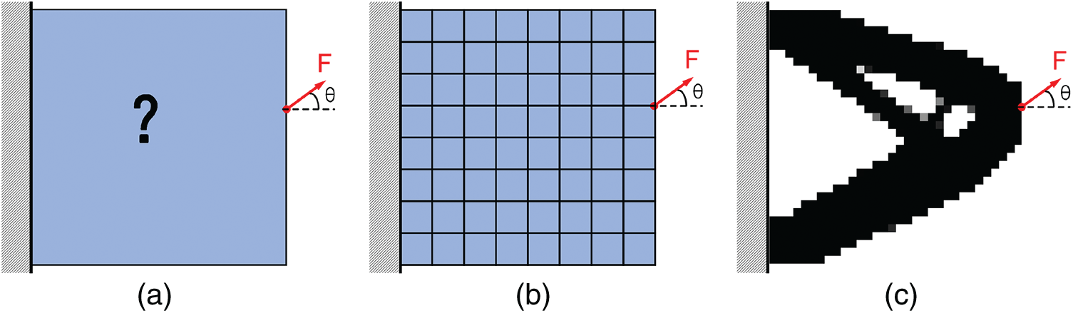
Figure 1: The illustration of 2D topology optimization using the SIMP method. (a) initial design domain, (b) finite element discretization, (c) optimized structure
The feature pyramid network is a framework to construct a feature pyramid network within CNN [18,43,44]. A lot of convolution operation is used inside FPN. Convolution operation can extract features from the given sample and is widely used in signal processing and image recognition. As shown in Fig. 2a, features are extracted using a convolutional filter. The convolutional filter progresses regularly on the input image and generates a feature image as the output. The stride represents the number of convolutional filters moving in each step. The advantage of feature pyramid networks is pyramidal feature hierarchy (Fig. 2b). Pyramid feature hierarchy produces a multi-scale feature representation, which can express features of different scales. And the semantic strength of each layer is different. The thicker outlines in Fig. 2b indicate semantically stronger features. In order to better capture different scale semantic specificities for output prediction, FPN uses a top-down way architecture with lateral connections to build high-level semantic feature maps across all scales. Fig. 3 is the architecture of the feature pyramid network for 2D topology optimization in this study, from which we can see the main components of FPN. It consists of: bottom-up pathway, top-down pathway, lateral connections, and aggregation.
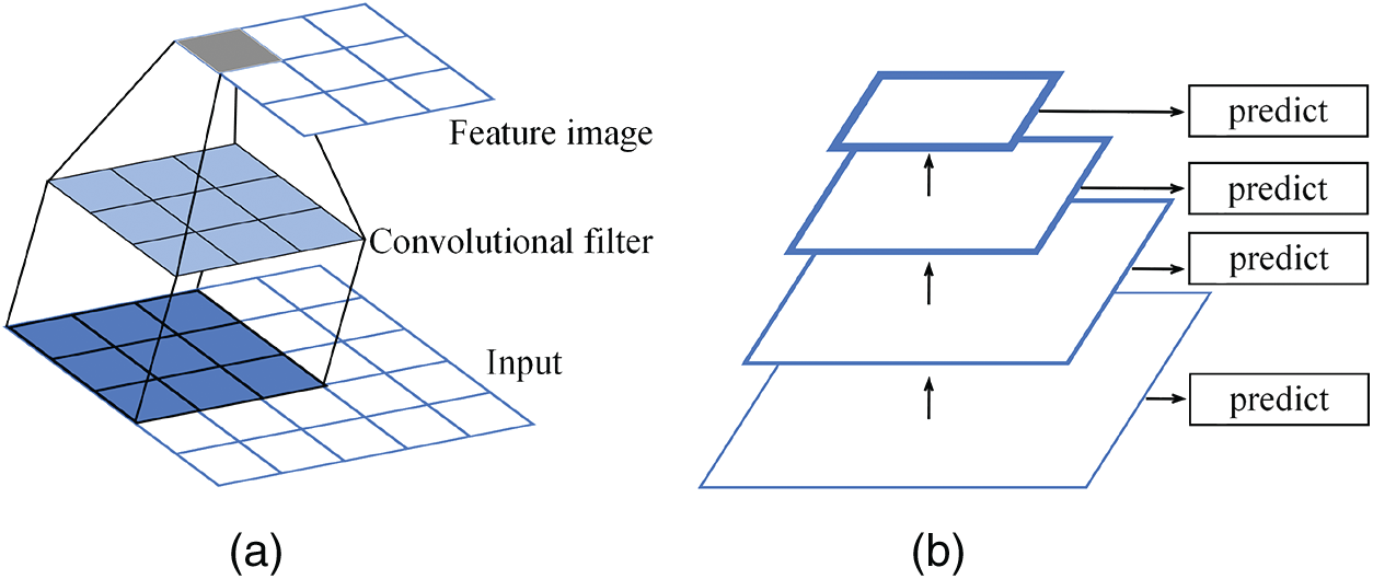
Figure 2: Schematic of the basic neural network. (a) Example of a convolutional neural network with a stride of one, (b) Pyramidal feature hierarchy and thicker outlines denote semantically stronger features
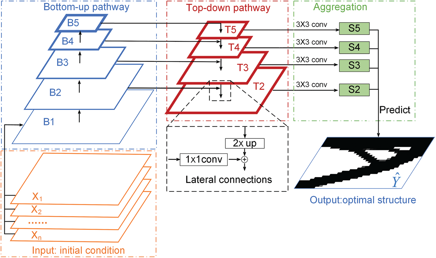
Figure 3: The overall architecture of the feature pyramid network used in our work for 2D topology optimization. The bottom-up pathway (blue) consists of five levels at different scales. The top-down pathway (red) builds semantically stronger features by upsampling spatially coarser feature images from higher pyramid levels. Lateral connections (black) connect the bottom-up pathway and the top-down pathway. The aggregation (green) coalesces feature maps of these different levels to complete the final prediction
Some deep neural networks were developed to accelerate topology optimization design before this study, including U-net [45], ResUnet [29], and others. The ResUnet has more residual learning [46] than U-net to solve the problem of vanishing gradients and improve performance further. U-net and ResUnet concatenate low-level detail information and high-level semantic information, namely skip connections, to improve segmentation accuracy. Encoder, decoder, and skip connections in U-net and ResUnet are similar to bottom-up pathway, top-down pathway, and lateral connections in FPN, respectively.
However, the reasons why FPN is used in this study are as follows. Firstly, the optimization structure of the model output will change with the difference of input boundary conditions, volume fractions, loads, and filter radius in this study. These input channels contain information with different physical multi-scale structural semantics. Aggregation (Fig. 3) represents the fusion prediction of multi-scale feature maps, which can reduce the error than summation-based architectures [1]. This advantage can help the output of optimized structures to be more accurate and acquire prediction models with higher precision. Aggregation from different levels is not utilized in U-net and ResUnet model. In addition, FPN can use ResNets [46] of different layers (18, 34, 50, 101, 152) to quickly build a suitable network model according to the complexity of different topology optimization problems. FPN has high computation and memory efficiency, which provides a practical and accurate solution for multi-scale semantic modeling. Based on the above considerations, we adopt FPN to implement the regression task.
Before conducting experimental research, we need to make full preparations, of which we prepare for two main aspects: data preparations and CNN architectures.
3.1 Data Generation and Processing
We prepare two types of datasets generated from two classic topology optimization problems, including Cantilever Beam (Fig. 1) and MBB Beam (Fig. 4). The material is linear elastic material conforming to Hooke’s law. Each dataset consists of a number of topology optimizations which include boundary conditions, loads, and volume fractions in each sample. In the process of generating Cantilever Beam data, we have made a certain comparison with the related work of Abueidda et al. [28] and Yu et al. [47]. The design domain adopts a
• Resolution:
• Volume fraction: [0.3, 0.7]
• Load position: the node selected from the set of nodes at the right-hand side of the design space
• Load direction: [0, 360
• SIMP penalty: 3
• SIMP filter radius: 1.5
Once these parameters are obtained, the 88 lines [48] SIMP method is used to generate optimized structures with five dataset scales: 6000, 12000, 18000, 24000, and 30000. Different datasets are used to test the learning ability of the proposed model. These datasets will be saved to text files, including all required information for later experiments. In order to facilitate the input and output of the neural network with datasets, we adopted a similar composition method referred by [28] to generate the dataset with five channels and a label. The number of elements in the design domain is
We also chose the classic MBB Beam topology optimization model. In this model, the finite element mesh discrete linear elastic structure of
• Resolution:
• Volume fraction: [0.3, 0.7]
• Load region: x = [1, 33], y = [1, 33]
• Load direction: 270
• SIMP penalty: 3
• SIMP filter radius: [1.5, 4.5]
Since the size of the design domain is different, the parameters will be changed accordingly. As shown in Fig. 4, the design space becomes a rectangle. The angle of the applied force becomes a constant 270 degrees. The loading location changed from a line on the right to an area on the left. The filter radius changed from fixed
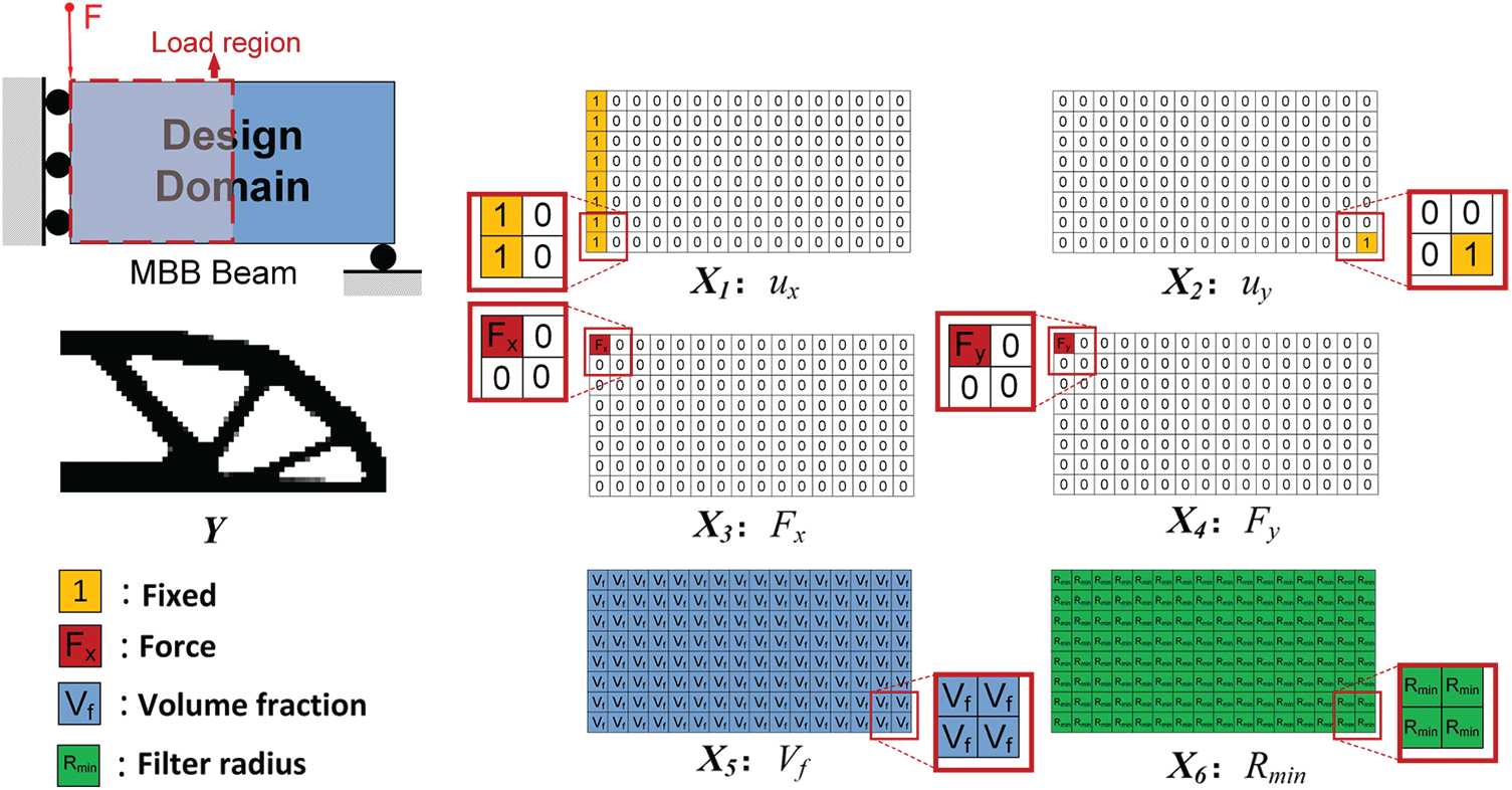
Figure 4: Discretization of different channels on the MBB Beam
The training set is used to train the model and find the parameters of the neural network model. The validation set is used to evaluate the convergence performance of the model training. The test set is used to provide a final evaluation after the model training process. In order to train the FPN model effectively and evaluate the model performance accurately, the ratio of the training set, the validation set, and the test set is 8:1:1 in each dataset, respectively.
3.2 The Architecture of the Neural Network
According to the characteristics of this study, the input and output channels of the same design problem are basically fixed. In this section, we will choose one of the two design problems arbitrarily as the modeling object to describe the details of the network architecture. As shown in Fig. 5, we took the
Bottom-up pathway: The blue layer represents the bottom-up pathway in Fig. 5. This path is the process of continuous feedforward calculation of CNN structure. We adopted ResNet18 as the main framework of the neural network structure. The structure of the neural network can be changed on a small scale according to different problems. ResNet with other layers can also be used to build the framework of the neural network structure. Since the size of the input and output channels is small in this problem, The FPN using ResNet18 as the main structure can meet the requirements. In the bottom-up pathway, as shown in Fig. 3, we use five main layers.
Top-down pathway: The red layer represents the top-down pathway in Fig. 5. By building the feature pyramid network structure, the low-level features can be improved so that the features on the higher layer of the pyramid can represent the global semantic features. A top-down pathway can pass the global semantic features acquired from the high-level down to the low-level, with lateral connections to improve more accuracy. This process changes the resolution of the channel from lower to higher. This architecture uses four layers
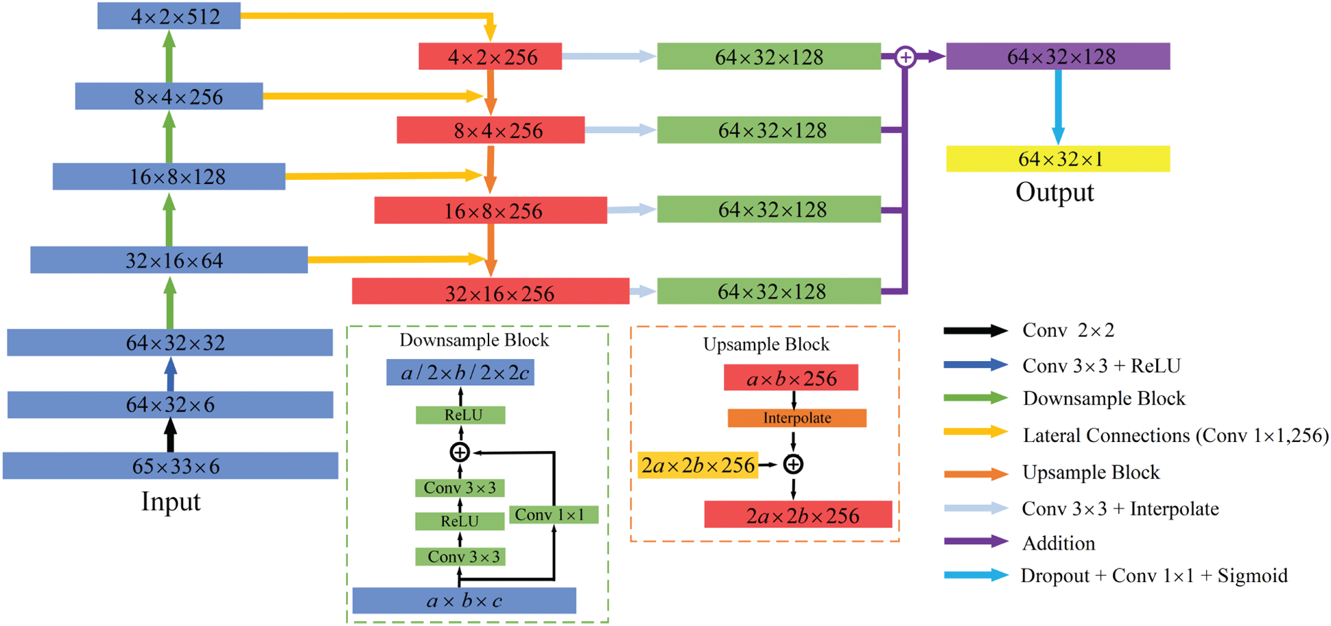
Figure 5: The architecture of the neural network for MBB Beam topology optimization datasets
Lateral connections: Fig. 5 shows that yellow arrows display the process of lateral connections. Lateral connections can be understood as that the feature map drawn through the top-down pathway is strengthened with the corresponding bottom-up feature map by element-wise addition using a
Aggregation: Each level at the top-down pathway is asked to make a prediction and the feature map is semantically strong at different levels. In order to complete the final prediction of the optimization structure, it is necessary to aggregate feature maps of these different levels. Before aggregation, the feature map set
This section will elaborate on the problems to be studied in detail from three aspects, including the topology optimization framework of deep learning with physical constraints, physical constraints, and evaluating metrics of our networks.
4.1 The Topology Optimization Framework Using Deep Learning with Physical Constraints
Due to high computational cost for complex engineering structure design or the lack of physical performance as discussed in the introduction, the main goal of our work is to obtain a prediction model that can be used to obtain the optimization structure quickly under different initial conditions, thus presenting a deep learning model with physical constraints assisted topology optimization framework. Fig. 6 illustrates the topology optimization framework using deep learning with physical constraints so as to get a predicting model. The framework consists of three main processes: data preparation, model training, and model testing.
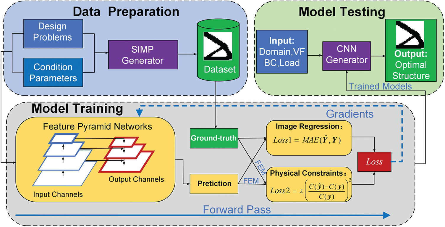
Figure 6: The illustration of the topology optimization framework of deep learning with physical constraints in the experiment
Data preparation: With given design problems and condition parameters, the SIMP method is used to generate a certain number of datasets, which can be used as training sets, validation sets, and test sets. Two different design problems and different sample scales will be generated to verify the applicability of the proposed model. It should be considered that these training samples are evenly distributed in the design space as much as possible for obtaining a more accurate predicting model.
Model training: The multi-channel matrix generated by condition parameters is taken as the input to the FPN. The optimized structure generated by the SIMP method serves as the label for the FPN training. On the one hand, the main part of mapping modeling is seen as an image-to-image regression task. On the other hand, by adding physical constraints to the loss function, the modeling process is also a regression task in physical meaning. Weight parameters are iteratively optimized through gradient backpropagation of the loss function in the network. In this way, the loss function (Section 4.2) with a physical constraint makes the trained model predict the optimization structure with a better physical performance. FPN is used for the first time to learn the inherent law of topology optimization samples. In addition to ensuring the mapping accuracy of the training set, the trained model is also required to have a good generalization ability to new samples.
Model testing: When the predicting model is constructed, the accuracy and generalization ability of the model are tested by predicting the optimization structure with some new samples. The model can be used to solve the topology optimization problem quickly with a preferable physical performance. The performance of the test results is also beneficial to adjust the hyperparameters of the training model in the next stage.
There are three processes where the finite element method (FEM) solver will be needed throughout the whole experiment. First, in the process of data generation, The FEM solver is one of the components of the SIMP generator during the iteration process of topology optimization. Secondly, the FEM solver needs to be used in the calculation of loss function during model training. Finally, during model testing, the FEM solver is required to calculate the compliance (
When the loss function of model training is only based on the pixel-wise error from image perspectives, some predicted structural compliance may not meet physical requirements. Therefore, by introducing physical constraints to the loss function, the model training is an image-to-image mapping relationship with pixel-wise errors and physical meanings. The addition of physical constraints can better solve the above problem. In this way, there is one more constraint index for the model training. In this study, the mean absolute error (MAE) and the mean squared error (MSE) which are common loss functions for image-to-image regression tasks are feasible. Considering that the convergence rate of MAE is faster than that of MSE in the use of sigmoid function, the characteristic allows physical constraints to be added earlier and helps model training save time better. Therefore, MAE is used as the basis of loss function for the FPN model.
For the Loss function, Eq. (3) is constructed as above. It is the sum of Loss1 and Loss2. Loss1 means the mean absolute error and is defined as follows:
N represents the total number of meshes in the design domain.
In order to evaluate the performance of our model reasonably in this study, we adopt REC, REV, and ACC as evaluation metrics, of which REC is the most indicative metric. The three evaluation metrics are explained as follows:
1. REC is the relative error between the compliance of the prediction structure
2. REV is the volume relative error between the prediction structure
3. Pixel-wise accuracy (ACC) is a vital evaluation metric in the field of image segmentation. In this study, we employ it to measure the similarity between two material distribution maps. As shown in Eq. (8), n0 represents the total number of the distribution map pixels equal to 0. n1 represents the total number of the distribution map pixels equal to 1. w11 stands for the sum of the distribution map points whose ground-truth value and predicted value are 1. w00 stands for the sum of the distribution map points whose ground-truth value and predicted value are 0.
In this section, we firstly choose two classical topology optimization problems as research objects to validate the feasibility and efficacy of model training with physical constraints. Then, we study the relationship between the training dataset scale and the prediction performance. Finally, we discuss the influence of weight factors on prediction accuracy. In each subsection, we will demonstrate, explain and discuss the experimental results. The research in this paper is based on PyTorch 1.4 and the model training uses a single NVIDIA TITAN RTX card equipped with 32 GB of device memory. The optimizer is Adam [49].
5.1 Performance of Model Training with Physical Constraints
In this section, in order to illustrate the effectiveness of the proposed method, we define two models: Model1 (Loss = Loss1) and Model2 (Loss = Loss1+Loss2). The loss function of Model1 is MAE. The loss function of Model2 has more physical constraints than Model1. According to some experimental results obtained in the early stage, for better training models, we set the hyperparameters to the three cases: the number of epochs of 180, the learning rate of 0.01, and the batch size of 64 for each model. The dataset scale for two classical topology optimization problems is 6000. We chose the Cantilever Beam from two topology optimization problems as a representative to illustrate the process and performance of adding physical constraints to the loss function. The main neural network architecture is similar to Fig. 5, of which the input size is
Firstly, we study the training effect of Model1. The loss history curves during the training and validation are shown in Figs. 7a and 7b. It can be seen from Fig. 7a that the loss function converges stably in both the training set and the validation set. Moreover, the difference between the validation loss and training loss is small. The FPN model reaches a relatively stable convergence in the first 100 epochs, and the model converges to the minimum value in the last 80 epochs. As shown in Fig. 7b, Loss2 is calculated by the ground-truth and the output structure obtained during Model1 training and validation. Note that the value of Loss2 is over 10 and has large fluctuation in the beginning. As training goes on, the Loss2 curve tends to converge stably. The reason for the Loss2 curve with large fluctuation is that when the training has not been completed the output structure has not been well optimized, resulting in large structural compliance. If compliance constraint is added to Loss at the beginning of training, the convergence of training will be affected. Therefore, we adopt the strategy that compliance constraint is added to Loss when model training (Loss = Loss1) converges to a relatively stable state and Loss2 is the same order of magnitude as Loss1. This operation prevents a large value of Loss2 from making the failure of the model convergence at the beginning of the model training.
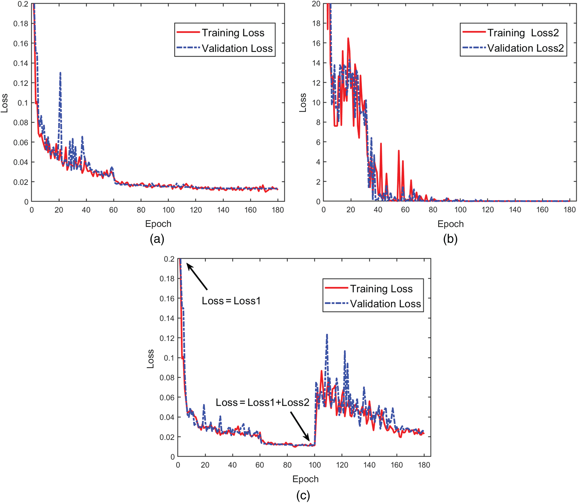
Figure 7: The convergence history of Model1 and Model2 with compliance constraints. (a) Training loss and validation loss (Loss = Loss1) on Model1, (b) Training Loss2 and validation Loss2 calculated during Model1 training, and (c) Training loss and validation loss on Model2 (the first 100 epochs: Loss = Loss1, and the last 80 epochs: Loss = Loss1+Loss2)
Fig. 7c illustrates the loss function of Model2 in the training set and validation set. At the training of 100 epochs, we add Loss2 to the loss function to continue training. Then, the training process is stopped when the validation loss reaches the minimum value after 180 epochs. From the history of the Loss curves, the value of Loss increases suddenly and then decreases gradually to stable. The reason for the curve change is that the model converges in physical meaning after adding compliance constraints to the training.
After Loss2 is added to the loss function, the finite element analysis is needed for the calculation of compliance, and each iteration takes a certain amount of time. Therefore, the model does not incorporate physical constraints at the beginning of model training, which can save a lot of time and improve training efficiency. Fig. 8 shows the training time of different design problems with 6000 samples. During the training process on the Cantilever Beam, the training time of Model1 is 3.5 h, and the training time of Model2 is 12.7 h. It can be seen that the addition of Loss2 requires finite element calculation, which increases the training time by several times.
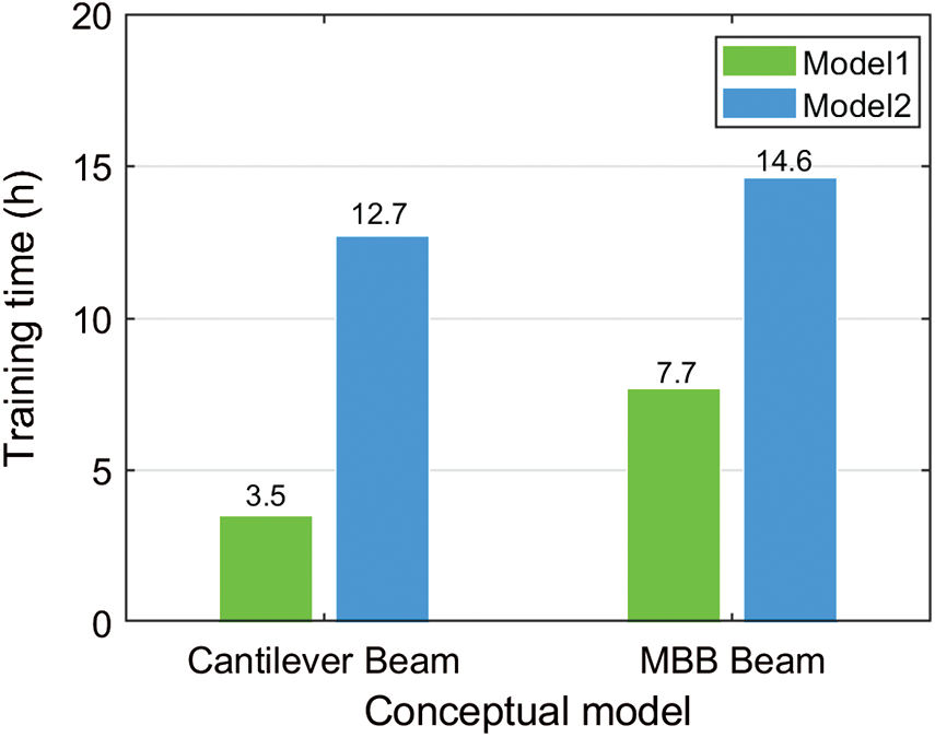
Figure 8: Comparison of training time between Model1 and Model2
Fig. 9 shows that the average value of each metric (REC, REV, ACC) is calculated from the ground-truth and the optimized structure predicted by Model1 and Model2 in the validation set. As can be seen from Figs. 9a and 9b, REC of Model1 gradually converges to 0.0275. REC of Model2 has a slight fluctuation and finally tends to converge to 0.0153 after 100 epochs of training. The history of REV in both Model1 and Model2 is stable, and the REV is finally obtained as 0.0125 and 0.0083, respectively. The experimental results show that REC and REV are both getting smaller after adding compliance constraints. what is clearly presented in Fig. 9c is that the history of ACC obtained by Model1 and Model2 converges stably and finally converges to 0.9856 and 0.9881, respectively. ACC of the two models is basically the same, indicating that the pixel-wise accuracy of prediction will be improved slightly after adding compliance constraints to the model. By comparing the above results, it can be concluded that the model with compliance constraints has better physical performance.
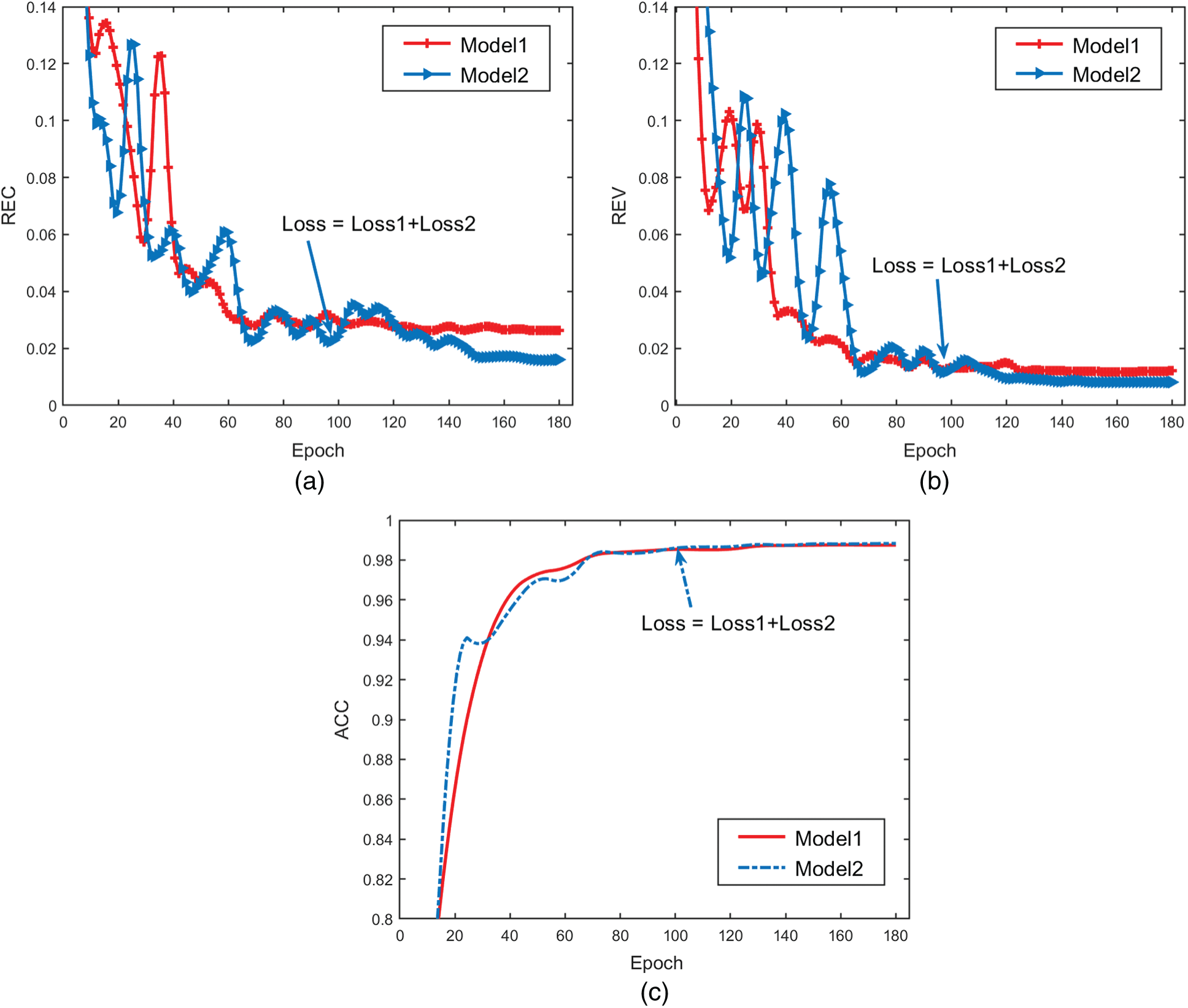
Figure 9: Metrics comparison of using different Model in the validation set. (a) REC (b) REV (c) ACC
In Fig. 10, we show some ground-truth and predicting structures, of which metrics listed on both sides. After the training process is completed, in order to better retrieve the binary nature of the solution in the test phase, element density values greater than 0.5 are set as 1, and element density values less than 0.5 are set as 0. In Section (a) of Fig. 10, It can be seen that the most optimized structure predicted by Model2 is better than the optimized structure predicted by Model1 in terms of REC, REV, and ACC. The red circle emphasizes the part of prediction structures in Fig. 10, which is a different part relative to the ground-truth or is structure disconnections. Yu et al. [47] proposed the model which provided some structural disconnections in some cases. In our study, the issue of structural disconnections is still present in Model1. However, the problem is effectively reduced in Model2, although 6000 samples are used by Model2. We use the same sample scales, steps, and methods to study the MBB Beam. The results obtained from the experiment are shown in Section (a) of Fig. 10. By comparing the results, it is found that the test performance on the MBB Beam is similar to that on the Cantilever Beam. Therefore, it can be concluded that model training with compliance constraints can improve the physical performance of the prediction results. The proposed method has high prediction accuracy and physical performance in both problems, indicating that the proposed model has good applicability.
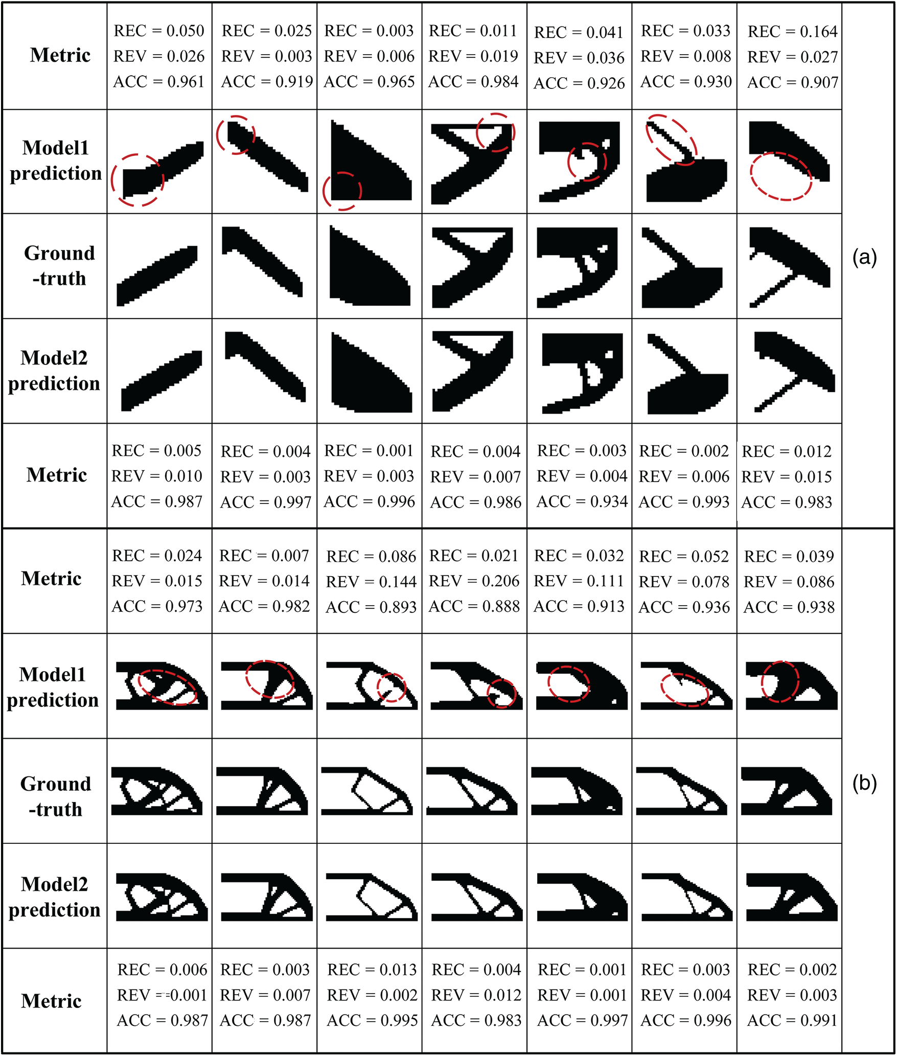
Figure 10: Comparison of prediction between Model1 without compliance constraints and Model2 with compliance constraints. (a) Cantilever Beam, (b) MBB Beam
5.2 The Relationship between the Training Dataset Scale and the Prediction Performance
In order to discuss the relationship between the training dataset scale and the prediction performance in this section, Sample sets with different data scales (6000, 12000, 18000, 24000, 30000) generated in Section 3.1 are used for training models where two classical topology optimization problems are selected: Cantilever Beam and MBB Beam. Each Cantilever Beam sample consists of five channels and a sample label. And each MBB Beam sample consists of six channels and a sample label. These experiments use samples with different channel numbers to test the flexible learning ability of the model and the adaptability of the network for various boundary constraints.
The results of Model1 are summarized in Tab. 1. As shown in the green bar chart in Fig. 11, for two design problems, the changing trend of metrics can be clearly obtained in the test set. The number of MBB Beam samples increases proportionally from 6000 to 30000. REC gradually fells from 0.0163 to 0.0071. REV decreases from 0.0078 to 0.0044. ACC increases slowly from 0.9855 to 0.9912. Similarly, the sample scales of Cantilever Beam grow from 6000 to 30000. REC gradually fells from 0.0275 to 0.0145. REV decreases from 0.0125 to 0.059. ACC increases slowly from 0.9856 to 0.9902. From the test results of two design problems, the prediction accuracy of models is improved in general with increasing sample scales. It indicates that the larger number of samples is given, the better prediction accuracy of models can be obtained. This performance naturally conforms to the conclusion that the CNN model trained by more training data has better performance while keeping the other parameters constant.

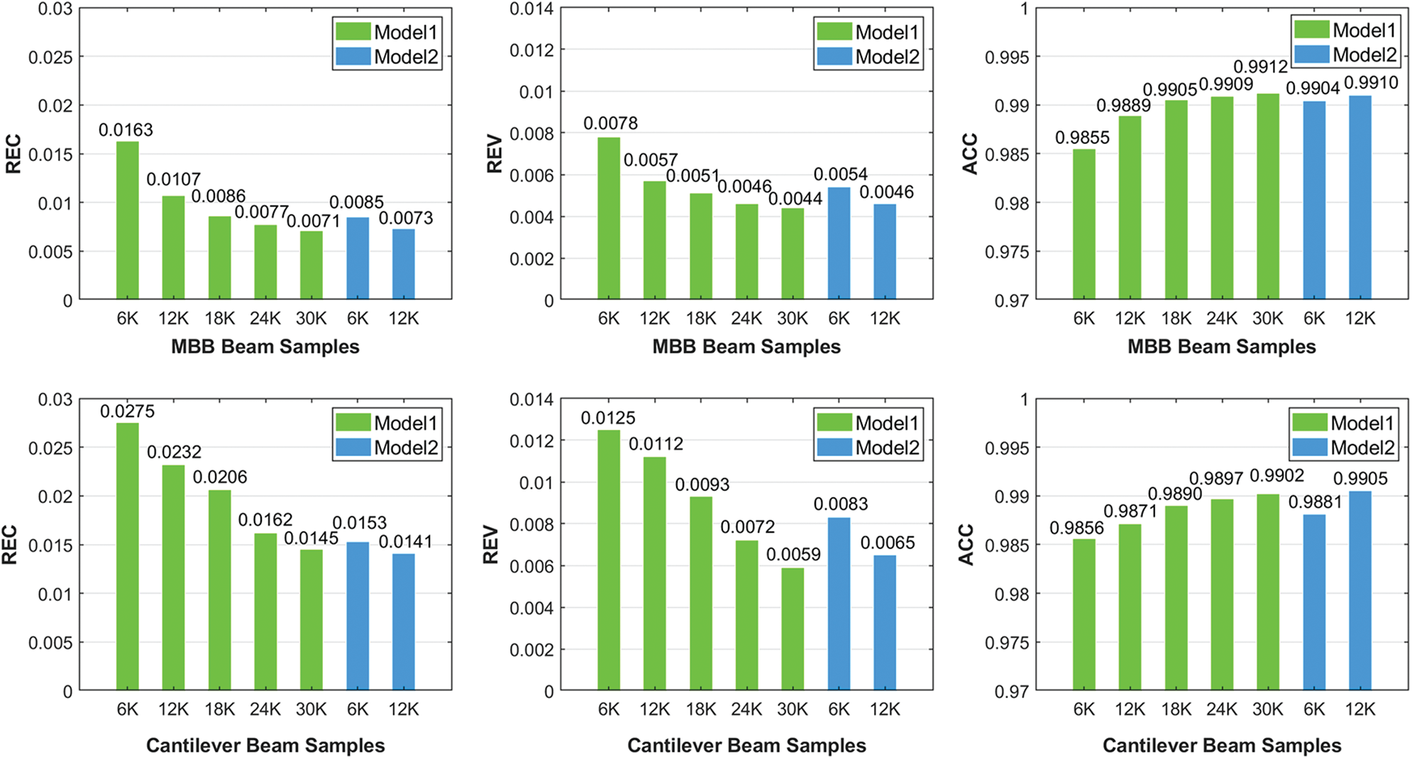
Figure 11: Performance on the MBB Beam and Cantilever Beam using different sample scales for different models. (a) REC (b) REV (c) ACC
The results of Model2 are summarized in Tab. 2 and are visualized as the blue bar chart in Fig. 11. In Tab. 2, we can observe that Model2 which uses the larger sample scale on different design problems will get better prediction accuracy. The same conclusion is shown in Tab. 1. REC, REV, and ACC of the Model2 trained with 6000 samples of Cantilever Beam are respectively 0.0153, 0.0083, and 0.9881. Compared with Model1, it can be apparently observed that the prediction performance of Model2 has seen a big improvement by 44.36%, 33.60%, and 0.2536% in terms of REC, REV, and ACC, respectively. Similarly, REC, REV, and ACC of the Model2 trained with 6000 samples of MBB Beam are respectively 0.0085, 0.0054, and 0.9904, with a big improvement by 47.85%, 30.76%, and 0.4972% than Model1. The general trend is also seen in 12000 samples. Hence it can be concluded that the inclusion of compliance constraints improves the prediction accuracy of the trained model. In addition, this phenomenon is reflected in two different design problems, which indicates that the model has good applicability for different design problems.

Another interesting observation is that the metric performance of Model2 with 6000 samples has reached that of Model1 with 24000 samples on Cantilever Beam. Similarly, the metric performance of Model2 with 6000 samples is close to that of Model1 with 18000 samples on Cantilever Beam. The explanation is, models trained with compliance constraints also converges in physical meaning leading to model training more effective. Therefore, we can draw a conclusion that the predicted performance of the Model2 trained by small samples with compliance constraints can reach that of the Model1 trained by large samples without compliance constraints.
As shown in Section (a) of Fig. 12, the comparison between the ground-truth and the optimization structure predicted by the Model1 trained by 18000 samples and the Model2 trained by 6000 samples on the MBB Beam. Section (b) of Fig. 12 shows some similar results on the Cantilever Beam, of which Model1 is obtained by 24000 samples and Model2 is obtained by 6000 samples. It can be found that the structures obtained from the proposed model almost coincide with the ground-truth results. By comparing metrics of the structures, the predicting performance of Model2 trained on a small number of samples is the same as the predicting performance of Model1 trained on a large number of samples. It can be verified that model training with physical constraints is more effective. Models with physical constraints require a smaller number of samples to achieve better predicting performance. For different design problems, the performance of the model training with physical constraints has a slight change.
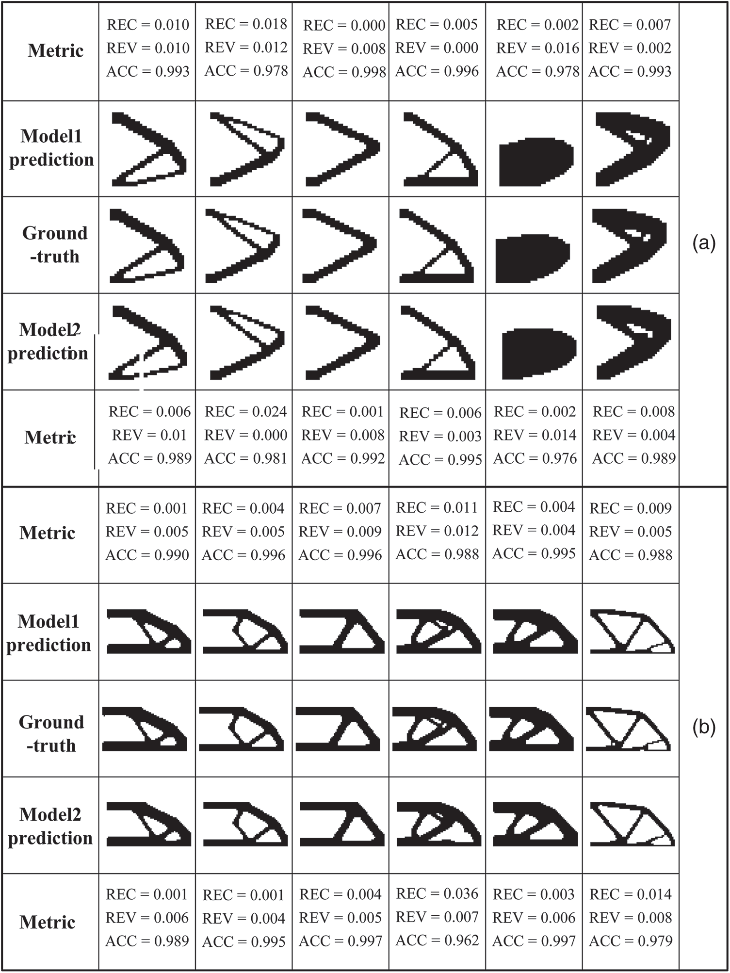
Figure 12: Comparison of prediction results between Model1 with a larger number of samples and Model2 with a smaller number of samples. (a) Model1 using 18000 samples and Model2 using 6000 samples on the Cantilever Beam, (b) Model1 using 24000 samples and Model2 using 6000 samples on the MBB Beam
5.3 The Relationship between the Weight Factor and the Prediction Performance
Although model training with compliance constraints is proven to be effective, it is worth investigating the effect of loss function with different proportions constraints. Thus, a Cantilever Beam dataset with the number of 6000 is selected to test the effect of different weight factors in this section. The goal is to find a better weight factor that helps to get a model with a a better generalization ability. The investigated loss function is expressed as Eq. (3).
We designed different proportions constraints
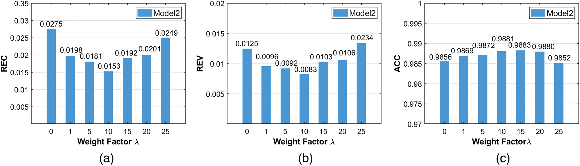
Figure 13: The performance of trained Model2 with different weight factor (
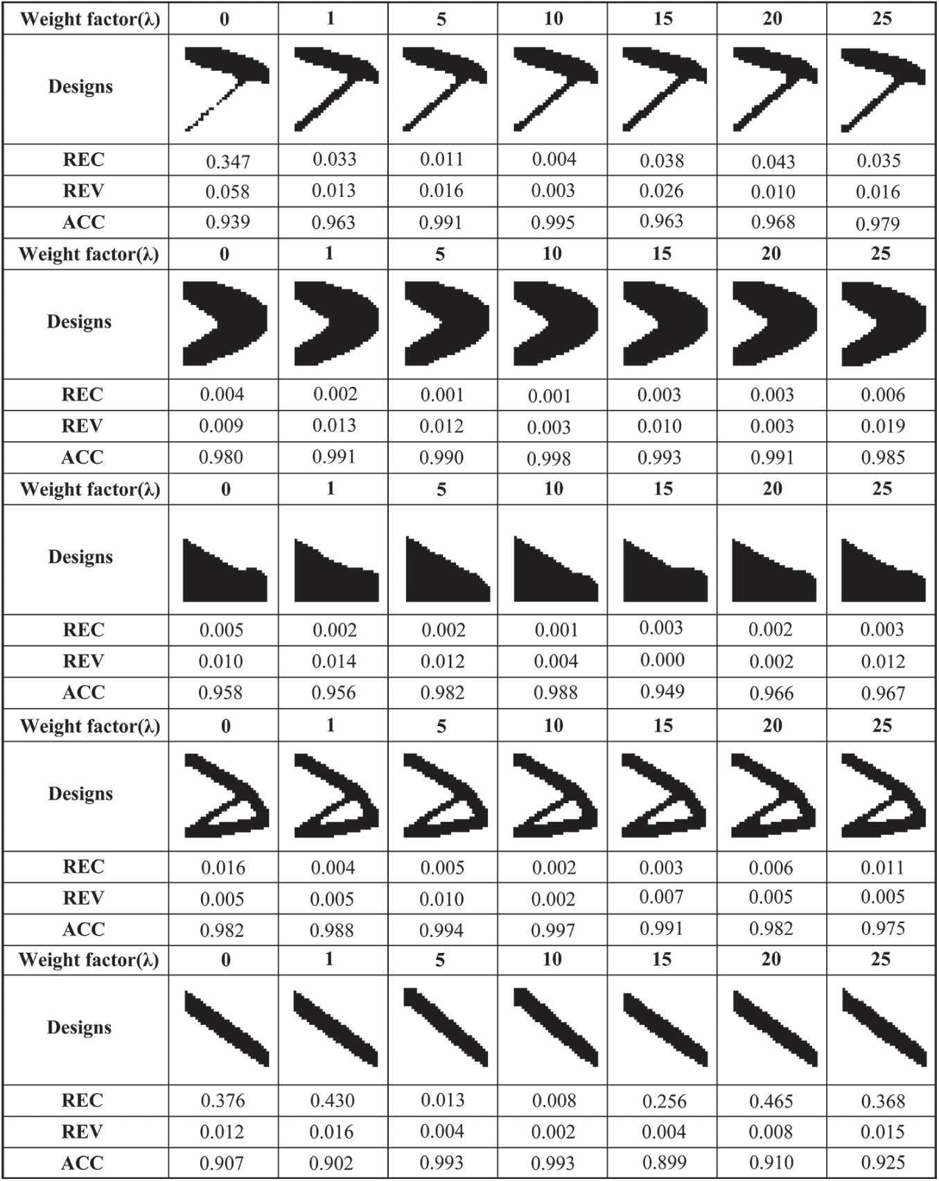
Figure 14: Optimized cantilever designs corresponding to different weight factors (
In this paper, we use the feature pyramid network for the first time as a mapping model for topology optimization design. At the same time, physical constraints are firstly added to CNN models to accelerate the solution of topology optimization, of which we adopt the proper strategy that physical constraints are reasonably added to the loss function to achieve a balance between the training cost and the training effect. According to the obtained results, it is concluded that the model training with physical constraints is able to reduce structural disconnection cases and ensure high accuracy results with a good physical performance. Besides, two classical topology optimization problems with different sample scales are selected to conduct experiments to demonstrate the feasibility of adding physical constraints. A general trend can be obtained that larger-scale data for model training can acquire better model prediction performance despite some metric fluctuation on the test set.
Compared with the traditional topology optimization method, the proposed method can quickly predict the optimization structure without any iterations. Compared with most methods of neural networks accelerating topology optimization, this method achieves a prediction model with better physical performance. The major contribution of the paper is the capability of the proposed approach, which can significantly improve the physical performance of the prediction structure. And the method requires a small number of samples to obtain the high-precision prediction model. Furthermore, FPN has the advantage that the input form can be changed flexibly according to different design problems.
In future work, we will extend the current method to solve 3D topology optimization problems. The weight factor of physical constraints will be studied further by adopting different tuning methods in the reasonable design. In addition, it is also an important direction to train high-precision models with fewer samples. The proposed method is an innovative and valuable attempt to use deep learning technology to guide topology optimization in the rapid preliminary design and accelerate the application of topology optimization technology in intelligent design.
Funding Statement: This work was supported in part by National Natural Science Foundation of China under Grant Nos. 11725211, 52005505, and 62001502, and Post-graduate Scientific Research Innovation Project of Hunan Province under Grant No. CX20200023.
Conflicts of Interest: The authors declare that they have no conflicts of interest to report regarding the present study.
1. Honari, S., Yosinski, J., Vincent, P., Pal, C. (2016). Recombinator networks: Learning coarse-to-fine feature aggregation. 2016 IEEE Conference on Computer Vision and Pattern Recognition. Las Vegas, USA. [Google Scholar]
2. Bendsoe, M. P. (1989). Optimal shape design as a material distribution problem. Structural Optimization, 1(4), 193–202. DOI 10.1007/BF01650949. [Google Scholar] [CrossRef]
3. Zhou, M., Rozvany, G. (1991). The COC algorithm, part II: Topological, geometrical and generalized shape optimization. Computer Methods in Applied Mechanics and Engineering, 89(1), 309–336. DOI 10.1016/0045-7825(91)90046-9. [Google Scholar] [CrossRef]
4. Rozvany, G. I. N., Zhou, M., Birker, T. (1992). Generalized shape optimization without homogenization. Structural Optimization, 4(3), 250–252. DOI 10.1007/BF01742754. [Google Scholar] [CrossRef]
5. Chen, Z., Long, K., Wen, P., Nouman, S. (2020). Fatigue-resistance topology optimization of continuum structure by penalizing the cumulative fatigue damage. Advances in Engineering Software, 150(2), 102924. DOI 10.1016/j.advengsoft.2020.102924. [Google Scholar] [CrossRef]
6. Xie, Y. M., Steven, G. P. (1993). A simple evolutionary procedure for structural optimization. Computers Structures, 49(5), 885–896. DOI 10.1016/0045-7949(93)90035-C. [Google Scholar] [CrossRef]
7. Huang, X. H., Xie, Y. M. (2006). Bidirectional evolutionary topology optimization for structures with geometrical and material nonlinearities. AIAA Journal, 45(1), 308–313. DOI 10.2514/1.25046. [Google Scholar] [CrossRef]
8. Munk, D. J., Vio, G. A., Steven, G. P. (2015). Topology and shape optimization methods using evolutionary algorithms: A review. Structural and Multidisciplinary Optimization, 52(3), 613–631. DOI 10.1007/s00158-015-1261-9. [Google Scholar] [CrossRef]
9. Zhang, Z., Zhao, Y., Du, B., Chen, X., Yao, W. (2020). Topology optimization of hyperelastic structures using a modified evolutionary topology optimization method. Structural and Multidisciplinary Optimization, 62(6), 3071–3088. DOI 10.1007/s00158-020-02654-9. [Google Scholar] [CrossRef]
10. Wang, M. Y., Wang, X., Guo, D. (2003). A level set method for structural topology optimization. Computer Methods in Applied Mechanics and Engineering, 192(1–2), 227–246. DOI 10.1016/S0045-7825(02)00559-5. [Google Scholar] [CrossRef]
11. Allaire, G., Jouve, F., Toader, A. M. (2004). Structural optimization using sensitivity analysis and a level-set method. Journal of Computational Physics, 194(1), 363–393. DOI 10.1016/j.jcp.2003.09.032. [Google Scholar] [CrossRef]
12. Guo, X., Zhang, W., Zhong, W. (2014). Doing topology optimization explicitly and geometrically–-A new moving morphable components based framework. Journal of Applied Mechanics, 81(8), 81009. DOI 10.1115/1.4027609. [Google Scholar] [CrossRef]
13. Du, B., Yao, W., Zhao, Y., Chen, X. (2019). A moving morphable voids approach for topology optimization with closed b-splines. Journal of Mechanical Design, 141(8), 81401. DOI 10.1115/1.4043369. [Google Scholar] [CrossRef]
14. Du, B., Zhao, Y., Yao, W., Wang, X., Huo, S. (2020). Multiresolution isogeometric topology optimisation using moving morphable voids. Computer Modeling in Engineering & Sciences, 122(3), 1119–1140. DOI 10.32604/cmes.2020.08859. [Google Scholar] [CrossRef]
15. Eschenauer, H. A., Kobelev, V. V., Schumacher, A. (1994). Bubble method for topology and shape optimization of structures. Structural and Multidisciplinary Optimization, 8(1), 42–51. DOI 10.1007/BF01742933. [Google Scholar] [CrossRef]
16. Cai, S., Zhang, W., Gao, T., Zhao, J. (2019). Adaptive bubble method using fixed mesh and topological derivative for structural topology optimization. Lixue Xuebao/Chinese Journal of Theoretical and Applied Mechanics, 51(4), 1235–1244. DOI 10.6052/0459-1879-18-455. [Google Scholar] [CrossRef]
17. Zhou, Y., Zhang, W., Zhu, J., Xu, Z. (2016). Feature-driven topology optimization method with signed distance function. Computer Methods in Applied Mechanics and Engineering, 310, 1–32. DOI 10.1016/j.cma.2016.06.027. [Google Scholar] [CrossRef]
18. Lecun, Y., Bottou, L., Bengio, Y., Haffner, P. (1998). Gradient-based learning applied to document recognition. Proceedings of the IEEE, 86(11), 2278–2324. DOI 10.1109/5.726791. [Google Scholar] [CrossRef]
19. Chen, X., Chen, X., Zhou, W., Zhang, J., Yao, W. (2020). The heat source layout optimization using deep learning surrogate modeling. Structural and Multidisciplinary Optimization, (62), 3127–3148. DOI 10.1007/s00158-020-02659-4. [Google Scholar] [CrossRef]
20. Singh, A. P., Medida, S., Duraisamy, K. (2017). Machine-learning-augmented predictive modeling of turbulent separated flows over airfoils. AIAA Journal, 55(7), 2215–2227. DOI 10.2514/1.J055595. [Google Scholar] [CrossRef]
21. Lee, S., Ha, J., Zokhirova, M., Moon, H., Lee, J. (2018). Background information of deep learning for structural engineering. Archives of Computational Methods in Engineering, 25(1), 121–129. DOI 10.1007/s11831-017-9237-0. [Google Scholar] [CrossRef]
22. Sosnovik, I., Oseledets, I. (2017). Neural networks for topology optimization. Russian Journal of Numerical Analysis and Mathematical Modelling, 34(4), 1–13. DOI 10.1515/mam-2019-0018. [Google Scholar] [CrossRef]
23. Zhang, Y., Peng, B., Zhou, X., Xiang, C., Wang, D. (2019). A deep convolutional neural network for topology optimization with strong generalization ability. arXiv:1901.07761. [Google Scholar]
24. Zhou, Y., Zhan, H., Zhang, W., Zhu, J., Bai, J. et al. (2020). A new data-driven topology optimization framework for structural optimization. Computers and Structures, 239, 106310. DOI 10.1016/j.compstruc.2020.106310. [Google Scholar] [CrossRef]
25. Banga, S., Gehani, H., Bhilare, S., Patel, S., Kara, L. (2018). 3D topology optimization using convolutional neural networks. arXiv:1808.07440. [Google Scholar]
26. Wang, C., Yao, S., Wang, Z., Hu, J. (2020). Deep super-resolution neural network for structural topology optimization. Engineering Optimization, 5(20), 1–14. DOI 10.1080/0305215X.2020.1849171. [Google Scholar] [CrossRef]
27. Lei, X., Liu, C., Du, Z., Zhang, W., Guo, X. (2018). Machine learning driven real time topology optimization under moving morphable component (MMC)-based framework. Journal of Applied Mechanics, 86(1), 011004. DOI 10.1115/1.4041319. [Google Scholar] [CrossRef]
28. Abueidda, D. W., Koric, S., Sobh, N. A. (2020). Topology optimization of 2D structures with nonlinearities using deep learning. Computers & Structures, 237, 106283. DOI 10.1016/j.compstruc.2020.106283. [Google Scholar] [CrossRef]
29. Zhang, Z., Liu, Q., Wang, Y. (2017). Road extraction by deep residual u-net. IEEE Geoscience and Remote Sensing Letters, 15(5), 749–753. DOI 10.1109/LGRS.2018.2802944. [Google Scholar] [CrossRef]
30. Rawat, S., Shen, M. H. (2019). Application of adversarial networks for 3D structural topology optimization. WCX SAE World Congress Experience. Detroit, Michigan. [Google Scholar]
31. Goodfellow, I., Pouget-Abadie, J., Mirza, M., Xu, B., Warde-Farley, D. et al. (2014). Generative adversarial nets. Advances in Neural Information Processing Systems, 27, 2672–2680. DOI 10.5555/2969033.2969125. [Google Scholar] [CrossRef]
32. Nie, Z., Lin, T., Jiang, H., Kara, L. B. (2021). Topologygan: Topology optimization using generative adversarial networks based on physical fields over the initial domain. Journal of Mechanical Design, 143(3), 1–13. DOI 10.1115/1.4049533. [Google Scholar] [CrossRef]
33. Nakamura, K., Suzuki, Y. (2020). Deep learning-based topological optimization for representing a user-specified design area. arXiv:2004.05461. [Google Scholar]
34. Ates, G. C., Gorguluarslan, R. M. (2021). Two-stage convolutional encoder-decoder network to improve the performance and reliability of deep learning models for topology optimization. Structural and Multidisciplinary Optimization, 63(4), 1927–1950. DOI 10.1007/s00158-020-02788-w. [Google Scholar] [CrossRef]
35. Sharma, R., Farimani, A. B., Gomes, J., Eastman, P., Pande, V. (2018). Weakly-supervised deep learning of heat transport via physics informed loss. arXiv:1807.11374. [Google Scholar]
36. Ma, H., Hu, X., Zhang, Y., Thuerey, N., Haidn, O. J. (2020). A combined data-driven and physics-driven method for steady heat conduction prediction using deep convolutional neural networks. arXiv: 2005.08119. [Google Scholar]
37. Sun, L., Gao, H., Pan, S., Wang, J. X. (2020). Surrogate modeling for fluid flows based on physics-constrained deep learning without simulation data. Computer Methods in Applied Mechanics and Engineering, 361(4), 112732. DOI 10.1016/j.cma.2019.112732. [Google Scholar] [CrossRef]
38. Lin, T. Y., Dollar, P., Girshick, R., He, K., Hariharan, B. et al. (2017). Feature pyramid networks for object detection. 2017 IEEE Conference on Computer Vision and Pattern Recognition, pp. 2117–2125. IEEE. [Google Scholar]
39. Sigmund, O., Maute, K. (2013). Topology optimization approaches. Structural and Multidisciplinary Optimization, 48(6), 1031–1055. DOI 10.1007/s00158-013-0978-6. [Google Scholar] [CrossRef]
40. Sigmund, O. (2001). A 99 line topology optimization code written in Matlab. Structural and Multidisciplinary Optimization, 21(2), 120–127. DOI 10.1007/s001580050176. [Google Scholar] [CrossRef]
41. Ambrosio, L., Buttazzo, G. (1993). An optimal design problem with perimeter penalization. Calculus of Variations and Partial Differential Equations, 1(1), 55–69. DOI 10.1007/BF02163264. [Google Scholar] [CrossRef]
42. Petersson, J. (1999). Some convergence results in perimeter-controlled topology optimization. Computer Methods in Applied Mechanics and Engineering, 171(1–2), 123–140. DOI 10.1016/S0045-7825(98)00248-5. [Google Scholar] [CrossRef]
43. Krizhevsky, A., Sutskever, I., Hinton, G. E. (2017). ImageNet classification with deep convolutional neural networks. Communications of the ACM, 60(6), 84–90. DOI 10.1145/3065386. [Google Scholar] [CrossRef]
44. Simonyan, K., Zisserman, A. (2014). Very deep convolutional networks for large-scale image recognition. Cornell University. arXiv:1409.1556. [Google Scholar]
45. Ronneberger, O., Fischer, P., Brox, T. (2015). U-net: Convolutional networks for biomedical image segmentation. International Conference on Medical Image Computing and Computer–-Assisted Intervention. Munich, Germany. [Google Scholar]
46. He, K., Zhang, X., Ren, S., Sun, J. (2016). Deep residual learning for image recognition. 2016 IEEE Conference on Computer Vision and Pattern Recognition, pp. 770–778. Las Vegas. [Google Scholar]
47. Yu, Y., Hur, T., Jung, J. (2019). Deep learning for determining a near-optimal topological design without any iteration. Structural and Multidisciplinary Optimization, 59(3), 787–799. DOI 10.1007/s00158-018-2101-5. [Google Scholar] [CrossRef]
48. Andreassen, E., Clausen, A., Schevenels, M., Lazarov, B. S., Sigmund, O. (2011). Efficient topology optimization in MATLAB using 88 lines of code. Structural and Multidisciplinary Optimization, 43(1), 1–16. DOI 10.1007/s00158-010-0594-7. [Google Scholar] [CrossRef]
49. Kingma, D. P., Ba, J. (2014). Adam: A method for stochastic optimization. 3rd International Conference on Learning Representations. San Diego, USA. [Google Scholar]
 | This work is licensed under a Creative Commons Attribution 4.0 International License, which permits unrestricted use, distribution, and reproduction in any medium, provided the original work is properly cited. |